Division II (include assigned division number from I to X)
Simulation of Ductile Crack Growth in Cracked Pipes Using the GTN Model
Young-Ryun Oh1, Hyun-Suk Nam1, Naoki Miura2, Yun-Jae Kim3
1 Graduate Student, Mechanical Engineering, Korea University, Korea 2 Doctor, Central Research Institute of Electric Power Industry, Japan 3 Professor, Mechanical Engineering, Korea University, Korea
ABSTRACT
In this paper, the GTN model is applied to simulate ductile crack growth in through-wall cracked STPT410 carbon steel pipes and simulation results are compared with experimental data. Three issues related to practical application of the GTN model to ductile crack growth simulation in cracked pipes are addressed. The first one is how to determine the GTN parameters from test data. The second issue is how to determine values of damage parameters according to the element-size. The third one is the effect of the crack-tip mesh design on values of damage parameters. This paper explains how to determine the GTN model parameters from fracture toughness (J-R) data. The effects of the element size and crack-tip mesh design on the GTN parameters are also presented. Ductile crack growth simulation of the cracked pipe is performed using the determined GTN model and simulation results are compared with experimental data.
INTRODUCTION
Ductile failure simulation using finite element (FE) methods can be efficiently used to predict fracture behaviour of cracked piping components. Among ductile failure damage models, the Gurson-Tvergaard-Needleman (GTN) model (Gurson, 1977; Chu, 1980; Tvergaard, 1984) has been wieldy used. It
has been
extensively applied to simulate ductile fracture of small-scale experiments such as tensile and
fracture toughness te
st. Despite its popularity, one difficulty in application of the GTN model is to determine its parameters from limited mechanical test data. There may be several ways to determine the parameters but detailed procedures may depend on researchers (Rakin, 2008; Xue, 2010; Schmitt, 1997). The GTN model has been also applied to simulate ductile crack growth in cracked pipes (Xu, 2010; Ruggieri, 2011; Hojo, 2013), but simulation is typically limited to small amount of crack growth. It is partly because a small element size of 50 to 200 μm has been often used in crack growth simulation of metallic structures, which corresponds to a microstructural length scale for dimple fracture. The use of such small elements makes long stable ductile crack growth simulation computationally difficult and unstable. A simple way to solve this problem would be to increase the element size, but the damage parameters should be determined for the element size used in damage analysis. For Shatil (2000) and Acharyya (2008), the effect of the element size on damage simulation of tensile and cracked pipe tests was confirmed. Kiran (2014) investigated the relationship between the element size and the GTN parameter (one parameter related to void volume fraction) based on notch tensile test results. Although existing works have suggested that the GTN parameters are dependent on the element size, no systematic investigation on how to quantify the element-size-dependency of the GTN parameters to simulate long stable crack growth in cracked pipes.GURSON-TVERGAARD-NEEDLEMAN MODEL
*
(
)
for
for
F c
c c c F
F c
F F
f
f
f
f
f
f
f
f
f
f
f
f
f
f
−
=
+
−
< <
−
≥
(2)
where is the critical void volume fraction; is void volume fraction at final fracture; and F = 1 .
The evolution equation for f is given by
2
1
(1
)
exp(
(
) )
2
2
pl N p N kk pl N Nf
f
f
s
s
ε
ε
ε
ε
π
•−
= −
+
−
(3)where is the volume fraction of particles available for void nucleation; is the mean void nucleation strain; is the standard deviation of the distribution; is plastic hydrostatic strain rate; is the equivalent plastic strain in the matrix material; and is the equivalent plastic strain rate in the matrix material.
DETERMINATION OF THE GTN MODEL DAMAGE PARAMETERS
Summary of mechanical test results
This paper considers a series of test data performed at Central Research Institute of Electric Power Industry (CRIEPI) in Japan. The material was STPT410 carbon steel in Japanese Industrial Standard. Tensile test specimens with the 5 mm diameter and 25 mm gauge length were taken from 12B Schedule 40 pipes. Tensile test was conducted at 300 ̊C. More information can be found in Ref. (Miura, 2007). Fracture toughness test was conducted using three 1/2T C(T) specimens. The side-groove of 11 % of the total thickness was machined in both sides.
Determination of the GTN parameters using by mesh type I
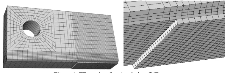
To determine the parameters in the GTN model for STPT 410, FE damage analysis is performed to simulate the C(T) test. Figure 1 shows the FE model. A quarter model was used considering symmetry conditions. Eight-node brick elements with reduced integrations (C3D8R within ABAQUS) were uniformly spaced in the crack propagation region. The minimum element size Le in the crack propagation
Figure 1. FE meshes for simulating C(T) test
In simulation, the parameters in the GTN model should be assumed a priori. The first trial is to choose one parameter for fitting (here, ) while all other parameters are fixed to assumed values. Based on the review in Section 2.2, the following values were assumed; = 1.44, = 0.94, = 0.10 and = 0.20. The void nucleation term is neglected and thus = 0 is assumed. Note that the values of = 0.3 and = 0.1 were assigned to avoid numerical floating error (see Eq. (3)). Numerical computations are performed using the ABAQUS explicit with the embedded porous plasticity model.
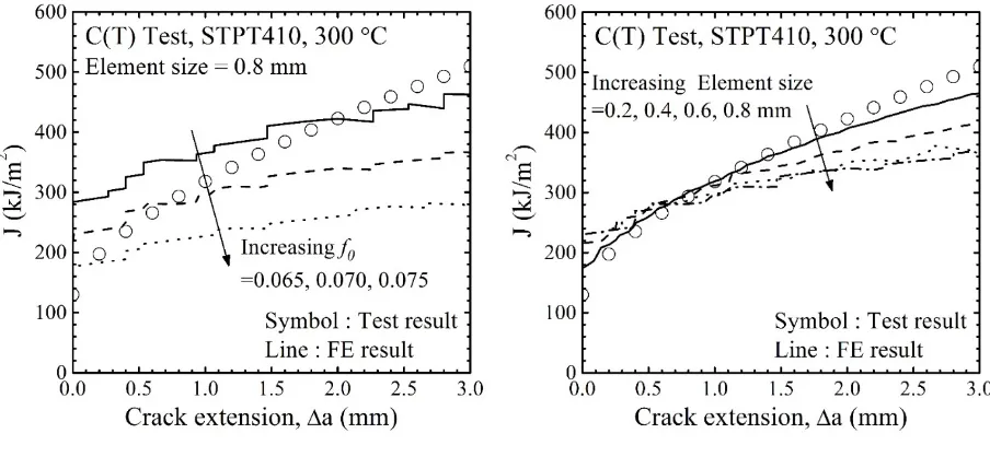
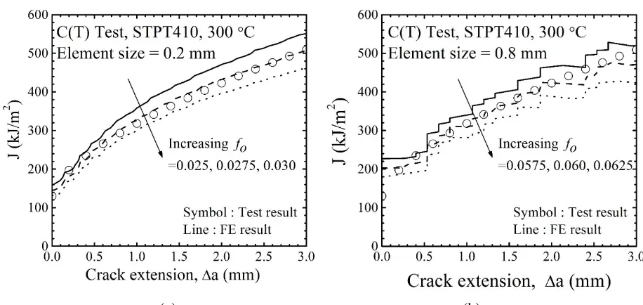
We decided to choose two parameters, and , as calibration variables. The values of was varied in the range of 0.03 to 0.05, whereas that of in the range of 0.1 to 0.3. Through iterative process, values of = 0.0315 and = 0.1 were chosen. Corresponding simulation results are compared with experimental data in Figure 2(a) and the final set of the GTN model parameters is summarized in Tables 1 and 2.
(a) (b)
Figure 2. (a) Comparison of FE simulation results (Le = 0.2 mm) with experimental J-R data, and (b) the
effect of the element size Le on FE simulation results.
To investigate the effect of the element size on the GTN model parameters, FE damage analyses using different element sizes (Le = 0.4, 0.6 and 0.8 mm) were performed to simulate the C(T) test. Values of the
GTN model parameters for various element size (0.4, 0.6 and 0.8 mm) are the same as those given in Table 1 and = 0.0315 found for Le = 0.2 mm was used. Simulation results are shown in Figure 2(b).
To find the GTN damage model parameters for larger element sizes, all other parameters except were fixed to the values given in Table 1. Then the value of was varied. Figure 3(a) shows the effect of on simulated J-R curves for the case of Le = 0.8mm. It can be again seen that changing only the value of
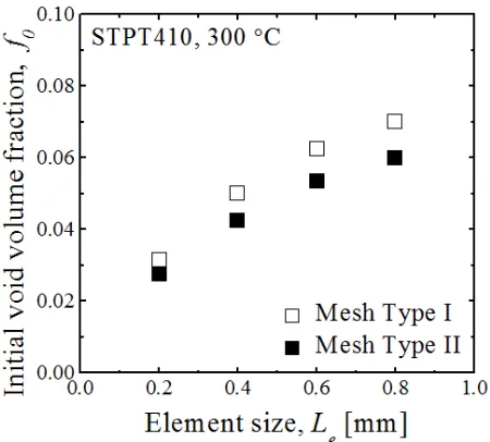
cannot provide correct predictions of both crack initiation and growth. Calibrating two parameters such as and for different element sizes would be very tedious and difficult. Therefore, in this work, the value of was calibrated as a function of the element size to fit only the initial (crack initiation) part of experimental J-R curve. Predicted J-R curves using different element size are compared with experimental data in Figure 3(b), and resulting variations of with the element size are shown in Figure 4 (indicated as the Mesh Type I). The values of for different element sizes are also given in Table 2.
(a) (b)
Figure 4. Variation of with the element size Le.
Determination of the GTN parameters using by mesh type II
The results in the previous sub-section suggest that it is difficult to reproduce both crack initiation and stable growth by calibrating only one parameter, for instance . This may be due to the fact that crack tip blunting plays an important role in crack initiation and makes crack initiation and stable crack growth different. In literature, some attempts have been made to use slightly different crack-tip mesh design, which is the subject of this sub-section.
The difference between the Mesh Type I and Mesh Type II is the shape of the first crack tip element. In the Mesh Type II, the first crack tip element splits into two parts, as shown in Figure 5(a). The calibration procedure using this type of mesh is given below.
(a) (b)
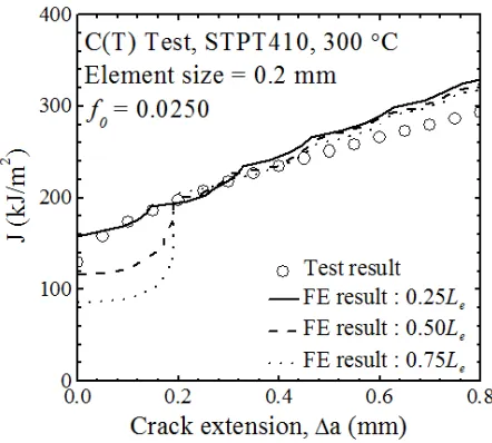
Figure 6. The effect of C in Figure 5(a) on simulated J-R curves.
To determine the size of C shown in Figure 5(a), FE damage analysis was performed using the FE mesh with Le = 0.2 mm and values of GTN model parameters given in Table 2 with = 0.025 which gives
relatively good prediction. Simulation results for various values of C are shown in Figure 6, suggesting that C = 0.25 gives smooth transition from crack initiation to stable growth.
The next step was to calibrate the value of . FE damage analysis was performed using the FE mesh with
Le = 0.2 mm and C = 0.25. Figure 7(a) shows the effect of on simulated J-R curves. The parameter
values given in Table 2 were used. Results suggest that = 0.0275 gives the best prediction, compared to the experimental data.
Then FE simulation was repeated using different element sizes. The results using Le = 0.8 mm are shown
in Figure 7(b) with several values of , suggesting that the use of = 0.06 can reproduce experimental
(a) (b)
Figure 7. The effect of on C(T) J-R simulation results using the Mesh Type II: (a) Le = 0.2 mm and (b)
Le = 0.8 mm.
Figure 8. The effect of the element size on FE J-R simulation results using the Mesh Type II.
THROUGH-WALL CRACKED PIPE TEST SIMULATION
Summary of pipe tests
Circumferential through-wall cracked pipe fracture test was conducted at 300 °C under four-point bending (Miura, 2007). The pipe material was STPT 410 carbon steel and a through-wall crack was fabricated by fatigue pre-cracking after electric discharge machining. The pipe specimens had the outer radius of 318.5 mm and the thickness of 10.3 mm. For the through-wall crack, two lengths were considered; one with a total circumferential angle of 63.6o (designated as TW-01 in this paper) and the
other with 121.4o (designated as TW-02). Quasi-static four-point bending load was applied under the
conditions. Eight-node brick elements with reduced integrations (C3D8R within ABAUQS) was uniformly spaced in the crack propagation region. At the crack tip, two types of meshes were prepared; the Mesh Type I and the Mesh Type II. The GTN parameters given in Table 1 were used with = 0.07 for the Mesh Type I, and = 0.06 for the Mesh Type II (see Table 2).
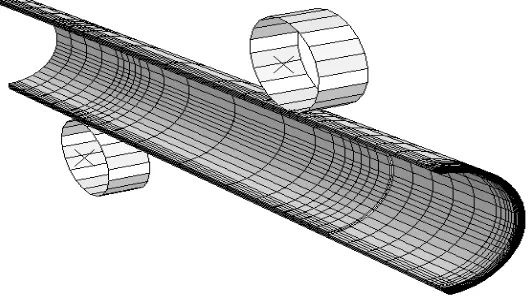
Figure 9. Typical FE mesh for pipe fracture simulation
Comparison of simulation results with experimental data
(a) (b)
Figure 10. Comparison of through-wall cracked pipe test data (TW-01) with simulated results: (a) load-LPD curve and (b) crack extension-load-LPD curve.
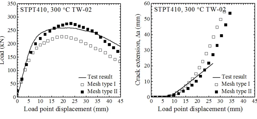
(a) (b)
Figure 11. Comparison of through-wall cracked pipe test data (TW-02) with simulated results: (a) load-LPD curve and (b) crack extension-load-LPD curve.
CONCLUSION
ABAQUS (2013), Version 6.13: User’s manual. 6.13 ed: Dassault Systems
Acharyya S., Dhar S. (2008), “A complete GTN model for prediction of ductile failure of pipe,” J Mater Sci, 43 1897-909.
Chu C, Needleman A. (1980), “Void nucleation effects in biaxially stretched sheets,” J Engng Mater Tech,
102 249-56.
Gurson AL. (1977), “Continuum theory of ductile rupture be void nucleation and growth. Part 1-yield criteria and flow rules for porous ductile media,” J Engng Mater Tech, 99 2-15.
Hojo K., Watanabe D. (2013), “Application of Gurson model to Ni-based alloy weld joint pipe with an axial or a circumferential surface flaw (phase II),” In: Proceedings of the 2013 ASME pressure vessels and piping conference, Paper PVP2013-97654
Kiran R., Khandelwal K. (2014), “Gurson model parameters for ductile fracture simulation in ASTM A992 steels,” Fat Fract Engng Mater Struct, 36 171–83.
Miura N., Miyazaki K., Hisatsune M., Hasegawa K., Kashiman K. (2007), “Ductile fracture behaviour of class 2 and 3 LWR piping and its implications for flaw evaluation criteria,” Solid State Phenom, 120 85-94
Rakin M., Gubeljak N., Dobrojevi M., Sedmak A. (2008), “Modelling of ductile fracture initiation in strength mismatched welded joint,” Eng Fract Mech, 75 3499-510.
Ruggieri C., Dotta F. (2011), “Numerical modelling of ductile crack extension in high pressure pipelines with longitudinal flaws,” Engng Struct, 33 1423-38
Schmitt W., Sun DZ., Blauel JG. (1997), “Damage mechanics analysis (Gurson model) and experimental verification of the behaviour of a crack in a weld-cladded component,” Nucl Eng Des, 174 237-46 Shatil G., Wang L. (2000), “The dependency of the local approach to fracture on the calibration of
material parameters,” In: Proceedings of European Conference Fracture, Paper ECF13
Tvergaard V., Needleman A. (1984), “Analysis of the cup cone fracture in a round tensile bar,” Acta Metall, 32 157-69.
Xue Z., Pontin M.G., Zok FW., Hutchinson JW. (2010), “Calibration procedures for a computational model of ductile fracture,” Eng Fract Mech, 77 492-509.