Copyright2001 by the Genetics Society of America
Measuring Gametic Disequilibrium From Multilocus Data
Karen L. Ayres and David J. Balding
Department of Applied Statistics, University of Reading, Reading RG6 6FN, United Kingdom Manuscript received June 20, 1999
Accepted for publication September 19, 2000
ABSTRACT
We describe a Bayesian approach to analyzing multilocus genotype or haplotype data to assess departures from gametic (linkage) equilibrium. Our approach employs a Markov chain Monte Carlo (MCMC) algo-rithm to approximate the posterior probability distributions of disequilibrium parameters. The distributions are computed exactly in some simple settings. Among other advantages, posterior distributions can be presented visually, which allows the uncertainties in parameter estimates to be readily assessed. In addition, background knowledge can be incorporated, where available, to improve the precision of inferences. The method is illustrated by application to previously published datasets; implications for multilocus forensic match probabilities and for simple association-based gene mapping are also discussed.
D
EPARTURES from gametic (or linkage) and ters have been developed (see,e.g.,Weir1979). Here, Hardy-Weinberg (HW) equilibria can provide we propose a Markov chain Monte Carlo (MCMC) clues about aspects of population histories and mating method to investigate probability distributions for ga-behavior (see,e.g.,Lewontin1974) and can be useful metic disequilibrium measures given the data. This ex-in locatex-ing disease genes (Jorde1995;Federet al.1996; tends previous work (AyresandBalding1998; Shoe-Nielsenet al.1998). They also play an important role makeret al.1998) on assessing departures from HW. in the forensic use of DNA profile evidence. Match Perhaps the most important advantage of our ap-probability calculations either rely on assumptions of proach is interpretability: the questions of interest are equilibrium (National Research Council 1996) or answered directly in terms of probabilities that can con-else allow for patterns of departures that hold in simpli- veniently be presented graphically via probability den-fied population models (Weir 1994; Balding and sity curves, providing an immediate yet detailedassess-Nichols1995;AyresandOverall1999). It is impor- ment of the variability associated with an estimate. A tant that the validity of such assumptions in actual popu- further advantage is that, since the approach is likeli-lations is verified empirically, as far as is feasible. hood based, it is statistically powerful and can incorpo-Traditional statistical treatments usually focus on test- rate a wide range of modeling assumptions. Previous ing hypotheses of equilibrium, with recent develop- treatments assume random union of gametes (RUG) to ments involving randomization tests (e.g.,Zaykinet al. infer population haplotype proportions from genotype 1995; Slatkin and Excoffier 1996). Although they data (e.g.,ExcoffierandSlatkin1995). Although we may form a useful first step, such hypothesis tests repre- also implement the RUG model in the following analy-sent a limited form of statistical inference, since the ses, we note that other models can be readily applied, tests concern only whether or not the data are consistent such as those that incorporate inbreeding measures. with equilibrium, rather than directly assessing how
The choice of prior distribution is sometimes seen as large are the departures from precise equilibrium that
a barrier to the implementation of direct probability, or inevitably exist in real populations (e.g.,Smith1970).
Bayesian, methods. We introduce a class of hierarchical In forensic applications, for example, a hypothesis of
prior distributions for the haplotype proportions, which equilibrium may be rejected with a sufficiently large
allows the scientist some flexibility either to incorporate sample, whereas a forensic scientist may nevertheless
relevant background information, if desired, or to adopt believe that the magnitude of the departure is
suffi-a relsuffi-atively “vsuffi-ague” prior. ciently small that the hypothesis of equilibrium, though
We illustrate our method by analyzing samples of ge-strictly false, is adequate for the application at hand.
notypes at two unlinked loci and at three linked loci. Point estimation methods for disequilibrium
parame-We also briefly discuss its application to forensic identi-fication, and to haplotype data and simple disequilib-rium gene mapping. Computer programs (C code) for Corresponding author:David J. Balding, Department of Applied
Statis-the MCMC algorithms are available from Statis-the authors tics, University of Reading, P.O. Box 240, Earley Gate, Reading RG6
6FN, United Kingdom. E-mail: [email protected] on request.
METHODS Measures of gametic disequilibrium not based onDij have also been proposed.Smouse(1974) specifies a log-Measures of gametic disequilibrium:Genetic
equilib-linear model for thehij, with allele-specific parameters rium corresponds to statistical independence, and many
aiandbj, and an interaction termcijthat can be employed authors (see,e.g.,Weir1979) measure gametic
disequi-as an alternative toDij.Weir(1996, pp. 127–133) details librium in terms of the differences between population
a closely related multiplicative model and extends the haplotype proportions and the values that would be
analysis to genotype data. expected under equilibrium, given the allele
propor-Here, we focus onD⬘ as a summary measure of ga-tions. Following this approach, for a two-locus haplotype
metic disequilibrium (together with an extension D″, consisting of allelesAiandBj, we introduce the notation
introduced below). This measure is widely used and, although it suffers from the interpretability drawbacks Dij⫽ hij⫺ piqj, (1)
described above, there seems to be no univariate mea-where hij denotes the population proportion of haplo- sure that avoids such difficulties. When interest focuses typeAiBj, whilepi⫽Rjhijandqj⫽Rihij, the proportions on gametic disequilibrium due to linkage, such as in of, respectively, allelesAiandBj. “simple” genetic mapping, then a natural criterion for The range of Dij depends onpi andqj, which makes choosing between disequilibrium measures is correla-cross-locus and cross-population comparisons difficult. tion with physical distance and Devlin and Risch To alleviate this problem, Lewontin (1964) defined (1995) find thatD⬘has good properties in that setting. the normalized difference, with range [⫺1, 1], by Random union of gametes model:When only geno-type counts are available, a model is required to relate D⬘ij ⫽Dij/Dmax,
the hij to genotype proportions, which then implies a model for theDij.For two loci at which the population whereDmaxis
proportion of genotype AiAi⬘BjBj⬘ is denoted pii⬘jj⬘ (with iⱕi⬘andjⱕj⬘), perhaps the simplest plausible model min(piqj, (1⫺pi)(1⫺qj)) ifDij ⬍0
min(pi(1⫺qj), (1⫺ pi)qj) ifDij ⬎0. assumes RUG:
When there are only two alleles at each locus, there is a unique value of|D⬘ij|. Otherwise, it is usually of interest
to have a summary measure of the gametic disequilib- pii⬘jj⬘⫽
h2
ij ifi⫽i⬘,j⫽j⬘ 2hijhij⬘ ifi⫽i⬘,j⬍j⬘
2hijhi⬘j ifi⬍i⬘,j⫽j⬘ 2hijhi⬘j⬘⫹ 2hi⬘jhij⬘ ifi⬍i⬘,j⬍j⬘. (3)
rium between the two loci;Hedrick(1987) proposed
D⬘ ⫽
兺
i兺
jpiqj|D⬘ij|. (2)
Inbreeding and selection, for example, will invalidate this model: haplotype proportions will be incorrectly The range ofD⬘is [0, 1], independent of thepiandqj.
estimated because no allowance is made for the depen-However, there remain difficulties in interpreting the
dence of haplotypes within multi locus genotypes. How-value of D⬘.Lewontin(1988) noted that values ofD⬘
ever, for human populations and approximately neutral at different loci and in different populations tend to
loci, the effect on inference should be negligible, and vary with the values of thepiandqj, so that the problem
so the RUG assumption may be reasonable in such cases. of cross-locus and cross-population comparisons is not
The log-likelihood for a random sample of genotypes fully overcome by use ofD⬘.
is obtained by substituting (3) into the multinomial log-Moreover, in practice the range of values ofD⬘
consis-likelihood function, tent with gametic equilibrium is not readily apparent
and can vary from locus to locus. Under equilibrium, logL⫽
兺
nii⬘jj⬘log(pii⬘jj⬘), (4) eachDij, and henceD⬘, takes value zero. However, just
as a2goodness-of-fit statistic is unlikely to be very close where then
ii⬘jj⬘are the observed genotype counts. The to zero even when the model is valid, so estimates ofD⬘ maximum-likelihood (ML) estimateshˆijcan then be ob-based on data from equilibrium populations are un- tained by maximizing logLusing any suitable method, likely to be very close to zero (furthermore, variances such as the expectation-maximization (EM) algorithm ofD⬘are difficult to calculate; seeZapataet al.1997). ofExcoffierandSlatkin(1995). Substitution of the Insight into whether or not the data are consistent with hˆij into (1) and (2) then leads to point estimates Dˆ⬘ij gametic equilibrium can be gained by reanalyzing them andDˆ⬘.
sponding to no background information about haplo- andj, respectively. (Conceptually,␣i andjmight be thought of as metapopulation allele proportions.) A type proportions. However, a uniform prior for thehij
tractable family of prior distributions for thehijwould does not correspond to an uninformative prior forD⬘,
then be the Dirichlet family with parameters ␣ij, and the level of informativeness is fixed and cannot be
whereis a constant, so that eachhijhas prior expecta-controlled. Moreover, the uniform-on-haplotypes prior
tion and variance given by does not encapsulate the fact that haplotypes are
com-posed of alleles and hence, for example, theh1j,j⬆ 1
E[hij]⫽ ␣ij, Var[hij]⫽
␣ij(1 ⫺ ␣ij) 1⫹ . (5) and thehi1, i⬆ 1 are informative about p1and q1 and
thus may well be informative abouth11.
Suppose that information was available in advance, Under this assumption, thepiand theqjare also Dirich-perhaps from surveys in other populations, which indi- let, with parameters␣iandj, respectively. Ifis large thenhij,pi, andqjwill be close to, respectively, ␣ij,␣i, cated that pi and qj were likely to be close to, say, ␣i
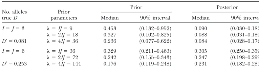
TABLE 1
Medians and equal-tailed 90% intervals of the prior and posterior distribution forDⴕshown in Figure 1
Prior Posterior
No. alleles Prior
trueD⬘ parameters Median 90% interval Median 90% interval
I⫽J⫽3 ⫽IJ⫽9 0.453 (0.132–0.952) 0.090 (0.030–0.182)
⫽2IJ⫽18 0.327 (0.102–0.825) 0.088 (0.031–0.180) D⬘ ⫽0.081 ⫽4IJ⫽36 0.236 (0.077–0.622) 0.084 (0.028–0.172)
I⫽J⫽6 ⫽IJ⫽36 0.329 (0.211–0.463) 0.305 (0.250–0.359)
⫽2IJ⫽72 0.242 (0.155–0.343) 0.247 (0.198–0.299) D⬘ ⫽0.253 ⫽4IJ⫽144 0.176 (0.119–0.248) 0.231 (0.182–0.281)
andj, and hence the implied prior forDijwill be peaked Hastings type (Metropoliset al.1953;Hastings1970). At each iteration of the algorithm, a decision is made at zero, implying little gametic disequilibrium.
Decreas-ing the value of makes strong disequilibrium more whether to keep the current vector of parameter values or reject it in favor of a new vector. The accept/reject probable (the tails of the implied prior distribution for
Dijare longer). decision is made in such a way that the proportion of iterations at which the current vector lies in any region The sum of the Dirichlet parameters provides a
mea-sure of the information conveyed by the distribution. of the parameter space approximates the probability that the true parameter vector lies in that region, with Choosingso that the average of the␣ijis one would
give a distribution that has the same information content the approximation becoming more accurate as the num-ber of iterations increases. Further details of the MCMC as the uniform (for which all the parameters equal one)
and may provide a reasonable vague prior for thehij. algorithm are given in theappendix.
Figure 1 shows the posterior density curves for D⬘, This framework for specifying a prior distribution for
hijdoes not require that␣iandjbe specified precisely. approximated via the MCMC algorithm, given two sam-ples of two-locus genotypes simulated under the RUG Instead, they can be assigned probability distributions,
leading to a hierarchical prior model. Below, we adopt model withD⬘ ⫽0.081 (three alleles) and D⬘ ⫽0.253 (six alleles). Three prior distributions were employed, independent uniform distributions for the ␣i and j,
although background information could in practice be shown as dotted curves. Key quantiles of the prior and posterior distributions are given in Table 1.
incorporated into more informative distributions.
MCMC algorithm:We implement an MCMC stochas- Even with a reasonably large sample size (200 individ-uals), D⬘ is a difficult parameter to estimate. This is tic simulation algorithm for genotype data to
approxi-mate the joint distribution of thehij, and hence of the because the data bear directly on the population geno-type proportions, whereas differences between allele gametic disequilibrium measures, under the RUG model
and the hierarchical prior distribution described above. and haplotype proportions are the quantities of interest. This difficulty is reflected by the posterior curves of The MCMC algorithm adopted is of the
Figure 1, which support a rather broad range of values and standard deviation 0.039. These values compare favorably with the MLE-based estimatesDˆ⬘, for which the forD⬘and display some sensitivity to the choice of prior.
However, in each case the posterior median is close to mean and standard deviation over these 100 simulated datasets were 0.407 and 0.040.
the true value and usually closer than the corresponding ML-based estimates (0.058 and 0.315), for which the sampling variance is difficult to calculate. Moreover,
RESULTS since D⬘ is univariate it is relatively easy to plot both
prior and posterior density curves and hence assess visu- Two unlinked loci used for forensic identification: ally the effect of the prior from the plots. Background The MCMC method was applied to the genotypes at information, when available, can be incorporated via two unlinked forensic short tandem repeat (STR) loci, the prior and may be invaluable in situations of little THO1 and TPOX, for samples of Maoris (n ⫽ 1091) data and/or many alleles. and Samoans (n⫽139) resident in New Zealand. Eight Also shown in Figure 1 are density curves averaged alleles were observed for locus THO1 and six for TPOX over 50 random permutations of the alleles, mimicking (additional alleles observed in other populations are 50 samples from populations in gametic equilibrium ignored here, although they could be incorporated into with the same allele proportions. The data with three the analysis if desired).
alleles at each locus are clearly consistent with equilib- Figure 2 shows prior ( ⫽ IJ) and posterior curves rium, but those with six alleles are not. These results for the overall measure D⬘ together with a curve ob-are in accord with thePvalues 0.56 and 0.00 obtained tained from 50 random permutations of the data (mim-from an LR-based permutation test for gametic disequi- icking equilibrium). There is a substantial overlap of librium (Slatkin andExcoffier1996). these curves, suggesting that both samples are consistent Figure 1 corresponds to a single simulated dataset. with gametic equilibrium in the underlying populations; We also applied the MCMC method (for the prior with these conclusions are in agreement with P values
ob- ⫽IJ) to 100 datasets of sizen⫽1000, simulated with tained from the LR-based permutation test (0.42 and I⫽J⫽3. The underlyinghijwere such thatD⬘ ⫽0.404. 0.13).
For each dataset we calculated the posterior median: A full multilocus match probability involves correla-tions of genes both within and between individuals (in the 100 estimated posterior medians had mean 0.403
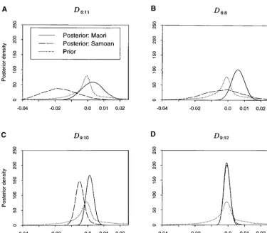
Figure 3.—Posterior densities for disequilibrium coefficients D6:11, D8:8, D9:10,
andD9:12for the Maori and
Figure 4.—Posterior densi-ties (solid curves) for pairwise disequilibrium coefficients D″ from a sample ofn⫽96 geno-types, at loci LF261 (four al-leles), LF168 (four alal-leles), and LF347 (five alleles) of the MOYO strains of theA. aegypti mosquito data of Yan et al. (1997). Point estimates (from ML estimates) are 0.492, 0.220, and 0.242. Dot-dashed curves are posterior densities aver-aged over 50 random permuta-tions of the genotypes. The prior densities (dotted curves) are based on a Dirichlet prior for the hij, with parameters 40␣ij␥k, conditional on the ␣i,
j, and␥k, which are each (mul-tivariate) uniform.
the latter case, between the defendant and an alternative is therefore important to investigate levels of gametic disequilibrium, and a selection of marginal posterior possible source of the crime scene DNA). In current
practice (see,e.g.,EvettandWeir 1998), adjustment density curves for the Dij is shown in Figure 3. All the posterior distributions support values close to zero, en-is often made for between-individual correlations at a
single locus. However, multilocus forensic match proba- couraging optimism that the effect of gametic disequi-librium on two-locus forensic match probabilities involv-bilities are usually obtained by taking the product of
the single-locus probabilities, thereby assuming inde- ing these loci may indeed be negligible.
Although these results tend to support current prac-pendence between loci. Strong gametic disequilibrium
may invalidate this assumption. tice, note that we have not simultaneously taken all relevant correlations into account. In particular, other Although THO1 and TPOX are unlinked, gametic
disequilibrium may nevertheless arise (due to founder forms of assocation may invalidate the independence of genes assumption in the match probability (seeAyres
effects, selection, or drift) and affect multilocus forensic
Figure5.—Posterior median (䊏) and central 90% posterior intervals (—) forD⬘in two populations, for the Xq25–Xq28 SNP data ofTaillon-Milleret al.(2000); marker pairs analyzed here correspond to those presented in Table 2 ofTaillon-Miller
et al.(2000). A multivariate uniform prior was used for thehij.
inbreeding). Also, forensic identification involves many from chromosome 3 of the MOYO strain of the mos-quito Aedes aegypti. For the three RFLP loci LF261, loci, often⬎10, whereas here we have considered only
the two-locus case. LF168, and LF347, they reported that the values ofD⬘ for all three pairs were significant at the 1% level. We Three linked loci:The MCMC algorithm for
approxi-mating the joint posterior of the haplotype proportions have calculated posterior density curves for D″ on the basis of their original data, as well as curves based on is readily extended to three loci. For forensic
applica-tions, we may be interested in investigating the differ- random permutations (Figure 4).
Our results suggest strong disequilibrium between LF ence hijk ⫺ piqjrk, which can be readily obtained from
the MCMC output. For other problems, simultaneous 261 and LF168, since the curve based on the randomly permuted data has little overlap with that based on the estimation of the pairwise disequilibrium measures may
be of more interest. However, multilocus systems impose observed data. In contrast, Figure 4 suggests little or no disequilibrium between the other two pairs of loci. The additional constraints on theDij. For three diallelic loci,
Robinsonet al.(1991) describe a new pairwise normal- latter conclusion differs from that ofYanet al.(1997). It is, however, consistent with the relative map positions ized measureD″ij based on these adjusted bounds and
with range [⫺1, 1]. These authors also note that addi- of the loci—LF168 is situated between LF261 and LF347, much closer to LF261 than to LF347. Although the tional loci beyond three add no further constraints on
the Dij. The multiallelic analogue of the formulas of MCMC results correctly identify LF168 and LF261 as the closest pair, disequilibrium between the other
Robinsonet al.(1991) is given in the appendix.
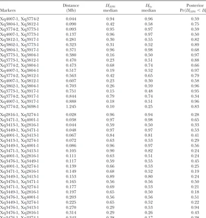
TABLE 2
Posterior summaries ofDⴕfor the analyses of Figure 5
Distance D⬘CEPH D⬘Fin Posterior
Markers (Mb) median median Pr(D⬘CEPH⬍D⬘Fin)
Xq4007-1, Xq3774-2 0.044 0.94 0.96 0.59
Xq3804-1, Xq3812-1 0.090 0.42 0.58 0.75
Xq3774-2, Xq3773-1 0.093 0.95 0.97 0.59
Xq4007-1, Xq3773-1 0.137 0.96 0.97 0.50
Xq3812-1, Xq3917-1 0.281 0.30 0.55 0.82
Xq3862-1, Xq3773-1 0.323 0.31 0.52 0.89
Xq3804-1, Xq3917-1 0.371 0.96 0.98 0.68
Xq3773-1, Xq3804-1 0.380 0.16 0.50 0.97
Xq3773-1, Xq3812-1 0.470 0.23 0.51 0.88
Xq3774-2, Xq3804-1 0.473 0.68 0.74 0.66
Xq4007-1, Xq3804-1 0.517 0.19 0.52 0.97
Xq3774-2, Xq3812-1 0.563 0.42 0.65 0.79
Xq4007-1, Xq3812-1 0.607 0.23 0.30 0.58
Xq3862-1, Xq3804-1 0.703 0.26 0.59 0.96
Xq3773-1, Xq3917-1 0.751 0.15 0.48 0.95
Xq3774-2, Xq3917-1 0.844 0.79 0.74 0.34
Xq4007-1, Xq3917-1 0.888 0.18 0.51 0.96
Xq3774-2, Xq3698-1 1.245 0.10 0.25 0.83
Xq2816-1, Xq3274-1 0.028 0.96 0.94 0.28
Xq3471-1, Xq4001-1 0.038 0.97 0.98 0.65
Xq3413-1, Xq2816-1 0.044 0.59 0.50 0.33
Xq3449-1, Xq3471-1 0.048 0.97 0.97 0.53
Xq4001-1, Xq3413-1 0.067 0.84 0.81 0.41
Xq3413-1, Xq3274-1 0.072 0.63 0.53 0.29
Xq3449-1, Xq4001-1 0.086 0.96 0.97 0.56
Xq3471-1, Xq3413-1 0.105 0.90 0.82 0.24
Xq4001-1, Xq2816-1 0.111 0.63 0.51 0.24
Xq3476-1, Xq3449-1 0.117 0.59 0.55 0.45
Xq4001-1, Xq3274-1 0.139 0.66 0.53 0.25
Xq3471-1, Xq2816-1 0.149 0.68 0.52 0.19
Xq3449-1, Xq3413-1 0.153 0.89 0.80 0.24
Xq3476-1, Xq3471-1 0.165 0.56 0.56 0.50
Xq3471-1, Xq3274-1 0.177 0.69 0.53 0.21
Xq3449-1, Xq2816-1 0.197 0.65 0.50 0.18
Xq3476-1, Xq4001-1 0.203 0.56 0.56 0.51
Xq3449-1, Xq3274-1 0.225 0.65 0.52 0.22
Xq3476-1, Xq3413-1 0.270 0.29 0.53 0.94
Xq3476-1, Xq2816-1 0.314 0.29 0.26 0.43
Xq3476-1, Xq3274-1 0.342 0.28 0.17 0.28
Posterior medians (based on 1000 sampled values) forD⬘in two populations (CEPH,n⫽92; Finland (Fin), n⫽100), for the Xq25–Xq28 SNP data ofTaillon-Milleret al.(2000); also shown is the probability thatD⬘ in the CEPH population is less thanD⬘in the Finnish population. Marker pairs analyzed here correspond to those presented in Table 2 ofTaillon-Milleret al.(2000) and are ordered by distance between the markers. A multivariate uniform prior was used for thehij.Each entry is based on 1000 values sampled from the posterior distribution ofD⬘.
where N⬅ {nijk} denotes the sample haplotype counts markers on the basis of the joint posterior distribution of
and␣, , and ␥are vectors of hyperparameters speci-theD″cannot be achieved with confidence, the correct
fying prior distributions for the population allele pro-order being assigned a probability of 42%.
portions at the three loci. Haplotype data:In some cases haplotype counts may
A method for sampling from this distribution is given be available, simplifying the direct probability approach.
in theappendix, together with a summary of implica-For example, for three-locus haplotypeshijkand a
hierar-tions for disequilibrium mapping. However, we focus chical prior, we have
DISCUSSION parameterskijis implemented for thehij.When the
likeli-hood is multinomial, the posterior distribution for the The direct probability, or Bayesian, approach devel-hij will again be Dirichlet with parametersnij ⫹kij, and oped here permits interpretable visual answers to the a sample from this distribution can be obtained by stan- question of interest about disequilibrium parameters. dard random number generation (see,e.g., Appendix Moreover, it can readily incorporate complex models
A ofGelmanet al.1995). and background knowledge about a population, when
Taillon-Miller et al. (2000) analyzed several pairs available. For a discussion of the advantages of Bayesian of single nucleotide polymorphism (SNP) markers in approaches to problems in genetics, seeShoemakeret the human Xq25–Xq28 region for three populations al.(1999). We have also developed a family of hierarchi-[general European (CEPH), Finnish, and Sardinian]. cal prior distributions that allow the scientist some flex-They found significantPvalues (P⬍ 0.001, from a2
ibility in specifying background knowledge. test for gametic equilibrium) for markers separated by
Zapataet al.(1997) note that point estimates of D⬘ij up toⵑ900 kb. They also found that, in general, point
are frequently reported without a corresponding mea-estimates of disequilibrium measures (such asD⬘) did
sure of variability (such as the standard error), which not differ greatly between the large outbred population
can complicate comparisons over loci and populations. (represented by the CEPH sample) and the genetically
However, the calculation of Var(D⬘ij) is complicated by isolated populations of Finland and Sardinia. These
re-the different rescaling of positive and negative values sults were consistent with an STR analysis of similar
in the definition ofD⬘ij. Zapataet al.derived an approxi-populations (Eaves et al. 2000), though both conflict
mation to Var(D⬘ij) for biallelic loci only. Our direct with the suggestion that genetically isolated populations
probability approach provides an approximation not tend to exhibit higher levels of disequilibrium and are
just for the variance of (multiallelic)D⬘ijandD⬘but for therefore more useful for disease gene mapping (see,
their entire posterior distributions. A particular advan-e.g.,Wright et al. 1999). In summarizing the
conclu-tage is that the posterior intervals obtained can be di-sions ofTaillon-Milleret al.(2000) andEaveset al.
rectly interpreted in terms of probabilities, unlike stan-(2000),Boehnke (2000) argues that the levels of
dis-dard confidence intervals that are routinely provided equilibrium observed appeared slightly stronger in the
for some point estimates, which do not have such a isolates than in the general mixed populations.
direct interpretation. We have reanalyzed the CEPH and Finnish SNP data
There are no theoretical limits to the number of loci ofTaillon-Milleret al.(2000), implementing a
multi-that can be analyzed simultaneously. However, for a variate uniform prior forhij for each pair of markers
fixed sample size, the information contained in the data analyzed. This distribution imposes a prior belief that
decreases as the number of loci increases, and, as for none of the alleles is very rare [the implied prior for
hypothesis testing, useful inferences are usually not fea-thepiandqjis Beta(2,2)], which is reasonable for these
sible for more than about three loci. markers as they have been selected on the basis of
poly-We thank the following for kindly providing the data analyzed in morphism. Results are shown in Figure 5: posterior
me-this study: John Buckleton (human STR data), Guiyun Yan (mosquito dians and 90% intervals for the two populations are
data), Patty Taillon-Miller, and Pui-Yan Kwok (SNP data). We thank plotted against physical distance. Laurent Excoffier for helpful comments on an earlier draft, as well The measure of variability provided by our MCMC as two anonymous referees. Work was supported in part by the UK approach allows more careful comparison of the levels Biotechnology and Biological Sciences Research Council, under grant
45/G09617. of disequilibrium across the populations analyzed. For
almost all of the marker pairs given in Table 2, the posterior 90% intervals from the two populations
over-lap substantially, indicating that there is little evidence LITERATURE CITED of any difference across the populations. This is
quanti-Ayres, K. L.,1998 Measuring genetic correlations within and be-fied in Table 2, which gives the posterior probability tween loci, with implications for disequilibrium mapping and for each marker pair that D⬘ is larger in the Finnish forensic identification. Ph.D. Thesis, The University of Reading,
Reading, UK. population than in the CEPH population: these
proba-Ayres, K. L.,2000 A two-locus forensic match probability for subdi-bilities exceed 90% for only a handful of markers, and
vided populations. Genetica108:137–143.
in no case exceed 97%. (Note the values ofD⬘ across Ayres, K. L.,andD. J. Balding,1998 Measuring departures from Hardy-Weinberg: a Markov chain Monte Carlo method for esti-closely linked markers are not independent.)
mating the inbreeding coefficient. Heredity80:769–777. Our results therefore quantify the observation made
Ayres, K. L.,andA. D. J. Overall,1999 Allowing for within-subpop-by Taillon-Miller et al. (2000) that disequilibrium ulation inbreeding in forensic match probabilities. Forensic Sci.
Int.103:207–216. levels were similar across the populations. The data
pro-Balding, D. J.,andR. A. Nichols,1995 A method for quantifying vide little evidence that gametic disequilibrium is higher
differentiation between populations at multi-allelic loci and its in the Finnish population than in the general European implications for investigating identity and paternity. Genetica96:
Best, N. G., M. K. CowlesandS. K. Vines,1995 CODA Manual strains selected for refractoriness to a malaria parasite. J. Hered. 88:187–194.
Version 0.30.MRC Biostatistics Unit, Cambridge, UK.
Zapata, C., G. AlvarezandC. Carollo,1997 Approximate vari-Boehnke, M.,2000 A look at linkage disequilibrium. Nat. Genet.
ance of the standardized measure of gametic disequilibriumD⬘. 25:246–247.
Am. J. Hum. Genet.61:771–774. Brooks, S. P., 1998 Markov chain Monte Carlo method and its
Zaykin, D., L. A. ZhivotovskyandB. S. Weir,1995 Exact tests for application. Statistician47:69–100.
association between alleles at arbitrary numbers of loci. Genetica Devlin, B.,andN. Risch,1995 A comparison of linkage
disequilib-96:169–178. rium measures for fine-scale mapping. Genomics29:311–322.
Eaves, I. A., T. R. Merriman, R. A. Barber, S. Nutland, E. Tuomi- Communicating editor:G. A. Churchill lehto-Wolfet al., 2000 The genetically isolated populations
of Finland and Sardinia may not be a panacea for linkage disequi-librium mapping of common disease genes. Nat. Genet.25:320–
323. APPENDIX
Evett, I. W.,andB. S. Weir,1998 Interpreting DNA Evidence: Statistical
Genetics for Forensic Scientists.Sinauer, Sunderland, MA. MCMC algorithm for genotype data: Metropolis-Has-Excoffier, L.,andM. Slatkin,1995 Maximum-likelihood estima- tings algorithms are methods for generating a sample
tion of molecular haplotype frequencies in a diploid population.
from an arbitrary probability distribution⌸(with proba-Mol. Biol. Evol.12:921–927.
bility density function) by constructing a Markov chain Feder, J. N., A. Gnirke, W. Thomas, Z. Tsuchihashi, D. A. Ruddy
et al., 1996 A novel MHC class I-like gene is mutated in patients whose stationary distribution is ⌸. If the current state with hereditary haemochromatosis. Nat. Genet.13:399–408.
of the chain isx, a candidate new statex⬘is chosen with Gelman, A., J. B. Carlin, H. S. SternandD. B. Rubin,1995 Bayesian
probability density q(x⬘|x). The candidate is accepted Data Analysis.Chapman and Hall, London.
Hastings, W. K.,1970 Monte Carlo sampling methods using Markov with probability chains and their applications. Biometrika57:97–109.
Hedrick, P. W., 1987 Gametic disequilibrium measures: proceed
with caution. Genetics117:331–341. min
冢
(x⬘)q(x|x⬘)(x)q(x⬘|x), 1
冣
, Jorde, L. B.,1995 Linkage disequilibrium as a gene-mapping tool.Am. J. Hum. Genet.56:11–14.
Lewontin, R. C.,1964 The interaction of selection and linkage. I. otherwise the current statexis retained. A key feature General considerations; heterotic models. Genetics49:49–67. of these algorithms is that need only be specified Lewontin, R. C.,1974 The Genetic Basis of Evolutionary Change.
Co-up to a normalizing constant, and so high-dimensional lumbia University Press, New York.
probability distributions can often be successfully han-Lewontin, R. C.,1988 On measures of gametic disequilibrium.
Ge-netics120:849–852. dled. Although the states of the chain are correlated,
Metropolis, N., A. W. Rosenbluth, M. N. Rosenbluth, A. H.
selecting every kth iteration, after an initial “burn-in” TellerandE. Teller,1953 Equation of state calculations by
period of length b, can lead to approximate random fast computing machines. J. Chem. Phys.21:1087–1092.
National Research Council,1996 The Evaluation of Forensic DNA samples from ⌸when suitable choices are made fork Evidence, NRC2. National Academy Press, Washington, DC.
andb.SeeBrooks(1998) for an introduction to MCMC Nielsen, D. M., M. G. EhmandB. S. Weir,1998 Detecting
marker-algorithms. disease association by testing for Hardy-Weinberg disequilibrium
at a marker locus. Am. J. Hum. Genet.63:1531–1540. For the algorithm implemented here,is the joint Robinson, W. P., M. A. AsmussenandG. Thomson,1991
Three-posterior density function of thehij. For two loci, each locus systems impose additional constraints on pairwise
disequil-candidatex⬘ differs fromxat a randomly chosen pair bria. Genetics129:925–930.
Shoemaker, J., I. PainterandB. S. Weir,1998 A Bayesian character- of thehij, sayhrsandhwz.A proposal valueh⬘rsis chosen ization of Hardy-Weinberg disequilibrium. Genetics149:2079–
uniformly in the interval 2088.
Shoemaker, J., I. PainterandB. S. Weir,1999 Bayesian statistics in
(max(0,hrs⫺ε), min(hrs⫹ε,hrs⫹ hwz)), genetics: a guide for the uninitiated. Trends Genet.15:354–358.
Slatkin, M.,andL. Excoffier,1996 Testing for linkage
disequilib-and h⬘wz ⫽ hwz ⫹ hrs ⫺ h⬘rs. The (positive) value of ε is rium in genotypic data using the Expectation-Maximization
algo-rithm. Heredity76:377–383. chosen to prevent proposed values from being rejected Smith, A. F. M.,andJ. M. Bernardo,1994 Bayesian Theory.Wiley, too often, which would result in slow movement of the
Chichester, UK.
chain around the sample space. Smith, C. A. B.,1970 A note on testing the Hardy-Weinberg law.
Ann. Hum. Genet.33:377–383. Slow convergence and poor mixing can arise in the Smouse, P. E.,1974 Likelihood analysis of recombinational disequi- presence of many alleles and/or loci. No difficulties
librium in multiple-locus gametic frequencies. Genetics76:557–
were experienced with the examples discussed here that 565.
could not reasonably be overcome by choosing suitably Taillon-Miller, P., I. Bauer-Sardin˜ a, N. L. Saccone, J. Putzel,
T. Laitinenet al., 2000 Juxtaposed regions of extensive and large values forkandb.A burn-in ofb⫽30,000 iterations minimal linkage disequilibrium in human Xq25 and Xq28. Nat.
was found to be adequate for the two-locus algorithm Genet.25:324–328.
(50,000 for three loci), with everyk⫽200th (300) itera-Weir, B. S.,1979 Inferences about linkage disequilibrium.
Biomet-rics35:235–254. tion output (these values having been determined by
Weir, B. S.,1994 The effects of inbreeding on forensic calculation.
the inspection of sequential and autocorrelation plots Ann. Rev. Genet.28:597–621.
of the output for initial runs). The output of each run Weir, B. S.,1996 Genetic Data Analysis II.Sinauer, Sunderland, MA.
Wright, A. F., A. D. CarothersandM. Pirastu,1999 Population underlying the figures and tables was analyzed with the choice in mapping genes for complex diseases. Nat. Genet.23: MCMC diagnostic computer package CODA (Best et 397–404.
al.1995), which indicated satisfactory convergence and Yan, G., B. M. ChristensenandD. W. Severson,1997 Comparisons
algorithm to the data, 5000 values were output (1000 est to the disease locus should exhibit higher levels of disequilibrium than those that are far away (e.g.,Jorde
for the permuted data).
MCMC algorithm for haplotype data:For three-locus 1995). Devlin and Risch (1995) detailed the use of point estimates of disequilibrium for inferring the clos-haplotype data, assuming a multinomial log likelihood
for thehijk(given hyperparameters␣,, and␥), together est of a number of biallelic markers (identifying the marker with the highest observed disequilibrium value with a Dirichlet prior distribution, after observing the
nijkthehijkhave a Dirichlet distribution with parameters as the closest). The direct probability approach, imple-menting the methods outlined above, adds a degree nijk ⫹ ␣ij␥k. A posterior sample from p({hijk}|␣, , ␥,
N) can therefore be readily obtained using standard of interpretability to simple disequilibrium mapping, assigning probabilities to the event that a marker is methods for the Dirichlet distribution (see,e.g.,
Appen-dix A ofGelman et al.1995). To obtain a distribution closest to the disease locus—seeAyres(1998) for fur-ther details.
for the hijk that does not involve ␣, , and ␥, we can
Multiallelic three-locus normalized measures:The fol-employ (6) together with a method of simulating from
lowing bounds apply to theDij for two loci in a three-p(␣, , ␥|N). A number of approaches are available,
locus system (disequilibrium measures for the other lo-and details of an MCMC algorithm are given here.
cus pairs are denotedDikandDjk), The target distribution for the MCMC algorithm is
p(␣, , ␥|N), the probability density function of the
Dijmin⫽max{⫺piqj,⫺(1 ⫺pi)(1⫺qj), ⫺m1,⫺m2}
hyperparameters ␣, , and ␥ given the data N. The
likelihoodp(N|␣,,␥) is of a standard form known as Dijmax⫽min{pi(1 ⫺qj), (1⫺pi)qj,M1,M2},
the multinomial-Dirichlet (SmithandBernardo1994,
where p. 135), and by Bayes theorem we can write
m1⫽piqjrk⫹(1 ⫺pi)(1⫺ qj)(1⫺rk)⫹Dik⫹Djk p(␣,,␥|N)⫽cp(␣,,␥)
兿
I
i⫽1
兿
J
j⫽1
兿
K
k⫽1
⌫(nijk⫹ ␣ij␥k)
⌫(␣ij␥k) ,
m2⫽piqj(1 ⫺rk)⫹(1⫺ pi)(1⫺ qj)rk⫺Dik⫺Djk
(7) M1⫽pi(1⫺ qj)rk⫹(1 ⫺pi)qj(1⫺rk)⫹Dik⫺Djk
M2⫽pi(1⫺ qj)(1⫺rk)⫹(1⫺ pi)qjrk⫺Dik⫹Djk, in which c is a constant (and hence does not need
to be known here) andp(␣, , ␥) denotes the prior
which are analogous to equations (12, a and b) and distribution for the hyperparameters, assumed here to
(13, a–d) of Robinson et al. (1991). The normalized be the product of multivariate uniforms so thatp(␣,,
parametersD″ij defined by these authors are then given
␥) is also a constant.
by A suitable Metropolis-Hastings algorithm can proceed
as follows: first select a locus l, chosen uniformly at random. Suppose for notational convenience that␣is the hyperparameter vector corresponding to the chosen locusl, then choose two elements of␣, say ␣vand␣w. The proposal␣⬘v is chosen uniformly at random in the interval
D″ij ⫽
Dij
Dijmax
ifDij⬎ 0 andDijmin ⱕ0 Dij⫺Dijmin
Dijmax⫺Dijmin
ifDij⬎0 and Dijmin⬎ 0 Dij
⫺Dijmin
ifDij⬍0 and Dijmaxⱖ 0 Dij ⫺Dijmax
Dijmax⫺Dijmin
ifDij⬍0 and Dijmax⬍ 0. (max(0,␣v⫺ε), min(␣v⫹ε,␣v⫹ ␣w)), (8)
whereεis again a tuning parameter chosen to ensure that proposal values are not rejected either too fre-quently or too rarely. Finally,␣⬘wis assigned value␣w⫹
␣v⫺ ␣⬘v.
This algorithm, and modifications of it, can be useful TheD″ij can be interpreted as the amount by which |Dij| in the location of disease loci via simple disequilibrium exceeds its minimum value (given its sign), divided by mapping. Briefly, under the assumption of a single dis- its range. The overall pairwise measureD″is calculated