ABSTRACT
UNDERWOOD, DANIEL J. Simulation Optimization of Prostate Cancer Screening Using a Parallel Genetic Algorithm. (Under the direction of Dr. Brian T. Denton.)
We develop a parallel simulation-optimization method to find near optimal PSA screening policies based on the mean expected quality adjusted life years (QALYs) of a large population. In contrast to mortality-based indicators such as life expectancy, QALYs are informed by treatment side-effects, chronic disease, and other non-fatal degradations to quality of life. We seek an optimal balance of the benefits of early detection of prostate cancer and the reduction in QALYs associated with overdiagnosis.
A screening policy’s impact on QALYs is examined by using a non-stationary Markov model to simulate a patient’s progression through health-states, PSA levels, and treatment. The simulation model is embedded within a parallel genetic algorithm (GA) to search the space of possible PSA screening policies for unrealized optimal policies. A ranking and selection scheme is employed by the GA in order to manage the computational budget. The ranking and selection scheme is designed to balance the trade-off between exploring the large policy space and achieving statistical confidence in the simulation output that is necessary to meaningfully distinguish different screening policies.
c
Copyright 2010 by Daniel J. Underwood
Simulation Optimization of Prostate Cancer Screening Using a Parallel Genetic Algorithm
by
Daniel J. Underwood
A thesis submitted to the Graduate Faculty of North Carolina State University
in partial fulfillment of the requirements for the Degree of
Master of Science
Operations Research
Raleigh, North Carolina
2010
APPROVED BY:
Dr. James R. Wilson Dr. John W. Baugh
DEDICATION
BIOGRAPHY
ACKNOWLEDGEMENTS
TABLE OF CONTENTS
List of Tables . . . vii
List of Figures . . . .viii
Chapter 1 Introduction . . . 1
Chapter 2 Background on Prostate Cancer Screening . . . 4
Chapter 3 Literature Review . . . 7
3.1 Prostate Cancer Modeling . . . 7
3.2 Simulation Optimization . . . 8
3.2.1 Ranking and Selection . . . 8
3.2.2 Genetic Algorithms . . . 9
3.2.3 Parallel Computing . . . 10
3.3 Contribution to the Literature . . . 10
Chapter 4 Simulation Model . . . 12
4.1 PSA Screening . . . 14
4.2 Accumulation of Reward . . . 15
4.3 Core Health-State Transition Probabilities . . . 15
4.4 Computing Platforms . . . 17
4.5 Numerical Results . . . 18
4.5.1 Data and Model Parameters . . . 18
4.5.2 Discounting QALYs . . . 18
4.5.3 Evaluation of Proposed Screening Policies . . . 19
4.6 Conclusions . . . 22
Chapter 5 Optimization of PSA-Threshold Screening Policies. . . 23
5.1 Optimization Model . . . 24
5.2 Genetic Algorithm . . . 25
5.3 Results . . . 32
5.3.1 Experimental Evaluation of Genetic Algorithm . . . 32
5.3.2 Experimental Evolution of Genetic Algorithm . . . 35
5.3.3 Optimal PSA Screening Policies . . . 35
5.3.4 Clinically Relevant Screening Policies . . . 37
5.3.5 Upper Bounds on the Optimal Policy . . . 40
5.3.6 Multiple Biopsy . . . 40
5.3.7 Sensitivity Analysis . . . 44
Chapter 6 Conclusion . . . 48
6.1 Summary of Conclusions . . . 48
6.2 Implications for Research and Practice . . . 49
6.3 Potential Future Research . . . 50
LIST OF TABLES
Table 4.1 Parameters for transition probability matrices . . . 16
Table 4.2 Reward parameters used in evaluating proposed screening policies . . . 18
Table 4.3 Transition probabilities used in evaluating proposed screening policies . . . 19
Table 5.1 Precision and running time analysis . . . 32
Table 5.2 Comparison between the best GA policy and the optimal POMDP policy [47] 40 Table 5.3 Sensitivity analysis on parameters of reward function in terms of the effect on the entire U.S. male population . . . 44
Table 5.4 Sensitivity analysis on parameters of reward function in terms of the effect on the subpopulation of U.S males who ultimately develop cancer . . . 45
Table 5.5 Recommendation for PSA-threshold screening policy . . . 46
Table 6.1 Comparison of the expected QALYs for the Ross policies . . . 48
LIST OF FIGURES
Figure 2.1 Receiver Operating Characteristic (ROC) curve illustrating the imperfect nature of PSA testing based on longitudinal data for a regional population
in Rochester, MN . . . 6
Figure 4.1 Transitions between health-states . . . 13
Figure 4.2 States considered following treatment . . . 13
Figure 4.3 Histogram of PSA observations from empirical data . . . 14
Figure 4.4 Sensitivity analysis on parameters of reward function for Ross policies . . 19
Figure 4.5 Ross results comparison for entire U.S. male population . . . 20
Figure 4.6 Ross results comparison for subpopulation of U.S. males who ultimately develop prostate cancer . . . 21
Figure 4.7 Comparison between the Ross policies’ effect on the entire U.S. male population and the subpopulation of U.S. males who ultimately develop prostate cancer . . . 21
Figure 5.1 High-level model of GA . . . 25
Figure 5.2 Example roulette wheel illustration . . . 27
Figure 5.3 Single-point crossover illustration . . . 29
Figure 5.4 Two-point crossover illustration . . . 29
Figure 5.5 Convergence of mean as sample size increases . . . 33
Figure 5.6 Comparison of crossover methods . . . 34
Figure 5.7 Comparison of selection methods . . . 34
Figure 5.8 Comparison of mutation rates . . . 35
Figure 5.9 Evolution of GA showing period of sharpest incline in fitness improvement from generation to generation . . . 36
Figure 5.10 Evolution of GA showing convergence to optimum . . . 36
Figure 5.11 Optimal PSA screening policy discovered by GA in raw form . . . 37
Figure 5.12 Optimal PSA screening policy discovered by GA in simplified form . . . . 38
Figure 5.13 Comparing the Ross policies to the optimal GA policy (both the raw version and the simplified version) in terms of the effect on the entire U.S. male population . . . 39
Figure 5.14 Comparing the Ross policies to the optimal GA policy in terms of the effect on the subpopulation of U.S. males who ultimately develop prostate cancer . . . 39
Figure 5.15 Optimal PSA screening policy under maximum of 3 biopsies per patient discovered by GA in raw form . . . 41
Figure 5.16 Optimal PSA screening policy under maximum of 3 biopsies per patient discovered by GA in simplified form . . . 41
CHAPTER
1
Introduction
Prostate cancer is one of the most common cancers affecting males. Statistics show for males in the United States during 2009 that prostate cancer was responsible for 25% of new cancers and 9% of deaths from cancer (excluding skin cancers) [28]. Clinicians screen for prostate cancer by monitoring the serum-level of prostate-specific antigen (PSA) in males. PSA is a protein produced by cells in the prostate gland; PSA is also a continuous biomarker that is correlated with prostate cancer. Males typically have low levels of PSA in the their blood. High PSA levels often point to the existence of cancerous cells in the prostate. However, PSA screening is an imperfect test, resulting in false positives, because increased PSA levels can result from benign prostatic hyperplasia (BPH), also known as benign prostate enlargement. Furthermore, because the all-cause mortality rate increases with age, and because prostate cancer is a slow growing cancer, PSA screening loses its utility in older patients. The age at which to discontinue screening is central to the debate on PSA screening.
biopsy is 0.8.
Because the treatment options following a positive PSA test can cause serious negative side-effects [40], reducing the likelihood of false positives is naturally of great interest to researchers, patients, and practitioners.
Studies on the value of PSA screening for prostate-cancer detection have produced mixed results. The first report from the Prostate, Lung, Colorectal, and Ovarian (PLCO) Cancer Screening Trial on prostate-cancer mortality indicates that PSA screening doesnot effectively reduce the rate of death from prostate cancer [4]. Results from The European Randomized Study of Screening for Prostate Cancer, on the other hand, indicate that PSA screeningdoes reduce the rate of death from prostate cancer [41]. The heterogeneity of results from controlled trials on the impact of PSA screening makes this subject particularly suitable for simulation analysis.
The problem of determining the best PSA screening policy is controversial and difficult to solve. Physicians typically consider a discrete set of clinically relevant ranges of PSA. Assuming arguendo that there are a total of 5 different possible PSA threshold levels (in reality PSA is a continuous measure), that screening may take place no more frequently than every 3 months, and that screening may begin at age 40, then there are 5160 = 6.8×10111 possible screening policies. Obviously it is not possible to conduct randomized controlled trials to evaluate and compare all possible screening policies. Even using a computer to systematically simulate and evaluate all the possible screening policies is not feasible (e.g. if a computer can evaluate 1,000,000 screening policies per second, it would take 2.2×1098 years to evaluate all policies).
The problem of determining the best PSA screening policy demands sophisticated optimiza-tion techniques. This optimizaoptimiza-tion problem is difficult for multiple reasons. Because the problem space is stochastic and non-convex, methods such as stochastic linear programming and dynamic programming are not suitable. Due to limited data, the probability distribution of PSA levels is difficult to fit analytically and, therefore, the underlying distribution must be discretized, which substantially obfuscates our understanding of the true problem structure. Finally, based on results of randomized controlled trials, referenced above, expected differences among screening policies are small, requiring large numbers of samples to achieve sufficiently tight confidence intervals.
We search for near-optimal PSA screening policies by exploring the effect of factors such as PSA threshold levels, screening intervals, and treatment decisions on a patient’s expected quality adjusted life years (QALYs). QALYs are a means of assigning value to a range of health outcomes from death to perfect health; in contrast to mortality-based indicators such as life expectancy, QALYs are informed by treatment side-effects, chronic disease, and other non-fatal degradations to quality of life [19].
simulate a patient’s progression through core health-states, PSA levels, and treatment. Next, the simulation model is embedded within a parallel genetic algorithm (GA) to search the space of possible PSA screening policies for optimal policies. A well known ranking and selection scheme is adapted by the GA in order to manage the computational budget. The ranking scheme operates to balance the competing interests in exploring the problem space and exploiting the statistical precision associated with a given set of screening policies. Finally, a simplification procedure is used to change the best policy from the GA into a nearly optimal policy that is more clinically practicable.
CHAPTER
2
Background on Prostate Cancer Screening
Screening for prostate cancer is done primarily by PSA screening. The goal of PSA screening is to detect the cancer while it is localised to the prostate gland so that treatment may be applied to prevent the cancer from spreading to other organs. There are many different screening policies in practice across the world. Each policy defines (or suggests) a frequency for screening and the threshold level of PSA that, when reached, constitutes a positive test for prostate cancer.
Authorities in the United States are not unanimous regarding PSA screening policy recommen-dations. The American Urological Association and The American Cancer Society recommended annual PSA tests for men above age 50, and starting even earlier for men in high risk categories [4]. The National Comprehensive Cancer Network recommended an algorithm to determine screening policy based on various risk factors [4], such as family history of prostate cancer. The American College of Physicians and the American College of Preventative Medicine recommended against routine PSA screening. The U.S. Preventative Services Task Force recommended that males should only be screened under the age of 75 [4]. These recommendations have resulted in the de facto standard U.S. PSA screening policy of annual PSA tests from age 50 to 75 with threshold 4.0 ng/mL.
European countries also differ in their recommended PSA screening policies. Based on the European Randomized Study of Screening for Prostate Cancer, most European countries (that participated in the study) use threshold 3.0 ng/mL. However, Finland, Italy, Holland, and Belgium use threshold 4.0 ng/mL, like the United States. Most European countries use 4-year screening intervals, although Sweden uses 2-year intervals.
method of biopsy is the transrectal ultrasound (TRUS)-guided prostate biopsy. Using an ultrasonographic device inserted into the rectum, the physician performing the biopsy is able to produce an imaging of the pelvic region. Using this imaging as a guide, needles are introduced into the prostate from different vantage points to extract cores (samples). Physicians typically extract 12 cores for analysis [37]. Each core is subsequently analyzed and characterized on the basis of any cancerous mass detected. For a detailed discussion of prostate biopsy standards, see Djavan and Margreiter [14].
Sanda and Kaplan [40] provide an extensive case-based review of prostate cancer treatment, a summary of which we introduce here. The most common treatment modalities are prostatectomy, radiotherapy, and brachytherapy. Prostatectomy is a surgical procedure where a portion or all of the prostate gland is removed. Radiotherapy requires a beam of radiation to be directed from an external source into the prostate gland, and bracytherapy requires a radioactive substance to be implanted into and beside the cancerous regions. Physicians also recognizeactive surveillance as an effective treatment alternative for prostate cancer cases with low risk of metastasis. Active surveillance is essentially deferred primary treatment coupled with more aggressive monitoring. For intermediate- and high-risk prostate cancers, the use of radiotherapy is often combined with adjuvant androgen suppressive therapy. Brachytherapy is limited to low- and intermediate-risk prostate cancers. Prostatectomy is a viable treatment option for many patients with prostate cancer. In all cases, the method of treatment should be chosen after a careful discussion between patient and physician about the risks associated with each treatment and about the patient’s personal preferences.
0.0
0.2
0.4
0.6
0.8
1.0
0
.0
0
.2
0
.4
0
.6
0
.8
1
.0
False Positive Rate (1-specificity)
T
ru
e
P
o
s
it
iv
e
R
a
te
(
s
e
n
s
it
iv
it
y
)
CHAPTER
3
Literature Review
This review surveys the major solution methodologies we employ to optimize PSA screening policies. We discuss prostate cancer modeling, and simulation in the field of medical research and disease modeling. We then discuss elements needed for a simulation-optimization approach to optimize PSA-based screening for prostate cancer. Finally, we provide a brief review of parallel programming concepts that are relevant to this thesis.
3.1
Prostate Cancer Modeling
A group of researchers from the Cancer Intervention and Surveillance Modeling Network of the National Cancer Institute, the Prostate Working Group, have studied, developed, and compared models of the natural progression of prostate cancer for over 10 years.1 Using results from the Rotterdam section of the European Randomized Study of Screening for Prostate Cancer, Draisma et al. [15] modeled the development of prostate cancer up to the point of diagnosis as a Markov process with states defined by cancer stage and cancer differentiation grade, and produced evidence that PSA screening at intervals larger than 1 year is effective.
Ross et al. [39] compared various PSA screening policies using a Monte-Carlo simulation based on a Markov model of the natural progression of prostate cancer, ultimately concluding that the standard U.S. policy is not optimal on the basis of prostate cancer mortality rates. Zhang et al. [46] searched for optimal biopsy referral policies by solving a partially-observable Markov decision process using a fixed-finite-grid approximation with the goal of maxmizing
expected quality-adjusted life years.
Researchers have also studied other forms of cancer. For instance, Maillart et al. [32] formulated a partially-observable Markov decision process to evaluate screening policies for the detection of breast cancer—a problem sharing many features with the prostate cancer problem— and found an upper-bound on the optimal age to begin screening. Similarly, Chhatwal et al. [11] formulated the problem of when to biopsy for breast cancer as a finite-horizon discrete-time Markov decision process and concluded that the decision to biopsy is age dependent.
3.2
Simulation Optimization
Simulation optimization is any instance of optimization where the objective function is evaluated by simulating a stochastic system; the simulator is effectively a so-calledblack box that returns a value while there is no clear analytic expression of the function. Stochastic problems which lack properties such as convexity and optimal substructure are not amenable to optimization methods such as stochastic programming or stochastic dynamic programming, but are often amenable to simulation optimization. Fu [18] reviews a host of optimization techniques, including Tabu Search, Simulated Annealing, and Genetic Algorithms, which are suited to optimize problems in which the objective function must be approximated by simulation, and discusses the challenges presented by and the growing interest in simulation optimization. Simulation optimization problems are often solved by implementing a Genetic Algorithm, the approach taken in this thesis, such as described in [17] and [13].
3.2.1 Ranking and Selection
Buchholz and Th¨ummler [7] presents a strategy for solving simulation optimization problems that utilizes a ranking and selection procedure as well as an evolutionary algorithm. In any evolutionary algorithm, such as a genetic algorithm, the algorithm must repeatedly choose the best candidate solutions from a population of candidate solutions. This type of decision is often made millions of times during a single experiment. It is vital, therefore, that these decisions be reinforced by some measure of statistical confidence. In the context of choosing the best among several alternatives, ranking and selection procedures control the probability that the best alternative simulated system is the alternative which is actually selected based on factors such as expected means; in the literature, this probability is referred to as the probability of correct selection. Law [30] provides an extensive review of the problem of selecting from multiple alternatives and the different ranking and selection methods.
ordinary expected means are compared. Both the Rinott method and the Dudewicz and Dalal method are concerned with selecting the single best alternative. When the objective is to select a set containing the best alternative—rather than selecting the best alternative itself—the ranking and selection procedure is commonly referred to as a subset selection procedure. Koenig and Law [29] presents a two-stage sampling procedure for selecting a specified number ofbest alternatives from a population. More recent work on subset selection procedures is found in [9]. Ranking and selection procedures have also been extended to pareto optimization [10]. For excellent surveys on research in the field of ranking and selection, see [27], [21], and [43].
3.2.2 Genetic Algorithms
Genetic algorithms (GAs) are conceptually rooted in the evolutionary laws of natural selection, and are members of the larger class of evolutionary algorithms. Like natural selection, GAs improve a system over time by repeatedly modifying a population of candidate solutions in such a way that better candidate solutions are promoted over time. In 1975, Holland [26] proposed this natural concept as an algorithmic tool for systems modeling and analysis .
Genetic algorithms (GAs) have been widely applied across diverse disciplines. Cryptanalysts have used GAs with an initial population comprising guessed keys to attempt to decrypt intercepted cyphertext [33]. Astronomers have used GAs to fit models of the rotation curve of a distant galaxy [8]. Electrical engineers have used GAs to aid in the design of digital signal processing and analysis filters [23]. The common thread that unites these and many other applications, is the use of GAs to overcome the computational intractability of certain problems.
In the literature, certain terms have developed to emphasize the analogy to evolution and natural selection. The majority of the terms are summarized in [20]. We present the most relevant and, in our estimation, the most important of these terms. Generally, a problem’s vector of decision variables is referred to as a chromosome2, and each individual decision variable is referred to as agene. A set ofindividuals (candidate solutions) forms apopulation. Because an individual is often fully characterized by a single chromosome or string, the terms individual and chromosome are occasionally used interchangeably. A generation of a GA is the population present during a specific iteration of the GA; the populations of different generations often overlap. The process of forming a new generation consists ofreproduction and mutation. Reproduction is the process of forming a new chromosome by some mechanism operating on two existing chromosomes. To encourage diversity and to avoid becoming trapped in local optima, a mutation operation is applied to the population once per generation. Mutation randomly changes a gene or a set of genes so that genetic material which may not be present in the
2
current population may be introduced in the following population. We refer to the quality of a particular chromosome as that chromosome’s fitness; fitness is the measure reported by the objective funtion.
The concept of elitism, always retaining the most fit chromosome at the end of a generation, was first mentioned by De Jong [12]. Elitism has been shown to greatly improve GAs [44]. Elitism is a way of forcing some amount of fit genetic material to be passed along to the following generation without reliance upon probabilistic forces.
3.2.3 Parallel Computing
The concept of parallel computing is to gain efficiency by performing tasks simultaneously. Not every task, however, can be performed simultaneously. Tasks whose completion depend upon another task’s completion, must be performed sequentially. Therefore, fundamental to parallel computing is the question of whether a particular problem can be broken down in such a way that allows for simultaneous activity. An example of a problem that can be parallelized is the multiplication of two matrices. Each component of the product matrix can be computed independently from the computation of any other component. An example of a problem that cannot be parallelized is the single simulation of a Markov chain. Since each state (except the initial state) depends upon the previous state, the simulation must be performed sequentially. Alba and Tomassini [2] and Haupt and Haupt [24] provide comprehensive classification for parallel GAs. The first major class of parallel GAs is modelled as a master-slave algorithm; the master controls sorting, modifying, and program flow, whereas the slave only evaluates the fitness function. Master-slave GAs are often referred to aspanmictic or micro-grained parallel GAs. These panmictic GAs can further be classified within a continuum, the extremes of which are labeledsteady-state andgenerational. On the steady-state end, only one or two chromosomes are replaced with new chromosomes after each generation. On the generational end, the entire population of chromosomes is replaced after each generation. The second major class of parallel GAs is calleddistributed or island GAs. Unlike the single-population master-slave parallel GAs, distributed parallel GAs encompass multiple subpopulations which communicate to one another via migration, where a chromosome switches from one subpopulation into another. The third major class of parallel GAs is calledcellular orfine-grained. For an excellent introduction to parallel GA strategies, see Goldberg [20].
3.3
Contribution to the Literature
CHAPTER
4
Simulation Model
Our simulation model is based on a non-stationary finite horizon Markov process. The health states in our model are No Cancer (no prostate cancer), Cancer (prostate cancer that is undetected), Treatment (prostate cancer detected and treatment applied), and Death (from any cause, including prostate cancer). This state definition is the same as or similar to the state definitions in other studies [46],[47],[39]. A patient’s progression through these health states is modelled as a Markov process, as illustrated in Figure 4. A patient transitions between health states every 3 months and ultimately reaches treatment or death. The latter may be death from prostate cancer or death from any other cause. Once a patient reaches either treatment or death, that patient is removed from the model. In other words, these are absorbing states. Although the specific details of our state definitions and transition probabilities differ, it is worth noting that others have used Markov models to represent prostate cancer progression [39].
The treatment state in Figure 4 is actually an aggregate of multiple cancer states, as illustrated in Figure 4 where the rectangle represents treatment. The labels NC, C, and D represent No Cancer, Cancer, and Death, respectively. The aggregated cancer states are organ confined (OC), extraprostatic (EP), lymph node-positive (LN), and metastasis (mets). The simplification of aggregating the cancer states into the single treatment state does not result in loss of accuracy, because the reward function treats the treatment state as the expected future rewards associated with the underlying Markov reward chain [46].
detection rate.
Rewards are measured in units of Quality Adjusted Life Years (QALYs). The reward function is calculated based on approximations from the literature of the QALYs for a patient in the Cancer state, the QALYs cost of a prostate biopsy, and the QALYs for a patient after having developed prostate cancer. For discussion on the merits of using QALYs and similiar health-outcome measures, see [19].
No Cancer Cancer Treatment Death
Figure 4.1: Transitions between health-states
NC
C
D
OC
EP
LN
mets Treatment
OC = organ confined EP = extra-prostatic LN = lymph-node positive mets = metastasized
4.1
PSA Screening
Screening occurs every 3 months beginning at a defined starting age (e.g. 40 years, the age at which PSA screening is often initiated in the U.S.). At every epoch, i.e., every 3 months, a PSA level is assigned (when the screening policy calls for screening at that epoch) to the patient according to the non-stationary probability distribution of PSA levels. The distribution of PSA levels is in reality continuous. However, due to limited data, we discretize the distribution to form a more manageable approximation. Figure 4.1 illustrates the discrete PSA distribution for a patient who has not been diagnosed with prostate cancer.
0 1 2 3 4 5 6 7 8 9 10 11 12 13 14 15 0
200 400 600 800 1000 1200 1400
PSA value (ng/mL)
Frequency
Histogram of 11,664 PSA observations from Mayo Clinic dataset (excluded PSA values > 15 ng/mL from 11,872 observations)
Figure 4.3: Histogram of PSA observations from empirical data
For each decision epoch, the screening policy defines whether or not to screen and, if the patient is screened, defines the criteria, i.e., PSA threshold, for a positive test result. In our model, if the patient’s PSA value is greater than the threshold value corresponding to the patient’s age (i.e. the current epoch), the patient is referred for biopsy; otherwise, no action is taken and the simulation proceeds to the next epoch.
We define the vector of decision variables, D, as
D= (x1, x2, . . . , x400),
where xi ∈ {0,0.5, . . . ,10,∞} defines a PSA threshold for biopsy referral at age i over 400
decision epochs separated by 3-month intervals (amounting to 100 years). A threshold value of
PSA test. Two additional factors may influence the decision to biopsy: screening frequency and biopsy history. We record biopsy history because doctors do not perform many repeated biopsies on a single patient; some sources suggest 3 as an upper bound on the maximum number of biopsies during a patient’s lifetime, however, our model limits patients to 1. A boolean variable is used to track whether a patient has had a biopsy, and only a limited number of biopsies are permitted during a patient’s lifetime.
4.2
Accumulation of Reward
At the beginning of each period of the Markov chain, the patient accumulates a reward which is dependent upon both the action taken and the current core health-state. In reality, a patient’s QALYs accumulate continuously; but in our discretized model, a patient accumulates QALYs at the beginning of each period. Therefore, a patient receives theexpected reward based on the patient’s health state and action at the beginning of each period. This reward is discounted according to the patient’s age.
We abbreviate the core health-states no cancer,cancer not detected,treatment, anddeath as, respectively, NC, CND, T, and D. The parameters of the reward function are defined as follows: µ is the cost in QALYs of biopsy; δ is the QALYs for a patient in state T; f is the biopsy detection rate; andis the QALYs for a patient who has previously undergone treatment. We define rewards conditioned on the decision to biopsy (B) or to wait (W) according to Zhang 2009 [46], as shown below.
r(NC,B) = 1−µ
r(CND,B) = 1−µ−δ(1−f)−f r(T,B) = 1−
r(D,B) = 0
r(NC,W) = 1
r(CND,W) = 1−δ r(T,W) = 1− r(D,W) = 0
4.3
Core Health-State Transition Probabilities
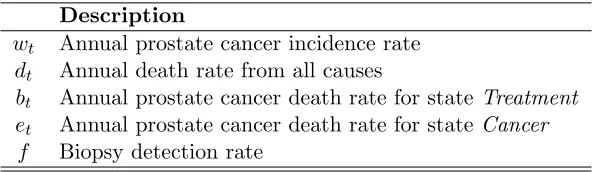
were derived from Surveillance, Epidemiology and End Results (SEER) data and the Mayo Clinic Radical Prostatectomy Registry (MCRPR). Parameters for the transition matrices are defined in Table 4.3.
Description
wt Annual prostate cancer incidence rate
dt Annual death rate from all causes
bt Annual prostate cancer death rate for stateTreatment
et Annual prostate cancer death rate for stateCancer
f Biopsy detection rate
Table 4.1: Parameters for transition probability matrices
Given the decision to biopsy, we define the one-step transition probability matrix as [46]:
NC CND T D
NC P(NC|NC,B) P(CND|NC,B) 0 P(D|NC,B)
CND 0 P(CND|CND,B) P(T|CND,B) P(D|CND,B)
T 0 0 P(T|T,B) P(D|T,B)
D 0 0 0 1
P(NC|NC,B) = (1−dt)(1−wt)
P(CND|NC,B) = (1−dt)wt
P(D|NC,B) = dt
P(CND|CND,B) = (1−f)(1−dt)(1−et)
P(T|CND,B) = f(1−bt)(1−dt)
P(D|CND,B) = f bt(1−dt) +et(1−f)(1−dt)
P(T|T,B) = (1−dt)(1−bt)
P(D|T,B) = dt+bt(1−dt)
In the absence of biopsy (i.e. waiting), we define the one-step transition probability matrix
NC CND T D
NC P(NC|NC,W) P(CND|NC,W) 0 P(D|NC,W)
CND 0 P(CND|CND,W) 0 P(D|CND,W)
T 0 0 P(T|T,W) P(D|T,W)
D 0 0 0 1
P(NC|NC,W) = (1−dt)(1−wt)
P(CND|NC,W) = (1−dt)wt
P(D|NC,W) = dt
P(CND|CND,W) = (1−dt)(1−et)
P(D|CND,W) = dt+et(1−dt)
P(T|T,W) = (1−dt)(1−bt)
P(D|T,W) = dt+bt(1−dt)
After making a core health-state transition, the PSA observation for the next period (if there is another) of the Markov model is observed. The simulation proceeds until the patient transitions to the absorbing state D, i.e., until the patient dies. It is important to note that the Markov chain is partially observable; the core health state is unknown to the observer, but the likelihood of cancer can be inferred from the PSA observation.
The information matrix,Q, is
Q=
0.488 0.318 0.099 0.058 0.017 0.020 0 0 0.253 0.242 0.135 0.170 0.082 0.118 0 0
0 0 0 0 0 0 1 0
0 0 0 0 0 0 0 1
where the rows correspond to core health-states no cancer, cancer, treatment, and death, respectively; and the columns correspond to PSA intervals [0, 1), [1, 2.5), [2.5, 4), [4, 7), [7, 10), [10, ∞), treatment, and death, respectively [46].
4.4
Computing Platforms
System 1. Dell Linux server with 2 Quad-Core Intel Xeon E5420 2.5GHz CPUs and 16GB shared RAM. Compiler: gcc (GCC) 4.1.2 (64-bit target) by the Free Software Foundation, Inc.
System 2. IBM Blade Center Linux Cluster with 4 Quad-Core AMD Opteron 8374 HE 2.2GHz CPUs and 64 GB shared RAM per blade. Compiler: pgCC 7.2-2 (32-bit target) by The Portland Group, Inc.
4.5
Numerical Results
4.5.1 Data and Model Parameters
Table 4.5.1 list the values and sources for the reward parameters used in evaluating the proposed screening policies, where λis the discount factor for the reward function, is the annual utility decrement of living in state T,µ is the one-time utility decrement associated with biopsy,δ is the annual utility decrement of living in state C, and f is the biopsy detection rate for patients with prostate cancer. Unless explicitly stated otherwise, all results in this thesis pertain to the set of parameter values in Table 4.5.1.
Parameter Value Source
0.05 Bremner et al. 2007
µ 0.01 Chhatwal et al. 2008
δ 0 Bremner et al. 2007
λ 1 Gold et al. 1996
f 0.8 Haas et al. 2007
Table 4.2: Reward parameters used in evaluating proposed screening policies
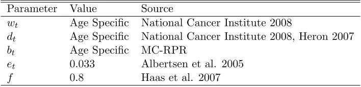
Table 4.5.1 list the values and sources for the state transition probabilities used in evaluating the proposed screening policies, where wtis the annual prostate cancer incidence rate, dt is the
annual death rate from other causes, bt is the annual prostate cancer death rate for patients in
state T, et is the annual prostate cancer death rate for patients in state C, andf is the biopsy
detection rate for patients with prostate cancer. For Table 4.5.1, note that MC-RPR stands for the Mayo Clinic Radical Prostatectomy Registry.
4.5.2 Discounting QALYs
Parameter Value Source
wt Age Specific National Cancer Institute 2008
dt Age Specific National Cancer Institute 2008, Heron 2007
bt Age Specific MC-RPR
et 0.033 Albertsen et al. 2005
f 0.8 Haas et al. 2007
Table 4.3: Transition probabilities used in evaluating proposed screening policies
is controversial, and has a significant effect on optimal policies when rewards are discounted over large time intervals (e.g. decades of a patient’s life). Therefore, we let λ= 1 in order to better distinguish the policies, as illustrated in Figure 4.5.2. Although Figure 4.5.2 appears to graph 6 different functions, it actually graphs 18 different functions; each line is formed by the combination of 3 different lines, whereµ= 0.01, 0.05, and 0.1. At this level of magnification, functions differing only byµ values in the range [0.01,0.1] overlap and are indistinguishable.
A B C D E F G H
16 18 20 22 24 26 28 30
Ross policy
Expected QALY
Sensitivity Analysis on λ and ε
ε=0.05
ε=0.05
ε=0.145
ε=0.24
ε=0.24
ε=0.145 λ=1
λ=0.9924
Figure 4.4: Sensitivity analysis on parameters of reward function for Ross policies
4.5.3 Evaluation of Proposed Screening Policies
the outcome measure quality-adjusted life years (QALYs). These policies (hereafter referred to as the Ross policies) are defined as follows: (A) no screening; (B) threshold 4.0 ng/mL tested every 5 years from age 40 to 75; (C) threshold 4.0 ng/mL tested every 2 years from age 50 to 75; (D) annual testing with threshold 3.5 ng/mL from age 50 to 59, 4.5 ng/mL from age 60 to 69, and 6.5 ng/mL from age 70 to 75; (E) threshold 4.0 ng/mL tested annually from age 50 to 75; (F) threshold 2.5 ng/mL tested annually from age 50 to 75; (G) threshold 4.0 ng/mL tested at age 40, age 45, and every 2 years from age 50 to 75; and (H) threshold 4.0 ng/mL tested at age 40, age 45, and annually from age 50 to 75.
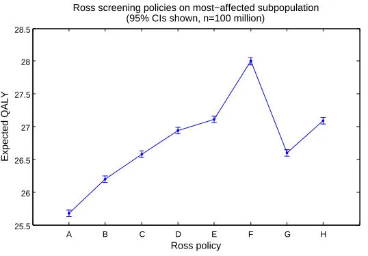
In Figures 4.5.3 and 4.5.3, we examine the effect of the PSA screening policies from Ross (2007) in terms of QALYs. Figure 4.5.3 illustrates results for the entire US male population, whereas Figure 4.5.3 only treats the subpopulation of males who ultimately develop cancer between the ages 50 and 75. It is clear from visual inspection that the range of expected QALYs in Figure 4.5.3 is small. This finding is central to the debate on the benefits of PSA screening. However, the range of expected QALYs in Figure 4.5.3 is much larger. Thus, the policies are significantly different from the perspective of their impact on the most-affected subpopulation. Figure 4.5.3 shows the importance of relying on the most-affected subpopulation — as opposed to the entire US male population — to evaluate a policy on the basis of QALYs.
A B C D E F G H
37.7 37.71 37.72 37.73 37.74 37.75 37.76 37.77
Ross screening policies on entire U.S. male population (95% CIs shown, n=100 million)
Ross policy
Expected QALY
A B C D E F G H 25.5
26 26.5 27 27.5 28 28.5
Ross screening policies on most−affected subpopulation (95% CIs shown, n=100 million)
Ross policy
Expected QALY
Figure 4.6: Ross results comparison for subpopulation of U.S. males who ultimately develop prostate cancer
A B C D E F G H
24 26 28 30 32 34 36 38 40
Comparison between effect on entire U.S. male population and most−affected subpopulation
(95% CIs shown, n=100000000)
Ross policy
Expected QALY
Entire U.S. male population Most−affected subpopulation
4.6
Conclusions
We provide to our knowledge the first results comparing PSA threshold policies based on QALYs. The results from simulating the Ross policies reveal that the best screening policy from the perspective of the general male population is to screen annually from the age of 50 to 75 years with a threshold of 4.0 ng/mL. This policy is the traditional guidelines for PSA-threshold screening currently in practice in the U.S.. Therefore, according to the metric QALYs, and with respect to the entire population of U.S. males, the current PSA screening policy in practice in the U.S. is better than the other Ross policies, such as a common European practice of annual screening from the age of 50 to 75 years with a threshold of 2.5 ng/mL. From a practical standpoint, however, the difference between Ross policies E and F (i.e. between the 4.0 or 2.5 ng/mL thresholds) may be deemed negligible by some.
There are, of course, limitations in our model. Several model parameters are estimates (e.g.
CHAPTER
5
Optimization of PSA-Threshold Screening Policies
In this chapter we discuss our simulation-optimization model and solution method for prostate cancer screening. The optimization problem is to find the set of PSA thresholds as a function of age that maximizes the expected QALYs over a patient’s lifetime.
Our genetic algorithm (GA) explores the space of possible screening policies and evaluates each screening policy by simulation at a specified degree of precision. The greater the portion of the policy space explored by the GA, ceteris paribus, the better the GA. The greater the emphasis on highly fit individuals,ceteris paribus, the better the GA. By increasing exploration, we have a higher probability of reaching the global optimum. By increasing exploitation, we have a higher probability of increasing fitness from generation to generation. Unfortunately, these two attributes—the ability to search a large portion of the policy space (exploration) and the emphasis on promoting higher fitness individuals (exploitation)—are competing; to increase one, is to decrease the other. Therefore, a fundamental consideration in implementing our GA is to find an optimal balance between exploration and exploitation.
Researchers have proposed various strategies for achieving the optimal balance [45],[3], and [35]. Finding the optimal balance between the creation of diversity and the reduction of diversity in favor of exploiting higher fitness individuals is critical to the successful performance of any GA [5]. For more on the tradeoff between exploration and exploitation, see Goldberg [20] or Spears [42].
variants converge as well as how rapidly the variants reach convergence. We experiment with the ranking and selection to devote just enough computational effort to acheive the desired level of exploitation. Chromosomes are evaluated simultaneously on multiple processing cores to make efficient use of computing time.
The remainder of this chapter is structured as follows. After formally defining the optimization problem, we discuss how the ranking and selection procedure gives us a statistical guarantee that the GA will tend toward fitter policies, and how our ranking and selection procedure in concert with parallel processing lightens the computational burden. We then describe in detail the GA and present psuedo-code that may be adapted to other disease treatment/screening optimization problems. Next, we present sensitivity analysis on characteristics of the GA itself (e.g. mutation rate, crossover method). Finally, we present sensitivity analysis on prostate cancer screening policies with respect to parameters of the reward function and transition probabilities.
5.1
Optimization Model
For the PSA screening optimization problem, we seek a PSA screening policy represented by the vector of decision variables,D∗, such that
D∗= arg max
D∈DJ(D), (5.1)
where
J(D) =ED
" T
X
t=t0
λtr(s, a)
#
is the objective function measuring expected QALYs as presented in Chapter 4;D =< d1×
d2× · · · ×dN >wheredi ∈ {0,0.5, . . . ,10,∞}defines the feasible set of PSA-threshold screening
policies; λ is the discount factor over time t; t0 is a lower bound on the age at which PSA
screening begins; T is an upper bound on the age at which PSA screening is discontinued; and
r(s, a) is the reward function as a function of the health state and action.
The optimization problem is difficult because of the combinatorially large number of possible PSA-threshold screening policies and the lack of exploitable mathematical properties (e.g. convexity). Given the limitation of discrete PSA thresholds as defined in the previous paragraph, and assumingt0 = 160 (40 years), there are 22240= 1.5×10322 possible policies. Each policy
5.2
Genetic Algorithm
Genetic algorithms (GAs) search the space of feasible screening policies and evaluate the fitness of the screening policies by simulation. In our simulation-optimization approach, the simulator is embedded in the GA and serves to provide statistical estimates of the expected value of any candidate optimal policy. A high-level model of the algorithm is shown in Figure 5.2.
If stopping criteria is met
Terminate Algorithm Generate
Initial Population
Simulate Population
Reproduction and Mutation
Figure 5.1: High-level model of GA
We use ranking and selection to determine the appropriate sample size for simulating individuals in the population. This provides a statistical guarantee on the probability of correct selection,P(CS). In particular, we use the Rinott procedure. Rinott (1978) presents a now commonly-used two-stage procedure to select the single best of several alternatives [38]. The Rinott procedure is suited to our algorithm because it selects the single best individual (chromosome) from the population that is to be passed along unmodified to the next generation
in keeping with the concept of elitism; a similar strategy is discussed in [7].
The Rinott procedure is based on the least favorable condition, where the best individual differs from the remaining individuals by the indifference amount, δ∗, and the remaining individuals each differ one-to-another by less than the indifference amount. The indifference amount, which is highly problem specific, is the amount greater than or equal to which two individuals must differ in order to be regarded as significantly different. In mathematical terms, the least favorable condition is an arrangement of each individual, Di, such that J(Di) =
J(D∗)−δ∗ for all Di6=D∗. Because the procedure is based on this least favorable condition
used are defined in the following integral equation: Z ∞ 0 " Z ∞ 0 Φ h
{(N0−1) [(1/x) + (1/y)]}1/2
!
f(x)dx
#k−1
f(y)dy=P∗, (5.2)
whereP∗ is a lower bound on the probability of correct selection,N0 is the stage-one sample
size for variance estimation, k is the total number of independent normal individuals in the population, x and y are independent Chi-squared random variables with N0 −1 degrees of
freedom, Φ is the CDF for the standard normal distribution,h is a constant, and f(x) andf(y) are the density functions ofx and y, respectively. The steps of the Rinott procedure are:
1. Simulate each individualDi using sample size N0
2. Simulate each individualDiusing sample sizeNi−N0, whereNi= max (
N0,
h δ∗
2
SD2i )
,
δ∗ is the indifference-zone amount, and SD2
i is the variance of the set ofN0 simulations of Di
3. Compute the expected QALYs for each individualDi, where ¯Xi =
1
Ni
Ni
X
j=1
J(Dij) is the
expected QALYs ofDi, and the random variableX is the simulation performance measure
in QALYs
4. Select as best the individualDi with largest ¯Xi
The basic idea of the Rinott procedure is to provide a guarantee that the single best individual from a population will be selected at least a chosen probability of the time. The procedure allows us to specify a lower-bound on the probability at which we select the best policy from a set of policies. The fundamental information that the procedure provides to us is the sample size that is sufficient and no larger than necessary to guarantee the chosen probability of correct selection.
selection algorithm, which the authors in [48] claim to be the most frequently used selection algorithm. The Roulette Wheel algorithm is a type of fitness-proportional selection method. The probability that a particular chromosome is chosen to be a parent is directly related to the chromosome’s fitness relative to the combined fitness of the entire population.
Each chromosome,k, is ordered by and assigned to a section of the wheel proportional to the chromosome’s fitness (see Figure 5.2). A random number uniformly distributed on the interval [0,1] is generated. The value of the random number will fall into a section of the wheel. The chromosome into whose section of the wheel the random number falls, is the chromosome selected with replacement for reproduction. This selection process repeats until enough chromosomes are selected to produce the required offspring. The offspring will tend to have relatively high fitness values, and, therefore, the offspring is biased towards better prostate-cancer screening policies.
1
0.06
0.19
0.60
0.30 0
k1
k4
k3 k2 k5
Figure 5.2: Example roulette wheel illustration
chromosome with greater fitness is selected with probability 1.
The selection method describes the process by which a chromosome is selected to have its genetic material promoted to subsequent generations. Specifically, the selection method is used to determine parents for the reproduction (crossover) stage. We examine the performance of the GA under the two selection methods, the Roulette Wheel method, and the Tournament method.
The process of mating two parent chromosomes to produce a new child chromosome is accomplished by crossover. The idea behind crossover is to form a new chromosome that shares features of two existing chromosomes. In our problem, the two parents are defined by the following vectors of decision variables:
DP1 = (l1, l2, . . . , lN)
DP2 = (r1, r2, . . . , rN).
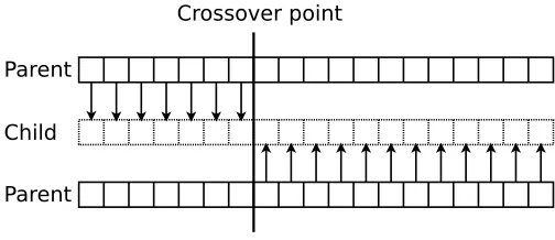
We compare three different crossover methods. The first is called Single-Point crossover [44], and is illustrated by Figure 5.2. This algorithm randomly selects a location q, where
q∈Z: 0< q < N. The vector of decision variables of the resulting child,DC, acquires the first
q decision variables from the first parent, DP1, and the remaining N−q decision variables from
the second parent,DP2, so that the child, after crossover, is defined as
DC = (l0, . . . , lq−1, rq, . . . , rN).
The second crossover method is called Two-Point crossover [44], and is illustrated by Figure 5.2. This algorithm randomly selects two locations pandq. First,p is randomly selected such thatp ∈Z: 0< p < N −1. Then, q is randomly selected such that q ∈Z:p < q < N.
The vector decision variable of the resulting child,DC, acquires the first 0. . . pdecision variables
from the first parent, DP1, the middlep+ 1. . . qdecision variables from the second parent,DP2,
and the last q+ 1. . . N decision variables from the first parent, DP1. The resulting child is,
therefore, defined as
DC = (l0, . . . , lp, rp+1, . . . , rq, lq+1, . . . , lN).
The third crossover method is called Arithmetic crossover [25]. This algorithm simply takes the means (rounded to nearest integers) of the decision variables of both parents,DP1 andDP2,
as the decision variables of the child,DC. The resulting child is, therefore, defined as
DC = (F(l0, r0), . . . ,F(lN, rN)),
where the function F(a, b) returns the rounded average ofaand b.
Crossover point
Parent
Child
Parent
Figure 5.3: Single-point crossover illustration
Crossover points
Parent
Child
Parent
Figure 5.4: Two-point crossover illustration
inheritance of traits that occurs when two species reproduce in nature. The product of this reproduction (i.e. the child) is a combination of the genetic material of the parents. In this way, the hope is to pass good genetic material from two individuals onto a new individual which will replace a less fit member of the population. After time, good genes are promoted over bad genes, and the fitter genetic material survives with greater likelihood.
The crossover method defines the mechanism by which the genetic material of two chromo-somes are combined in order to create a new chromosome; in other words, crossover defines the mechanics of reproduction. We examine the performance of the GA under each of the 3 crossover methods implemented.
The mutation rate is the probability that a gene (i.e. decision variable) will be mutated (i.e. randomly changed). The mutation rate is equal for every gene. The goal in selecting a mutation rate is to choose the rate which satisfactorily promotes diversity without disturbing substrings that positively contribute to the fitness of the chromosomes. From Figure 5.3.1, we conclude that the mutation rate 0.001 is appropriate for our GA; accordingly, the mutation rate 0.001 is often recommended in the literature [44].
optimally, the GA provides a lower bound on the maximum expected QALYs that can be achieved through PSA-threshold based prostate cancer screening. Psuedo-code for the genetic algorithm is shown in Algorithm 1; the genetic algorithm’s sub-routines are shown in Algorithms 2, 3, and 4.
Algorithm 1: GeneticAlgorithm()
begin
1
Generate initial population of policies;
2
whilestopping criteria not met do
3
foreachpolicy Di do 4
Use Rinott method to determine sample size,Ni, for desiredP∗; 5
Simulate policy using determined sample size;
6
Record J(Di); 7
BestPolicy ← policy with greatest expected QALYs;
8
Jmax←J(BestPolicy);
9
foreachpolicy Di do 10
if J(Di)6=Jmax then 11
Parent1 ← TournamentSelect();
12
Parent2 ← TournamentSelect();
13
NewPolicy← Crossover(Parent1,Parent2);
14
Mutate(NewPolicy);
15
Di← NewPolicy;
16
returnBestPolicy;
17
end
18
Algorithm 2: TournamentSelect() Output: Selected policy
begin
1
DA← randomly selected policy from entire population of policies; 2
DB ←randomly selected policy from entire population of policies; 3
if J(DA)> J(DB) then 4
returnDA; 5
else
6
returnDB; 7
end
Algorithm 3: Crossover(Parent1, Parent2)
Input: Parent policies which reproduce to form a new policy Output: New policy formed by reproduction
begin
1
cxpoint1 ← random integer∈[1,400−1];
2
cxpoint2 ← random integer∈[cxpoint1 + 1,400];
3
fori = 1 to cxpoint1 do
4
NewPolicy[i]← Parent1[i];
5
fori = cxpoint1+1 to cxpoint2 do
6
NewPolicy[i]← Parent2[i];
7
fori=cxpoint2+1 to 400do
8
NewPolicy[i]← Parent1[i];
9
returnNewPolicy;
10
end
11
Algorithm 4: Mutate(Policy) Input: Policy to be mutated Output: Mutated policy begin
1
fori=1 to 400 do
2
x←uniform random variate ∈[0,1];
3
if x≤0.001then
4
Policy[i] ← randomly selected PSA threshold∈ {0,0.5, . . . ,10,∞};
5
returnPolicy;
6
end
5.3
Results
The following subsections contain sensitivity analysis on running time of the simulator (objective function estimator), sensitivity analysis on parameters of the reward function, sensitivity analysis on parameters of the GA, and numerical analysis of the optimal policy produced by the GA.
5.3.1 Experimental Evaluation of Genetic Algorithm
Table 5.3.1 provides results from single simulations run on a single threshold and screening frequency policy, where random variates in the stochastic model were drawn from the same random number stream. These results show the effect of sample size and point out the tradeoff between precision of our expected QALY calculation at the 95% confidence level and the compute time required to make such calculation. The relative precision is the confidence interval half-length divided by the midpoint of the confidence interval; this measure expresses the margin for error as a fraction of the estimated quantity (i.e. expected QALYs).
# Sample size Half width (QALY) Relative precision Run time (sec)
1 1,000 22.615 94.58% 0.02
2 10,000 4.972 16.28% 0.24
3 100,000 1.530 5.65% 2.38
4 200,000 1.091 4.06% 4.77
5 300,000 0.873 3.32% 7.15
6 400,000 0.754 2.87% 9.53
7 500,000 0.671 2.56% 11.90
8 600,000 0.615 2.35% 14.29
9 700,000 0.566 2.16% 16.67
10 800,000 0.525 2.01% 19.06
11 900,000 0.495 1.89% 21.42
12 1,000,000 0.471 1.80% 23.81
13 10,000,000 0.151 0.57% 238.13
14 100,000,000 0.048 0.18% 2392.50
Table 5.1: Precision and running time analysis
them and produce better offspring, all that is needed is a reliable measure to determine the optimality of the populations relative to each other. At this stage, we do not need to estimate the actual optimal value of the populations; a simple ordering is sufficient. Since smaller sample sizes require less compute-time, selecting a sample size which is no more precise than necessary allows the metaheuristic to search a larger solution space in a given period of time.
It is notable that a very large number of samples is required to achieve high precision. This is consistent with findings in the medical literature that demonstrate difficulty in differentiating screening policies through randomized controlled trials. This also motivates the need to carefully consider computational effort and the tradeoff between exploration and exploitation, as in our proposed simulation-optimization method.
1e3 1e5 3e5 5e5 7e5 9e5 10e7 23
24 25 26 27 28 29 30 31
Sample Size
Expected QALY
Convergence of Mean
Figure 5.5: Convergence of mean as sample size increases
The performance of the single-point, two-point, and arithmetic crossover methods are shown below, respectively, in Figure 5.3.1. Although the single-point method and the two-point method achieve roughly the same level of fitness at the end of 500 generations, the two-point crossover method shows slightly more rapid convergence. For this reason, we prefer the two-point method over the single-point method. By inspection it is clear that the arithmetic method performs poorly in comparison to the single-point and the two-point methods. On the basis of this analysis, we conclude that the two-point crossover method is superior for our particular problem.
0 100 200 300 400 500 37.7 37.72 37.74 37.76 37.78 37.8 37.82 Single−Point crossover Generation Expected QALY
0 100 200 300 400 500 37.7 37.72 37.74 37.76 37.78 37.8 37.82 Two−Point crossover Generation Expected QALY
0 100 200 300 400 500 37.7 37.72 37.74 37.76 37.78 37.8 37.82 Arithmetic crossover Generation Expected QALY
Figure 5.6: Comparison of crossover methods
then each chromosome will have nearly equal relative fitness. Because roulette selection uses the relative fitness of each chromosome to determine the probability of the chromosome being selected, each chromosome is nearly equally likely to be selected. Therefore, when there is little difference in fitness between each chromosome, roulette selection is nothing more than uniform random selection. Tournament selection, on the other hand, provides some assurance that more fit chromosomes will be selected over less fit chromosomes. Unlike roulette selection, tournament selection does not regard the magnitude of differences in fitness. In the PSA screening problem, the differences in fitness between chromosomes are slight. Therefore, we should intuitively expect Tournament selection to perform better.
0 100 200 300 400 500 37.7 37.72 37.74 37.76 37.78 37.8 37.82
Roulette Wheel selection
Generation
Expected QALY
0 100 200 300 400 500 37.7 37.72 37.74 37.76 37.78 37.8 37.82 Tournament selection Generation Expected QALY
Figure 5.7: Comparison of selection methods
slope of the fitness function decreases sooner and more rapidly as the mutation rate increases from 0.001. Therefore, we take 0.001 as the mutation rate for the PSA screening problem.
0 100 200 300 400 500 37.7 37.72 37.74 37.76 37.78 37.8 37.82
Mutation rate = 0.001
Generation
Expected QALY
0 100 200 300 400 500 37.7 37.72 37.74 37.76 37.78 37.8 37.82
Mutation rate = 0.002
Generation
Expected QALY
0 100 200 300 400 500 37.7 37.72 37.74 37.76 37.78 37.8 37.82
Mutation rate = 0.003
Generation
Expected QALY
Figure 5.8: Comparison of mutation rates
5.3.2 Experimental Evolution of Genetic Algorithm
Figures 5.3.2 and 5.3.2 display the evolutionary progress (i.e. the results over time) of the GA using two-point crossover, tournament selection, and mutation rate 0.001; only the most fit chromosome at each generation is used in the graphs. It is clear that the fitness progresses over time. At the 95% confidence level, the fitness of the initial population is statistically different from the fitness of the populations beginning around the 200th generation. Therefore, we have statistical confidence that the most-fit policy improves over time.
From Figure 5.3.2 we see that the GA appears to converge to an optimum around the 1,500th generation. Because GAs are heuristic search algorithms, there can be no guarantee derived from the GA itself that the global optimum has been reached; it is always possible to converge to a local optimum. However, we believe a near optimal solution has been reached (we provide justification for this in Section 5.3.5).
5.3.3 Optimal PSA Screening Policies
0 100 200 300 400 500 600 700 800 900 1000 37.72
37.74 37.76 37.78 37.8 37.82
Evolutionary progress of GA (95% CIs shown)
Generation
Expected QALY
Figure 5.9: Evolution of GA showing period of sharpest incline in fitness improvement from generation to generation
0 500 1000 1500 2000 2500 3000 37.72
37.74 37.76 37.78 37.8 37.82 37.84
Evolutionary progress of GA (95% CIs shown)
Generation
Expected QALY
the age 65-70. Once a patient is biopsied, the patient is removed from the model. Therefore, all data after the first 0.0 ng/mL threshold is meaningless, and the 0.0 ng/mL threshold serves the purpose of excluding screening beyond the age 65-70.
40 45 50 55 60 65
0.0 0.5 1.0 1.5 2.0 2.5 3.0 3.5 4.0 4.5 5.0 5.5 6.0 6.5 7.0 7.5 8.0 8.5 9.0 9.5 10.0 infinity
Optimal PSA Screening Policy (raw)
Age (years)
PSA Threshold (ng/mL)
Figure 5.11: Optimal PSA screening policy discovered by GA in raw form
5.3.4 Clinically Relevant Screening Policies
Because of the nature of a GA, the optimal policy discovered by the GA will inevitably exhibit some imperfect or non-smooth patterns. In the context of a clinically implementable screening policy, these imperfectly patterned policies should ideally be simplified to a policy that is reasonable to implement. We consider two simplification methods. First, for the policy shown in Figure 5.3.4, starting from the initial age of screening we accept only those thresholds lying on a non-decreasing curve. That is, for each decision epoch,tn, if the PSA threshold at tn−1 is less
than or equal to the PSA threshold attn, we accept the threshold at tn; otherwise, we discard
the threshold attn. (Note that we also arbitrarily discarded as an anomaly the threshold att0 =
age 40.) Second, for the policy shown in Figure 5.3.6, we arbitrarily accept certain thresholds such that the simplified policy appears more reasonable to implement. This second method does not lend itself to algorithmic description because it is inherently ad hoc and arbitrary.
as good as the raw policy, but more reasonable to implement. Because, in both Figure 5.3.4 and Figure 5.3.6, the 95% confidence intervals for the raw and simplified optimal policies overlap, or nearly overlap, we cannot say that the simplified policies are better or worse than the respective raw policies. By inspection, it is clear that the simplified policies—though not trivial to implement—are indeed more reasonable to implement than the respective raw policies. Having achieved these goals, the simplified policies and the methods of simplification are valid.
40 45 50 55 60 65 70 75 80 85 90 95 100
0.0 0.5 1.0 1.5 2.0 2.5 3.0 3.5 4.0 4.5 5.0 5.5 6.0 6.5 7.0 7.5 8.0 8.5 9.0 9.5 10.0 infinity
Optimal PSA Screening Policy (simplified)
Age (years)
PSA Threshold (ng/mL)
Figure 5.12: Optimal PSA screening policy discovered by GA in simplified form
A B C D E F G H raw simplified 37.7
37.72 37.74 37.76 37.78 37.8 37.82
Simulation comparison of Ross policies to optimal policy from GA (95% CIs, n=100000000)
Policy
Expected QALY
Figure 5.13: Comparing the Ross policies to the optimal GA policy (both the raw version and the simplified version) in terms of the effect on the entire U.S. male population
A B C D E F G H raw simplified
25.5 26 26.5 27 27.5 28 28.5
Simulation comparison on subpopulation of Ross policies to optimal policy from GA
(95% CIs, n=100000000)
Policy
Expected QALY
5.3.5 Upper Bounds on the Optimal Policy
Zhang (2010) formulated a partially-observable Markov decision process (POMDP) to determine the theoretical optimal PSA-threshold screening policy using the same original data set that we used. The POMDP uses Bayesian updating to use all prior PSA tests to estimate the patient’s probability of having prostate cancer. This probability is then used to decide whether to refer the patient for biopsy and subsequent treatment. This is markedly different from our GA, which specifies according to age the PSA threshold at which to biopsy based on a single independent PSA observation.
In Table 5.2, we compare the benefits of the optimal policy found using the POMDP in Zhang (2010) with the benefits of the near optimal policy found using our genetic algorithm (shown in Figure 5.3.4). The POMDP model and the best GA policy found for comparison to the POMDP model, use parameter values = 0.145 andµ= 0.05; the other parameter values are as previously defined in Table 4.5.1. Because the POMDP provides theoretical upper bounds on the optimal policy, it is expected that the best GA policy is less effective. However, it is worth noting that PSA-based thresholds are the norm in clinical practice. Whereas the POMDP solution provides insights into the theoretical maximum benefit in QALYs of PSA screening, the GA provides insights into how close we may come in practice to the theoretical maximum benefit.
Per person expected Per person expected improvement (in QALYs) improvement (in QALYs)
over no screening over traditional guidelines
GA 0.008 0.022
POMDP 0.033 0.060
Table 5.2: Comparison between the best GA policy and the optimal POMDP policy [47]
5.3.6 Multiple Biopsy
The assumption that every patient may undergo at most one biopsy during his lifetime is reasonable. In our dataset 81.4% of patients biopsied underwent only 1 biopsy. However, it is worthwhile to investigate the best GA policy under the assumption that every patient may undergo at most three biopsies. The limit of 3 biopsies is supported by anecdotal clinical evidence.
assumption that every patient may undergo up to three biopsies. Figures 5.3.6 and 5.3.6 show the best policy found by the GA under the three biopsy assumption in raw and simplified form, respectively.
40 45 50 55 60 65 70 75 80
0.0 0.5 1.0 1.5 2.0 2.5 3.0 3.5 4.0 4.5 5.0 5.5 6.0 6.5 7.0 7.5 8.0 8.5 9.0 9.5 10.0 infinity
Optimal PSA Screening Policy (raw)
Age (years)
PSA Threshold (ng/mL)
40 45 50 55 60 65 70 75 80 85 90 95 100 0.0
0.5 1.0 1.5 2.0 2.5 3.0 3.5 4.0 4.5 5.0 5.5 6.0 6.5 7.0 7.5 8.0 8.5 9.0 9.5 10.0 infinity
Optimal PSA Screening Policy (simplified)
Age (years)
PSA Threshold (ng/mL)
Judging from Figure 5.3.6, it is clear that the best policy performs better than the Ross policies from the perspective of the entire US male population. Judging from Figure 5.3.6, however, the best policy isnot optimal with respect to the subpopulation of males who ultimately develop cancer. The improvement in Figure 5.3.6 is greater than the loss in Figure 5.3.6. And the optimal policy in Figure 5.3.6 is on par with most of the Ross policies. For these reasons, we believe the best policy generated by the GA to be the overall optimal PSA screening policy.
A B C D E F G H raw simplified
37.7 37.75 37.8 37.85
Simulation comparison of Ross policies to optimal policy from GA (95% CIs, n=1000000)
Policy
Expected QALY
A B C D E F G H raw simplified 25.5
26 26.5 27 27.5 28 28.5
Simulation comparison on subpopulation of Ross policies to optimal policy from GA
(95% CIs, n=100000000)
Policy
Expected QALY
5.3.7 Sensitivity Analysis
We now present sensitivity analysis from the prostate-cancer screening perspective. Table 5.3.7 presents sensitivity analysis data concerned with the effect of the best GA policy on the entire U.S. male population. Table 5.3.7 presents sensitivity analysis data concerned with the effect of the best GA policy on the subpopulation of U.S. males who ultimately develop prostate cancer. While we examine the effects on two different populations, the optimal policy is optimal because of its effect on one single population, the entire U.S. male population.
It is clear from Tables 5.3.7 and 5.3.7 that the discount factor, λ, is the most influential parameter. In Table 5.3.7 we see that the best GA policy always outperforms the traditional U.S. policy, in terms of the effect of screening on the entire population, but the best GA policy is better than no screening for only roughly half of the parameter values.
λ µ Expected QALYs Improvement over Improvement over
under best GA policy no-screening (%) US policy (%)
0.9924
0.05
0.01 21.580 0.042 0.009
0.05 21.555 0.074 0.019
0.1 21.569 -0.009 0.246
0.145
0.01 21.568 -0.014 0.000
0.05 21.558 -0.060 0.079
0.1 21.570 -0.005 0.293
0.24
0.01 21.560 -0.051 0.005
0.05 21.561 -0.046 0.135
0.1 21.571 0.000 0.344
1
0.05
0.01 37.778 0.186 0.077
0.05 37.750 0.111 0.074
0.1 37.713 0.013 0.069
0.145
0.01 37.732 0.064 0.029
0.05 37.706 -0.005 0.032
0.1 37.708 0.000 0.130
0.24
0.01 37.706 -0.005 0.034
0.05 37.708 0.000 0.112
0.1 37.708 0.000 0.205
λ µ Expected QALYs Improvement over Improvement over
under optimal policy no-screening (%) US policy (%)
0.9924
0.05
0.01 17.198 3.06 0.29
0.05 16.925 1.42 -1.20
0.1 16.707 0.11 -2.34
0.145
0.01 17.038 2.10 0.87
0.05 16.720 0.19 -0.91
0.1 16.687 -0.01 -0.97
0.24
0.01 16.664 -0.14 0.19
0.05 16.664 -0.14 0.29
0.1 16.688 0.00 0.57
1
0.05
0.01 26.640 3.63 -1.70
0.05 26.465 2.95 -2.28
0.1 26.250 2.11 -2.99
0.145
0.01 26.472 0.33 -2.47
0.05 25.793 0.33 -2.47
0.1 25.707 0.00 -2.71
0.24
0.01 25.809 0.40 -0.06
0.05 25.707 0.00 -0.39
0.1 25.707 0.00 -0.30