Bayesian Mapping of Multiple Quantitative Trait Loci From Incomplete Inbred Line Cross Data

Copyright1998 by the Genetics Society of America

Bayesian Mapping of Multiple Quantitative Trait Loci From

Incomplete Inbred Line Cross Data

Mikko J. Sillanpa¨a¨ and Elja Arjas

Rolf Nevanlinna Institute, University of Helsinki, FIN-00014 Finland

Manuscript received April 7, 1997 Accepted for publication November 17, 1997

ABSTRACT

A novel fine structure mapping method for quantitative traits is presented. It is based on Bayesian modeling and inference, treating the number of quantitative trait loci (QTLs) as an unobserved random variable and using ideas similar to composite interval mapping to account for the effects of QTLs in other chromosomes. The method is introduced for inbred lines and it can be applied also in situations involving frequent missing genotypes. We propose that two new probabilistic measures be used to summarize the results from the statistical analysis: (1) the (posterior) QTL-intensity, for estimating the number of QTLs in a chromosome and for localizing them into some particular chromosomal regions, and (2) the locationwise (posterior) distributions of the phenotypic effects of the QTLs. Both these measures will be viewed as functions of the putative QTL locus, over the marker range in the linkage group. The method is tested and compared with standard interval and composite interval mapping techniques by using simulated backcross progeny data. It is implemented as a software package. Its initial version is freely available for

research purposes under the name Multimapper at URL http://www.rni.helsinki.fi/zmjs.

W

cally divergent lines are crossed, all offspring (F1 andBotstein1989), least squares method (Haleyand

generation) are genetically identical, being heterozy- Knott1992), and composite interval mapping (Jansen

gous at each locus. In the haplotypes of the F1individu- 1993;Jansen and Stam 1994; Zeng 1993, 1994). For

als, the locus next to each quantitative trait locus (QTL) some species, it is very impractical, time consuming and

has the same allele as it had in the parental haplotype. also expensive to produce inbred lines. In such cases,

This is because, in this ideal case, parents are homozy- methods have been developed for considering crosses

gous at each locus and recombination events cannot between outbred lines that are genetically divergent and

change haplotypic arrangements. Therefore, linkage show two very separate groups of phenotypic values, for

disequilibrium (nonrandom allelic association) in this _{example, due to different selection histories. One such}

group is maximal. _{procedure was presented in}Haleyet al. (1994), where

When an F2or backcross generation is produced, link- the analysis was done in terms of line origins, with the

age disequilibrium is reduced slightly but still remains _{assumption that crossed lines are “fixed” for different}

at a high level. The degree of reduction depends on _{genes (or alleles) and would then show homozygosity}

the distance and on the recombination fraction between _{in most of the QTL loci. This method (design) requires}

the considered QTL and the nearby marker locus. If _{genotypic data from the parental and grandparental}

mating is continued till F3and the succeeding genera- _{generations in addition to genotypic and phenotypic}

tions, disequilibrium area surrounding a QTL is re- _{offspring data. Recently} Jansen (1996) introduced a

duced further in each generation. This is why the back- _{general method for line crosses by applying the}

EM-cross or F2 intercross data from inbred lines is _{algorithm (}Dempsteret al. 1977), where the evaluation

particularly suitable for QTL mapping. _{of the expectation step was conducted by a Markov chain}

The commonly used QTL mapping methods for _{Monte Carlo (MCMC) technique analogous to that of}

plants and animals introduced recently use offspring Guo and Thompson (1992). All these methods are

data from divergent inbred lines in backcross or F2in- _{based on the assumption that the distribution of the}

tercross design. The reason for using such a design is _{phenotypes is Gaussian. A robust method in this respect}

to maximize linkage disequilibrium and the amount of _{was developed recently by} Kruglyak and Lander

heterozygosity (information content) in meioses. Exam- _{(1995). Modifications of (composite) interval mapping}

to binary traits were presented byVisscheret al. (1996a)

and Xu and Atchley (1996), and a QTL mapping

Corresponding author: Mikko J. Sillanpa¨a¨, Rolf Nevanlinna Institute, _{method for ordinal categorical traits by}Hackett and

Research Institute of Mathematics, Statistics, and Computer Science,

Weller(1995).

P.O. Box 4, FIN-00014 University of Helsinki, Finland.

E-mail: [email protected] In interval mapping (Lander and Botstein 1989),

which is currently used routinely for QTL mapping of the number of influential QTLs as well as estimating their locations in the (analyzed) chromosome and the

(Mapmaker/QTL byLincolnet al. 1992), it is possible

to calculate likelihood scores for a putative QTL placed corresponding phenotypic effects. Such a possibility was

hinted at in a conference presentation by A. F. M. in any position between two adjacent flanking markers.

By changing the flanking markers one at a time, it is Smith(1996), and it has been explicitly implemented

by Satagopan and Yandell (1996), Stephens and

possible to determine the likelihood curve over the

whole genome. The procedure is based on regression Fisch(1996), and UimariandHoeschele(1997).

MCMC methods (Metropoliset al. 1953;Hastings

of phenotypes on QTL genotypes, and because QTL

genotypes are unknown, results are obtained by using 1970) are not new techniques, but their widespread

application in statistics did not start before the introduc-an iterative EM algorithm in which convergence to a

local maximum is guaranteed. For each fixed location tion of Gibbs sampling (GemanandGeman1984). For

a review of applications in gene mapping seeThompson

separately, the algorithm searches the parameter vector

value giving the highest likelihood score. These (profile (1994), Thomas and Gauderman (1995) and

refer-ences therein. An excellent introduction to the Gibbs likelihood) scores are then used to draw the LOD-score

curve corresponding to different QTL positions. sampling and to the Metropolis-Hastings (M-H)

algo-rithm can be found fromCasellaandGeorge(1992),

The composite interval mapping procedure

intro-duced by Zeng (1993, 1994), and the multiple-QTL andChib andGreenberg(1995). More advanced

pa-pers areGeyer(1992), andBesaget al. (1995). Variable

mapping of Jansen (1993) and Jansen and Stam

(1994), are in principle similar to interval mapping ex- dimensional parameterizations are considered inArjas

andGasbarra(1994), and Green(1995).

cept that also some markers outside the tested interval

(also in other chromosomes) are fitted to the model as Bayesian inference for gene mapping has been

consid-ered by Tai (1989), Thomas and Cortessis (1992),

covariates in order to reduce background noise caused

by other QTLs and/or polygenic variation. The most SmithandRoberts(1993), andStephensandSmith

(1993). A Bayesian QTL mapping method was proposed significant markers for such reduction can be chosen

in a preliminary analysis by using stepwise regres- recently bySatagopanet al. (1996), where a

prespeci-fied number of QTLs was assumed to be present in the sion. These background control markers lie near the

QTLs and they are used instead of the true QTLs (whose considered chromosome. The method did not take into

account effects of QTLs in other chromosomes. Judge-locations are unknown), yielding a better resolution

than would be possible if those QTL effects were not ment concerning the actual numbers of QTLs (in the

model) was proposed to be made by using Bayes factors considered at all. Theoretical support is provided by

the fact that when a QTL has an effect on the trait one from separate MCMC runs with different numbers of

QTLs in each. Satagopan and Yandell (1996), and

can see the same effect indirectly through the closest

marker which is in linkage disequilibrium with the QTL Stephens and Fisch (1996) considered all

chromo-somes simultaneously, treating the number of QTLs as (Tanksley1993). The degree by which the

correspond-ing phenotypic effect is reduced is determined by the a random variable. [The example in Satagopanand

Yandell(1996) included only one chromosome,

how-recombination fraction between the marker and the

QTL. However, there should be at least some effect, ever.] Satagopan and Yandell (1996) used an M-H

within Gibbs scheme in estimation, in contrast to an M-H because linkage disequilibrium is almost at its maximum

value in the backcross and F2intercross population. The scheme applied byStephensandFisch(1996), as well

as here.StephensandFisch(1996) simulated 10

chro-improvement in resolution of the composite interval

mapping over standard interval mapping is sometimes mosomes in 6 different datasets, with a different

herita-bility in each. They also tested several priors. However,

huge (e.g.,Kuittinen et al. 1997), thus yielding more

putative QTL findings. However, the method does not they did not consider missing data.

Bayesian QTL mapping in outbred livestock popula-yet seem to be widely used in practice, even though it

is implemented in some software packages (e.g., QTL tion, using granddaughter design, has been studied by

Uimari et al. (1996a,b) and Uimari and Hoeschele

Cartografer byBastenet al. 1996, and MapQTL byvan

OoijenandMaliepaard1996, and PLABQTL byUtz (1997). A Gibbs sampler was used in single and bi-QTL

models which included both major gene and polygenic

andMelchinger1996).

The purpose of this paper is to present an approach effects. UimariandHoeschele(1997) also tested the

idea of a variable dimensional model, considering for high resolution QTL mapping in inbred line crosses

from incomplete data when the phenotypic distribution the cases of either zero, one or two QTLs and using the

convention that the second QTL, if present, was always is assumed to be Normal. Our modeling approach is

based on regression and the assumption that individual “to the right” of the first one. They concluded that their

method was sensitive to the way in which the parameters QTL effects are additive. The method belongs to the

general framework of variable dimensional Bayesian of the second QTL were chosen. Effects of major QTLs

in the other chromosomes were not taken into account

models (e.g.,Green1995), applying MCMC algorithms

related techniques in multi-generational pedigrees are types at any (marker or QTL) locus, ordered so that all

difficult to apply. Apart from Uimari et al. (1996a), _{homozygote genotypes come before heterozygotes. In}

techniques for handling missing genotypic data were this setting, genotypes AB and BA are considered to be

not considered. the same. The regression parameters are the following:

The contents of this paper are as follows. Next, we a is the regression intercept (mean value), bq5(bq1, ...,

describe our statistical model. The results from simula- bqNgen) is a vector of regression coefficients (classification

tion experiments are described thereafter. The final _{variables) where bq jis the regression coefficient for the}

section contains a discussion of the method and of the _{qth QTL genotypeaj at location lq,s}25 _Var(e

i) is the

experiences we had. In appendix a we outline the _{residual variance and C} 5 _(c

kj) is an Nbc 3 Ngen matrix

MCMC algorithm used in the estimation. _{of regression coefficients ckj for background controls.}

We consider the following statistical model for y:

MODEL _y

i 5a 1

o

q51

o

j51

bq j1{x qi5aj } 1

o

k51

o

j51

ckj1{X *ik5aj}1ei. (1)

QTL search is usually concentrated on a given

chro-Here 1{x_qi5aj} is the indicator variable (dummy), which

mosome (or chromosomal segment). Therefore

every-thing in the following is with respect to such a chosen takes value one if the ith individual’s q th QTL genotype

fixed linkage group (chromosome) unless the contrary xqi at location lq is aj, and otherwise its value is zero.

is stated. Let y 5 (y1,y2, ..., yNind) denote the vector of Similarly, 1{X *ik5aj} is the indicator variable taking value

known phenotypes (missing phenotypes are not consid- _{one if the ith individual’s marker genotype in the kth}

ered here), where Nind is the number of individuals in _{background control is}a

jand otherwise its value is zero.

the experiment and yiis the phenotype of the ith indi- _{Here we assume that the residuals e}

i are independent

vidual. Suppose that the observations yiare distributed _{and normally distributed according to N(0,}s2_{). In order}

according to a normal law resulting from some design _{to maintain the traditional way of considering gene}

ef-in ef-inbred lef-inecross data. We shall view the unknown _{fects one can make the following convention. In the}

number of QTLs, denoted by Nqtl, as an unobserved _{case of three possible genotypes, say}a 5_(AA,BB,AB),

random variable. Denote the QTL locations by l5(l1,l2, _{the constraint bq2}5 2_{bq1will produce an additive effect}

..., lNqtl) and letxbe an Nqtl3Nindmatrix, where the qth _{for homozygotes and make b}

q3 correspond to a

domi-column xq5(xq1,xq2, ...,xqNind)9is the QTL genotype vec- nance effect of a heterozygote for each q. For the

back-tor in location lq, with element xqireferring to the ith ground control parameters, the constraint c_k25 2c_k1for

individual. Let G* and G be the corresponding complete _{k5 1, ..., Nbc will have a similar interpretation. In case}

and incomplete (observed) marker information respec- _{of backcross, the corresponding constraints are bq150}

tively; G* and G are taken to be Nind3N matrices, where and c_k15 0, respectively.

N is the number of markers. Let I be the chromosomal We use the shorthand notationd 5(a,b1, ..., bNqtl,s2,C)

interval with the first and the last markers of the chromo- _{andu 5(d,x,l,G*,X *}

o,Nqtl). Notation A*zA means that

some as endpoints. A fixed marker map (i.e., known _{A* is consistent with A in cases where A is incomplete}

recombination fractions between markers whose order _{(observed) and A* is complete information. From}

is known), denoted by m, is assumed known before the _{Bayes’ theorem, we get p(u|y,G,X}

o,m) 5 1/p(y,G,Xo|m)

analysis. _p(y,u,G,X

o|m), where the joint density p(y,u, G,Xo|m) can

We denote complete and incomplete (observed) _{be factored into a likelihood and a (joint) prior density}

marker information in other chromosomes respectively _{as p(y,u,G,X}

o|m) 5p(y,G,Xo|u,m)p(u|m). Here the

likeli-by G*o and Go. Let X *o be a subset of the complete marker hood can be further written into the form of the product

information in other chromosomes, consisting of se- _p(y,G,X

o|u,m) 5 p(G|u,m)p(Xo|G,u,m)p(y|u,m,G,Xo) 5

lected columns (marker genotype vectors) of G *o. Using _{1{G *zG}1}

{X *ozXo}p(y|u,m). In this, 1{G *zG }and 1{X *ozXo}are

indica-an obvious set notation, X *o ,G *o. Similarly, let Xobe a _{tors taking values one and zero depending on whether}

subset of incomplete marker information, Xo, Go. We _{the complete genotypes G* in the chromosome and in}

assume that X *o is chosen to correspond to known back- _{the background control sites X*}

o (in the other

chromo-ground control information (a selected set of markers _{somes) are consistent with their observed incomplete}

that are hoped to be close to influential QTLs outside _{counterparts or not.}

the interval I ). Again, we arrange X *o into the form of _{As for the joint prior distribution p(}u|_{m), given the}

an Nind3 Nbc matrix and denote its (i,k)th element by _{marker map m, we make the following (conditional)}

X *ik, corresponding to the genotype of the ith individu- _{independence assumptions:}

al’s kth background control. Here, Nbcis the number of

(i) Given Nqtl, the vectordconsisting of the parameters

background controls.

of the linear model (1) is independent of the other In the chosen design (i.e., experimental cross), let

coordinates ofu, i.e., of (x,l,G *,X*o), as well as of m;

Ngenbe the number of possible genotypes and let a 5

control genotypes in other chromosomes, is indepen- where

dent of (x,l,G *,Nqtl), the true marker and

QTL-informa-p(M *s11,i|M *s,i,m)5rs,s111{M*s,i?M*s11,i}1(12rs,s11)1{M*s,i5M*s11,i}

tion in the considered chromosome as well as of the

(6) marker map m;

(iii) the true genotypes at marker locations, G *, are is the probability of having genotype M*s11,iat the marker

conditionally independent of the number of QTLs (Nqtl) position s11 in case there is genotype M*s,iat position

and their locations (l ) given the marker map m. _{s, and p(M *1,i) is the probability of genotype M*1,i at a}

marker locus 1 in individual i. Here rs,s11is the

recombi-Then the joint prior density function can be factored

nation fraction between the markers s and s11. (Note

further and be presented in the product form

that rs,s115rs11,s, and therefore also p (M*s11,i|M *s,i,m)5

p(u|m)5 p(G *|m)p(Nqtl|m)p(l|m,Nqtl) p(M *s,i|M *s11,i,m).)

p(x|G*,l,m,Nqtl)p(d|Nqtl)p(X *o). (2) In the case of F₂ intercross, for each individual the

transition probabilities p(M *s11,i|M *s,i,m) from position s

The density p(X *o) is not conditioned on the fixed

to s11 can be arranged into the 333 matrix containing

marker map, because the prior for genotypes can be

all possible transitions between states AA, BB, and AB thought not to be dependent on the marker order or

distances. The posterior density ofuis then proportional

to the joint density







(12rs,s11)2 r2s,s11 2rs,s11(12rs,s11)

r2

s,s11 (12rs,s11)2 2rs,s11(12rs,s11) rs,s11(12rs,s11) rs,s11(12rs,s11) 122rs,s11(12rs,s11)







p(u|y,G,Xo,m)~p(u|m)p(y,G,Xo|u,m)5

(7)

p(u|m)p(y|u,m)1{G *zG,X *ozXo}, (3)

The prior distribution of Nqtl, the number of QTLs, is

where here assumed to be truncated Poisson, where the

Pois-son meanl and the maximum number Nqtlmaxof QTLs

are fixed control parameters such that 0 # l # Nqtlmax.

p(y|u,m)5

p

N_ind

i51

1

√

3

1 2s2

The upper bound Nqtlmaxis introduced for computational

reasons.

(yi2(a1

o

Nqtl

q51

o

j51

bq j1{x qi5aj }1

o

k51

o

j51

ckj1{x*ik5aj })) 2

4

In the following, we shall use the generic term “ob-ject” for any marker or QTL in the chromosome. The

is the likelihood function (normal density) constructed prior distribution of QTL genotypes at locations l is

from residuals ei. Here complete background control assumed to have the following product form:

genotypes X*ik are determined uniquely from X *o. The

p(x|G*,l,m,Nqtl)5

p

Nqtl

q51

p(xq|G*,x1,.,xq21,l,m)

expression for the posterior distribution depends on the prior densities, where the parameter values are

re-stricted to only that part of the parameter space which ₅

p

q51

p

i51

p(xqi|G*iLq,G*iRq,rq) . (8)

is consistent with what is already observed.

In specifying prior densities it is important to note

Here, G*q

iL and G*iRqare the genotypes of the left and the

that the number of possible alleles and genotypes (Ngen)

right flanking object (marker or QTL) for the qth QTL depends on the (experimental) design in question.

in individual i, chosen among the complete set of the

Therefore, also the prior densities p(x|G *,l,m,Nqtl),

markers in the chromosome and the QTLs at positions

p(G*|m) and p(X *o) should reflect the design. Crosses

l1,.,lq21. When the location of a QTL and the

correspond-between inbred lines have two alleles, forming two

ing flanking object genotypes are known, the QTL

geno-(three) different genotypes in backcross (F2intercross)

type is independent of the genotypes of other objects designs.

(markers or QTLs) in this list. We denote by rq5(rq1,

Let M *s be the complete genotype vector in the sth

rq 2) the resulting recombination fractions between the

marker position, i.e., the sth column in G*, and let

QTL at lqand the corresponding flanking objects. As is

M*s,ibe its ith component. In case there are some

unob-often done in QTL mapping applications, the same

served genotypic data, i.e., G *\G5/ 0, we consider the

recombination rates for male and female meioses are following conditional independence structure for the

assumed also here. The algorithms for constructing the

prior p(G *|m): we assume that p(M *s|G*2s,m) 5 p(M *s|

probabilities of different QTL genotypes (last term in M*s21,M*s11,m)5 PNindi51p(M *s,i|M*s21,i, M*s11,i,m), where G *2s

Equation 8) under backcross and F2 designs can be

includes all the other columns in G* except the sth. In

found in appendices b1 and b2, respectively. In this

a backcross design, the prior for an individual i with

construction, Haldane’s map function is used for con-complete genotype information G* can be computed

verting the distance between lq and the left flanking

as the product _{object to a corresponding recombination fraction for}

each q. Haldane’s formula rq 2 5 (rqfm 2 rq1)/(12 2rq1)

P(G *i|m)5 p(M *1,i)

p

N21

s51

p(M *s11,i|M *s,i,m), (5)

the right flanking object, with rq

fmbeing the

recombina-Dˆj(d)5

RNcycs k51 R

N(k)qtl

q51 1{l (k)_q PDj, b(k)_q22b_q1(k)#d}

RNcycs k51 RN

(k) qtl q51 1{l (k)q PDj}

(10) tion fraction between the two flanking objects of the

qth QTL. Note that Equation 8 allows more than a

sin-be the empirical estimator of Dj(d). To obtain

corre-gle QTL within the same marker interval. Apart from

sponding formulas for the additive, Dˆaj(d), and

domi-being more general than models in which at most one

nance, Dˆdj(d), genetic effects (in unconstrained model)

QTL is allowed, this feature is thought to improve the

in an F2design, we must replace the indicator function

mixing properties of the MCMC sampling algorithm.

in the numerator of Equation 10 by 1{l (k)_q PDj, b(k)

q12m(k)q #d },

An obvious choice for the priors of all the QTL

loca-and 1{l(k)q PDj, b(k)q32m (k)

q #d }, respectively. Here m

(k)

q 5(bq1(k)1

tions is the uniform distribution on the considered

chro-b(k)q 2)/2. In the constrained model (where the constraint

mosome, corresponding to the assumption that no prior

bq 2 5 2bq1 is assumed for each q) the corresponding

knowledge concerning the QTL loci is available.

How-indicators are 1{l(k)q PDj, b(k)q1#d } and 1{l (k)

q PDj, b(k)q3#d }. For each

ever, if some ‘non-data dependent’ knowledge has been

empirical c.d.f. we determine its median and the 2.5-obtained, for example, using cytogenetical methods

and 97.5-percent quantiles. The statistics are then drawn (e.g., physical exclusion mapping), one can specify a

as functions of j, to get curves as shown in Figure 2. The prior which has most of its mass on some narrower

estimates are stable when the denominator NcycslˆjiDjiin

chromosomal area. (Note that the uniform prior

densi-Equation 10 is large. In practice one should therefore ties here do not cause any integrability problems,

be-concentrate on bins j for whichlˆjis not too small. But

cause all chromosomes are of finite length.) We shall

these are precisely those bins which are most likely to assume equal prior probabilities for background control

contain a QTL anyway. genotypes and use uniform prior distributions for all

regression parameters. The natural range for the

resid-ual variance, for example, is between zero and the phe- _{SIMULATION ANALYSIS}

notypic variance.

In order to test the performance of this method, a The main features of the proposed model are

summa-data set was simulated by the QTL Cartografer software rized graphically in Figure 1. Our main interest is in

(Bastenet al. 1996). In particular, we wanted to

com-the number of QTLs and in com-their positions in com-the

consid-pare its performance in the case of a simple backcross ered chromosome. In order to arrive at a meaningful

design to interval mapping (IM), and to composite inter-description of the results from the estimation we

con-val mapping with five background controls (CIM/05). sider the QTLs as forming a nonhomogenous Poisson

A backcross population (Nind5 250) was generated of

process over the chromosome. The results of the

statisti-individuals having three 100-cM length chromosomes cal analysis can then be expressed in an intuitive and

and in each 11 equally spaced markers 10 cM apart coincise manner in terms of the corresponding

esti-from each other. The trait was assumed to have heritabil-mated intensity. In practice, we divide the chromosome

ity (the proportion of phenotypic variance explained into intervals (bins)D1,D2, ...,DNbinsof equal length

(accord-by the simulated QTLs) 0.7 and phenotypic variance

ing to the Haldane distance). The interval length iDji

1.0. The effects and the locations of the six simulated chosen by the analyst reflects the resulting mapping

QTLs can be found in Table 1. A second data set was resolution. Denote the number of MCMC cycles

(sam-generated from this complete simulated set by randomly

pling iterations) by Ncycs, and let

deleting 30 percent of the marker genotypes. The sec-ond set was used to test how well our method is capable

lˆ_j5

3

Ncycs

o

N_cycs

k51

o

q51

1{l (k)_q PDj }

4

of handling situations where a large proportion of geno-types are unknown.

be the approximate posterior QTL intensity on interval _{First, the two data sets were analyzed by using the IM}

Dj obtained from the Monte Carlo simulation. Here _{and CIM/05 methods. The background controls for the}

RN(k)qtl

q51 1{l (k)_q PDj}is the number of QTLs inDjin round k of _{analyses were chosen by standard stepwise regression}

the simulation. The productlˆjiDjigives then an obvious (QTL Cartografer software). The background control

approximation of the posterior expected number of _{markers for the complete data were marker two in}

chro-QTLs in intervalDj. (Note that some bins might occa- mosome 1, markers zero, one, and six in chromosome

sionally contain more than just one QTL during the _{2, and marker two in chromosome 3. In the analyses}

same iteration cycle.) We combine the estimateslˆjinto where 30 percent of genotypes were missing, the

back-a single QTL-intensity function by writing lˆ(s) 5 Rj ground controls were marker two and three in

chromo-lˆ_{j1{sPDj}, that is,lˆ (s)5 l}ˆ_{jfor sP Dj. some 1, markers one and six in chromosome 2 and}

For assessing phenotypic effects in the backcross de- marker three in chromosome 3. The same background

sign, let Dj(d) be the cumulative distribution function controls were also used in the corresponding Bayesian

(c.d.f.) associated with the phenotypic effect of a puta- analyses. In the CIM, “window width” was 10 cM (i.e., the

tive QTL in bin Dj. There will then be one such c.d.f. background controls less than 10 cM from the analyzed

Figure 1.—Hierarchical structure of the model. Boxes refer to fixed values and ellipses to random variables. Layer one is

observed, layer five given, and the others are unknown (sampled). Solid arrows indicate the direction of hierarchical dependency. Dotted arrows describe direct functional relationship.

Several test runs were made in order to carefully ad- was chosen to be uniform over the range [0.0, 0.89], the

right endpoint being equal to the phenotypic variance just the range of the proposal distributions (i.e.,

parame-ters that control the maximal step size) of the Metropo- estimate from the data. The prior of the intercept was

taken to be uniform over [2100, 100], and that for QTL

lis-Hastings algorithm. Such a range is specified for each

of the following: (1) QTL locations, (2) regression mean, and background control genotypic regression

coeffi-cients uniform over [22, 2]. In all cases the chosen

(3) residual variance, and regression coefficients of both

(4) the QTLs and (5) background control genotypes. ranges were certain to cover all realistic parameter

val-ues. Finally, the prior for QTL locations was uniform These control parameters influence directly the

rejec-tion rates; if they are chosen carelessly the chain may not over [0, 100].

Results: The likelihood ratio statistic (LRS) curves convergence to the correct limiting distribution within a

reasonable time. The values used in the final analyses (in base 10 logarithmic scale) from IM and CIM/05

runs, and the Bayesian posterior QTL intensities in the are given in Table 2.

The (C-program implementing a Metropolis-Hastings- considered three chromosomes, are shown on the left

side of Figures 2 (complete data) and 3 (incomplete Green) chain was run 500,000 rounds for all analyses in

chromosomes 1 and 2 and 1,000,000 and 1,500,000 data). The phenotypic effect estimates given by the IM

and CIM/05 methods, as well as the curves consisting of rounds respectively for the complete and incomplete

data in chromosome 3. Computations were made on an the pointwise (i.e., in different locations of the putative

QTLs) medians and the 2.5- and 97.5-percent quantiles UltraSparc Model 170 workstation, with running times

varying between 1 hr and 30 min, and 6 hr and 20 min, of the posterior distributions of phenotypic effects are

shown in the same figures on the right. For an obvious depending on the chromosome and on other work load

on the computer. The initial value for the number of reason, the phenotypic effect estimates deserve serious

consideration only in those chromosomal regions in QTLs was three, and the corresponding locations were

20.0 cM, 50.0 cM, and 80.0 cM in all MCMC runs. The which the statistical analysis suggests that there actually

might be a QTL. Judging by the level of the

QTL-inten-Poisson mean (hyperparameter) was set tol 52 and

the maximum number of QTLs (in the analyzed chro- sity, we have shaded such areas in the figures.

Approximate posterior probability distributions of

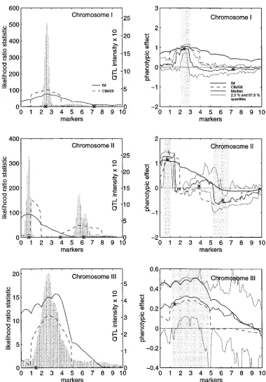
Figure 2.—The

com-plete data analysis. On the left, the results from interval mapping (IM, solid line)

and composite interval

mapping with five back-ground controls (CIM/05, broken line) are shown. Simulated true QTL loca-tions are indicated with an asterix (*). The histogram corresponds to the (approx-imate) posterior QTL inten-sity over the chromosome, with binlength 1 cM. The left (right) y-axis corre-sponds to the likelihood ra-tio statistic (posterior QTL intensity). On the right, cor-responding phenotypic ef-fect estimates are shown. The solid line is the poste-rior median and the grey lines are the 2.5- and 97.5 percent quantiles of the posterior distribution of the phenotypic effect of a puta-tive QTL. Shaded regions are suggested credible in-tervals for QTL localization (see Table 5). The pheno-typic effect estimates (poste-rior median and quantiles) are reliable only in these regions.

the number of QTLs in different chromosomes, for ing the number of QTLs inIby NIqtl, one can calculate

both the complete and the incomplete data, are given various MCMC approximations of that probability as

in Tables 3 and 4. The posterior expectation of the shown in Equation 11 below, where l(s) is the

QTL-number of QTLs in each chromosome (shown in Tables intensity at point s, andlˆ(s) is its estimator:

3 and 4) coincides with the area under the

correspond-ing QTL-intensity curve (in Figures 2 and 3). _P(NI

qtl$ 1| data)≈

1

Ncycs

o

Ncycs

k51

1{l (k)_qPIfor some q}

Perhaps the most natural question to ask in this

con-text is the following: “What is the (posterior) probability ≈ 12 exp{2

#

Ilˆ(s)ds}

that some particular chromosomal area, sayI, contains

≈

_#

Ilˆ(s)ds. (11)

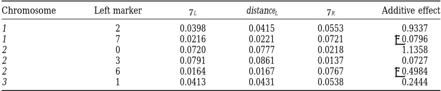
Denot-TABLE 1

The locations and the phenotypic (additive genetic) effects of the simulated QTLs

Chromosome Left marker uL distanceL uR Additive effect

1 2 0.0398 0.0415 0.0553 0.9337

1 7 0.0216 0.0221 0.0721 20.0796

2 0 0.0720 0.0777 0.0218 1.1358

2 3 0.0791 0.0861 0.0137 0.0727

2 6 0.0164 0.0167 0.0767 20.4984

3 1 0.0413 0.0431 0.0538 0.2444

The left column refers to the chromosome in which the considered QTL is. The next column refers to the

nearest left flanking marker of the QTL in the chromosome.uL(uR) is the recombination fraction between

the QTL position and the left (right) flanking marker. distanceLgives the distance (in Morgans) between the

left flanking marker and the QTL position, converted fromuLby using Haldane’s map function.

The last approximation, where the integral on the We do not display empirical threshold values

(corre-sponding to permutation tests) for IM and CIM in Fig-right is actually an expression for the (posterior)

ex-pected number of QTLs inI, is reasonable only if the ures 2 and 3 because they were not the main issues here.

However, the LOD score 3.0 would correspond to the integral is small. Table 5 gives a few such approximations

for some chromosomal areas, based on either the com- likelihood ratio statistic 3.032/log10(e)≈13.82, which

can be used as a rule-of-thumb threshold when examin-plete or the incomexamin-plete data. These regions represent

a moderate to high posterior QTL-intensity region sur- ing the figures (even though it was originally derived

for monogenic traits in human). In practice the CIM

rounding the mode. Making the intervalIlonger will

obviously always increase both the probability P(NIqtl$ method needs a somewhat higher threshold than IM

(Zeng1994). Note that the LRS curves and posterior

1|data) and the expectation E(NIqtl|data), but this will

be at the cost of less accurate localization of the genes. QTL-intensity decrease sharply close to some marker

positions. This is because genotype information con-In other words, given the evidence in the data, there is

always a trade-off between accuracy and probability, just cerning putative QTLs tends to be more accurate close

to markers, and unless a QTL actually coincides with a as in confidence intervals in classical statistical

infer-ence. In this sense, Table 5 represents only one possible marker locus, there will be strong evidence against

plac-ing a QTL in exactly, or very close to, these positions summary of our findings. We have not made an attempt

to establish a standard for forming such intervals or (seeKuittinenet al. 1997).

In Figure 2, the IM and CIM curves, apart from CIM corresponding cut-off points here. Indeed, we think that

the intensity curve in itself is the best summary of the in chromosome 3, contain enough evidence (in the

sense that the LRS is greater than the threshold value information concerning the number of QTLs and their

locations in the chromosome as obtained from the statis- 13.82) of QTL activity. From Figure 2 it can be seen

that our method performs well in all chromosomes, by tical analysis.

TABLE 2

Ranges of the proposal distributions R(.), proposal probabilities, numbers of iterations, and background control markers (BGCs) from other chromosomes,

used in the simulation analyses

R(lq) R(a) R(r2_{) R(bqj) R(ckj) pa}5_{pd Iterations BGCs}

Complete data

Chromosome 1 1.0 cM 0.01 0.01 0.1 0.1 1/3 500,000 2

Chromosome 2 1.0 cM 0.01 0.01 0.1 0.1 1/3 500,000 0,1,6

Chromosome 3 2.0 cM 0.01 0.01 0.1 0.1 1/3 1,000,000 2

Incomplete data

Chromosome 1 1.0 cM 0.01 0.01 0.1 0.1 1/3 500,000 2,3

Chromosome 2 1.0 cM 0.01 0.01 0.1 0.1 1/3 500,000 1,6

Chromosome 3 2.0 cM 0.01 0.01 0.1 0.1 1/3 1,500,000 3

Notation is as follows: R(lq) is the range of proposals for the QTL location parameters, R(a) for the regression

mean, R(r2_{) for the residual variance, R(b}

qj) for the regression coefficients of the QTL genotypes, and R(ckj)

Figure 3.—The

incom-plete (30% of genotypes missing) data analysis. On the left, the results from in-terval mapping (IM, solid line) and composite inter-val mapping with five back-ground controls (CIM/05, broken line) are shown. Simulated true QTL loca-tions are indicated with an asterix (*). The histogram corresponds to the (approx-imate) posterior QTL inten-sity over the chromosome, with binlength 1 cM. The left (right) y-axis corre-sponds to the likelihood ra-tio statistic (posterior QTL intensity). On the right, cor-responding phenotypic ef-fect estimates are shown: the solid line is the posterior median and the grey lines are the 2.5- and 97.5-per-cent quantiles of the poste-rior distribution of the phe-notypic effect of a putative QTL. Shaded regions are suggested credible intervals for QTL localization (see Table 5). The phenotypic effect estimates (posterior median and quantiles) are reliable only in these re-gions.

giving well localized high intensities for QTLs close to estimated separately with a permutation test (Churchill

andDoerge 1994) or by bootstrapping]. Our method

their true locations. Note that the highest

QTL-intensi-ties are often found near the modes of CIM or IM curves. gave posterior credible intervals for the phenotypic

ef-fects in all cases. The weakest QTLs in chromosomes 1 and 2 remained

undetected by any of these methods, apparently because In the case of incomplete data, the mode of the

inten-sity given by our method differs by 12 cM from the of their small phenotypic effects. All three methods

estimated the phenotypic effect of the most influential simulated true location in chromosome 3 (Figure 3).

This is apparently a consequence of reduced genotype QTLs very accurately, but IM and CIM/05 do not give

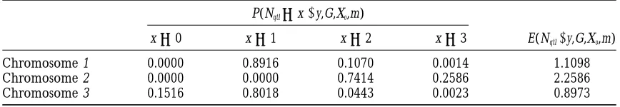
TABLE 3

The posterior distribution of the number of QTLs and its posterior expectation in the three chromosomes (complete genotype data)

P(Nqtl5x|y,G,Xo,m)

x50 x51 x52 x53 E(Nqtl|y,G,Xo,m)

Chromosome 1 0.0000 0.8916 0.1070 0.0014 1.1098

Chromosome 2 0.0000 0.0000 0.7414 0.2586 2.2586

Chromosome 3 0.1516 0.8018 0.0443 0.0023 0.8973

weak phenotypic effect attributable to this particular At the “left end” of chromosome 2, we obtained the

one-lod-support interval [2.9 cM, 9.0 cM] when using QTL. Note in this case the low maximal level of the

posterior QTL-intensity, compared to the levels reached the IM, and [10.0 cM, 11.9 cM] when using the CIM

method. The latter interval is actually so narrow that in the other two chromosomes.

For a more explicit comparison of the three methods, the true QTL at 7.77 cM falls just outside it. The

poste-rior QTL-intensity in this region is concentrated almost

one-lod-support intervals (see Ott 1991, pp. 66–67)

were determined around the modes of the IM and CIM/ completely on the interval I 5 [4 cM, 10 cM] which

again contains the true QTL. At the “right end” of chro-05 curves estimated from the complete data. The

thresh-old values defining the one-lod-support intervals are the mosome 2, the LRS curve arising from CIM is bimodal,

resulting in two overlapping one-lod-support intervals, maximal value (the mode) minus 1.0 LOD (i.e.,

2/log10(e) units in the LRS scale). An alternative would [53.6 cM, 59.6 cM] and [52.9 cM, 67.3 cM]. The shorter

CIM interval is so narrow that it does not contain the have been to estimate confidence intervals for the QTL

locations, by applying a permutation test (seeChurch- true QTL at 61.67 cM, but the wider one does. In this

case, a natural choice for a Bayesian credible region

ill and Doerge 1994) or by bootstrapping, as in

Visscheret al. 1996b. The results from the comparison would be the interval I5 [53 cM, 68 cM], which is

very close to that obtained by CIM and for which the are summarized in Table 6. (The numerical accuracy

of the estimated support interval depends on the chosen posterior probability of there being at least one QTL

in the region is 0.64. The IM method failed to reveal step size which specifies how frequently the LRS is

evalu-ated along the chromosome.) any statistically significant QTL activity in this part of

chromosome 2. Considering first the complete data set and the first

chromosome with the LRS evaluated at every 0.1 cM, In chromosome 3, we obtained the one-lod-support

interval [0.0 cM, 39.8 cM] with the IM method. With the we obtained the one-lod-support interval [23.0 cM, 29.2

cM] using the IM, and [21.6 cM, 27.3 cM] using the CIM CIM method, we could not determine a corresponding

support interval because the maximum LRS value was method. The latter almost coincides with the interval

I5[21 cM, 28 cM] (see Tables 5 and 6), obtained from less than the critical value LOD 3.0. Because of the small

phenotypic effect of the simulated QTL, the Bayesian Figure 2 so that it contains practically all moderate to

high posterior QTL-intensity values. All these intervals method did not localize this QTL as well as in

chromo-somes 1 and 2. Perhaps a natural interval to suggest, if covered the true QTL at 24.15 cM. The posterior

proba-bility that the regionIcontains at least one QTL is 0.63. at all, would be [0 cM, 37 cM], which would be nearly

identical to the interval suggested by the IM-analysis The true phenotypic effect of the second QTL (at 72.21

cM) in chromosome 1 was so small that this QTL was and which would cover 90.2 percent of the total area

under the QTL-intensity curve in that chromosome. not detected by any of the three methods discussed

here. Whenever possible, all three methods estimated the

TABLE 4

The posterior distribution of the number of QTLs and its posterior expectation in the three chromosomes (incomplete genotype data)

P(Nqtl5x|y,G,Xo,m)

x50 x51 x52 x53 E(Nqtl|y,G,Xo,m)

Chromosome 1 0.0000 0.7803 0.2058 0.0139 1.2336

Chromosome 2 0.0000 0.0000 0.7966 0.2034 2.2034

TABLE 5

Approximate (posterior) probability (12exp{2

#

I Length (I) P(NIqtl$1|data) E(NIqtl|data)

Complete data

Chromosome 1 [21 cM, 28 cM] 7 cM 0.63 0.9901

Chromosome 2 [ 4 cM, 10 cM] 6 cM 0.63 0.9940

Chromosome 2 [53 cM, 68 cM] 15 cM 0.64 1.0148

Chromosome 3 [ 0 cM, 37 cM] 37 cM 0.55 0.8093

Incomplete data

Chromosome 1 [21 cM, 30 cM] 9 cM 0.64 1.0106

Chromosome 2 [ 3 cM, 11 cM] 8 cM 0.63 0.9960

Chromosome 2 [52 cM, 68 cM] 16 cM 0.63 1.0019

Chromosome 3 [12 cM, 48 cM] 36 cM 0.57 0.8434

The (posterior) expected number of QTLs inI, calculated as the integral of the QTL intensity overIis

also determined.

locations of the QTLs fairly well (see Table 6). In all For the estimation of the parameters (seeappendix a)

we use the Metropolis-Hastings algorithm with “revers-these analyses the Bayesian estimates (posterior

medi-ans) of individual phenotypic effects were close to the ible jumps” (Green1995) between models with

differ-ent numbers of QTLs. In the case of more than one true values, and they were practically the same as what

was obtained when applying the CIM method. In this QTL, this construction improved the mixing properties

of the sampler when compared to a single-QTL model respect, the IM method turned out to be much inferior.

The results from analysing the incomplete data were (results not shown). The effects on the QTLs in other

chromosomes are taken into account indirectly, largely similar, see Tables 5 and 6, and Figure 3 for

details. The main difference was that the one-lod-sup- through nearby markers. When the genotype of a

marker is missing, information from surrounding mark-port intervals become somewhat wider, as did the

corre-sponding Bayesian credible regions. The differences ers is utilized by applying the conditional probabilities

as specified in Equation 5. were not very large, however.

The main advantage in using Bayesian, instead of the more traditional frequentist inferential methods, is that DISCUSSION

they enable the analyst to quantify probabilistically the uncertainty involved in each claim made about QTLs, We have presented here a novel method for high

resolution mapping of multiple QTLs and for the esti- without needing to use problematic mental constructs

such as “the relative frequency of incorrect decisions mation of their phenotypic effects, using the general

framework of Bayesian variable dimensional models. made in a long sequence of trials repeated under similar

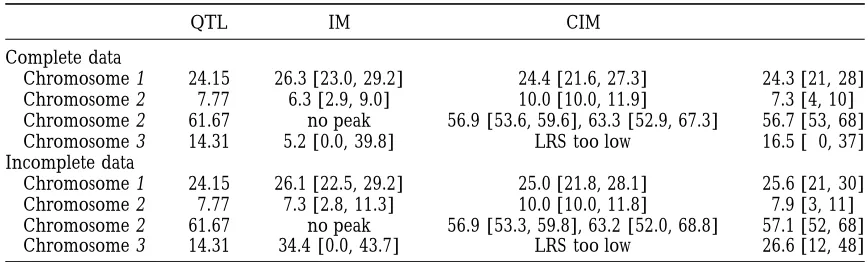
TABLE 6

True locations (QTL), estimated locations and one-lod-support intervals for IM and CIM, and Bayesian point estimates (modes of the QTL intensity) together with the support

intervals (I) from Table 5

QTL IM CIM I

Complete data

Chromosome 1 24.15 26.3 [23.0, 29.2] 24.4 [21.6, 27.3] 24.3 [21, 28]

Chromosome 2 7.77 6.3 [2.9, 9.0] 10.0 [10.0, 11.9] 7.3 [4, 10]

Chromosome 2 61.67 no peak 56.9 [53.6, 59.6], 63.3 [52.9, 67.3] 56.7 [53, 68]

Chromosome 3 14.31 5.2 [0.0, 39.8] LRS too low 16.5 [ 0, 37]

Incomplete data

Chromosome 1 24.15 26.1 [22.5, 29.2] 25.0 [21.8, 28.1] 25.6 [21, 30]

Chromosome 2 7.77 7.3 [2.8, 11.3] 10.0 [10.0, 11.8] 7.9 [3, 11]

Chromosome 2 61.67 no peak 56.9 [53.3, 59.8], 63.2 [52.0, 68.8] 57.1 [52, 68]

Chromosome 3 14.31 34.4 [0.0, 43.7] LRS too low 26.6 [12, 48]

Figure 4.—The sample

path k→N(k)

qtl from a

simula-tion trial of 1,000,000 itera-tions with complete data set (Chromosome 3).

conditions.” The transformation of the prior distribu- rior QTL-intensity captures the essential information

about their number and positions in an easily interpret-tion into the posterior through Bayes’ formula,

corre-sponds directly to the natural intuition of “learning from able probabilistic form. In this way we can avoid

com-pletely the difficult inferential problems concerning the the data.” Depending on the goals of the study, the

specification of the prior can be “neutral” if the goal is “correct” threshold values of a LOD score (or a LRS)

which arise in testing multiple QTL hypotheses. More-to present a statistical summary of the information in

the data, or, if available, it can also reflect an expert’s over, our method does not appear to produce false

positives easily, as one can expect to get a low QTL-prior knowledge about unobserved quantities, in which

case the posterior will be a synthesis of such expert intensity in regions where there is no, or is only little,

QTL activity. knowledge and empirical evidence coming from the

data. Another major advantage of the Bayesian ap- The performance of our method was compared to

interval mapping (IM) and composite interval mapping proach is the relative ease by which missing data (such as

missing genotypes) problems can be handled, together (CIM) by using a simulated backcross population of 250

offspring. A second data set was obtained by randomly with the estimation of all other unobservables. Finally,

the application of MCMC methods gives considerable deleting 30 percent of the marker genotypes in the

complete set. freedom in building large hierarchical statistical models

corresponding to the analyst’s perception of the under- In the execution of the MCMC sampling we used an

overparametrized regression model which has one extra lying genetic structures and dependencies.

The results of the statistical analysis are summarized coefficient for each QTL and for each background

con-trol locus. Therefore the model intercept and the geno-by two new measures: the posterior QTL-intensity,

con-sidered as a function of its location in the chromosome, typic coefficients are not identifiable as such, but their

contrasts (phenotypic effects) are. We also tested the and the posterior distribution of the phenotypic effect

of the corresponding putative QTL. Such probabilistic alternative updating scheme used by Satagopanand

Yandell(1996) where, when the number of QTLs was

summary measures seem to correspond directly to the

immediate objectives of QTL mapping, that is, localizing proposed to be changed, its effect was first balanced

against a corresponding change in the overall mean. the important QTLs in different chromosomes and

esti-mating their effects on the phenotype(s). In particular, Our overparametrized model seemed to have better

mixing properties, however. in situations where one can expect that there are several

compu-tational effort and will, in practice, need the capacity mented version is currently being developed. The pres-ent framework will be extended later to cover outbred of a workstation. To ensure sufficient mixing, we

per-formed some relatively long test runs before a final QTL linecross and (human) pedigree data. Epistatic effects

(interactions between QTLs) and multiple trait analysis analysis. Another possibility is to apply some diagnostic

tools, such as CODA (Bestet al. 1995). Because we ran would also be worth considering in the future.

long simulation trials, no sampled values were rejected _{M.S. thanks}Kari Auranen, Jukka RantaandDario Gasbarra

because of burn-in. The mixing properties of the sam- for many useful discussions about Metropolis-Hastings algorithms, and

Matti Taskinenfor helpful hints in the programming and computer

pling algorithm do not seem to be very sensitive to

work. We are also grateful toOuti Savolainen, Leena Peltonen,

the prespecified proposal probabilities. In the case of

Claus Vogl, Janne Pitk¨ aniemi, Pekka Uimariand four anonymous

adding or deleting a QTLs, the only restriction appeared

referees for their constructive comments on an earlier version of the

to be that the proposal probabilities of changing the _{paper. This work was supported by a research grant from the Academy}

dimension should not be too small. As an illustration of Finland.

of the degree of mixing which was typically

encoun-tered, we show (Figure 4) how Nqtl was varying in a

simulation run of length 1,000,000. In the final runs,

LITERATURE CITED the observed rejection rates for both adding and

delet-ing steps varied between 0.998 and 0.999. By compari- Arjas, E.,_andD. Gasbarra_{, 1994 Nonparametric Bayesian}

infer-ence from right censored survival data using the Gibbs sampler. son, the rejection rates for updating QTL locations were

Statist. Sinica 4: 505–524.

rather low in general because the proposals were usually _{Basten, C. J., B. S. WeirandZ.-B. Zeng, 1996 QTL Cartografer,}

limited to a fairly narrow interval around the current the reference manual and tutorial for QTL mapping. (available

at http://statgen.ncsu.edu.) value. (Larger jumps were allowed when a QTL was

Besag, J., P. Green, D. HigdonandK. Mengersen, 1995 Bayesian

either deleted or added.) _{computation and stochastic systems. Statist. Sci. 10: 3–66.}

An important issue which has so far come up only Best, N. G., M. K. CowlesandS. K. Vines, 1995 CODA:

Conver-gence Diagnosis and Output Analysis software for Gibbs Sampler implicitly in our analysis is that the number of QTLs

output: Version 0.3. Cambridge: Medical Research Council

Bio-and their phenotypic effects cannot be considered in _{statistic Unit.}

isolation from each other. The idea that any gene with Casella, G.,andE. I. George, 1992 Explaining the Gibbs sampler.

American Statistician 46: 167–174. a non-zero effect on phenotypes is a QTL which in

Chib, S.,andE. Greenberg, 1995 Understanding the

Metropolis-principle could be detected from data seems like an

Hastings algorithm. American Statistician 49: 327–335.

idealization far from reality, and as a consequence, “the Churchill, G. A.,andR. W.Doerge, 1994 Empirical threshold

values for quantitative trait mapping. Genetics 138: 963–971. correct number of QTLs” will exist as an objectively

Dempster, A. P., N. M. LairdandD. B. Rubin, 1977 Maximum

defined quantity only in simulated data. Here we have

likelihood from incomplete data via the EM algorithm. J. Roy.

controlled this problem by bounding the number of _{Statist. Soc., Ser. B. 39: 1–38.}

Geman, S.,andD. Geman, 1984 Stochastic relaxation, gibbs

distribu-QTLs in each chromosome by a given constant. An

tion, and the Bayesian restoration of images. IEEE Trans. Pattn. alternative would be to modify our method by paying

Anal. Mach. Intell. 6: 721–741.

attention only to influential QTLs, in the sense that Geyer, C. J.,_{1992 Practical Markov Chain Monte Carlo. Statist. Sci.}

their phenotypic effect exceeds some given threshold 7:473–511.

Geyer, C. J.,_{1996 Likelihood inference for spatial point processes.}

T. The only change this would make into our formulas

(available at http://www.stats.bris.ac.uk/MCMC/)

is that, in Equations 9 and 10, we would have to add Green, P. J.,_{1995 Reversible jump Markov Chain Monte Carlo}

com-into indicators the restriction|b(k)

q 22 b(k)q1|$T. putation and Bayesian model determination. Biometrika 82: 711–

732. Another question we have not discussed is how to

Guo, S. W.,andE. A. Thompson, 1992 Monte Carlo method for

choose the markers which are to be used as covariates _{combined segregation and linkage analysis. Am. J. Hum. Genet.}

in the analysis. Instead of using the results from a prelim- 51:1111–1126.

Hackett, C. A.,_andJ. I. Weller,_{1995 Genetic mapping of}

quantita-inary stepwise regression analysis as we have done here,

tive trait loci for traits with ordinal distributions. Biometrics 51:

one could “learn” from Bayesian QTL analyses of other _1252–1263.

chromosomes and choose certain markers from high Haley, C. S.,_andS. A. Knott_{, 1992 A simple regression method}

for mapping quantitative trait loci in line crosses using flanking posterior QTL-intensity areas as QTL representatives

markers. Heredity 69: 315–324.

(background controls). Alternatively, one could choose _{Haley, C. S., S. A. Knott,andJ.-M. Elsen, 1994 Mapping}

quantita-covariates from amongst a set of candidate genes in case tive trait loci in crosses between outbred lines using least squares.

Genetics 136: 1195–1207. such genes are available. A final possibility would be to

Hastings, W. K._{, 1979 Monte Carlo sampling methods using Markov}

consider the entire genome in a single variable dimen- _{chains and their applications. Biometrika 57: 97–109.}

sional QTL analysis, always using the “current” QTLs as Jansen, R. C.,_{1993 Interval mapping of multiple quantitative trait}

loci. Genetics 135: 205–211,

controls (SatagopanandYandell1996;Stephensand

Jansen, R. C._{, 1996 A General Monte Carlo method for mapping}

Fisch 1996). For this our method would need some

multiple quantitative trait loci. Genetics 142: 305–311.

adjustments, however. Jansen, R. C.,_andP. Stam_{, 1994 High resolution of quantitative}

traits into multiple loci via interval mapping. Genetics 136: 1447– An initial version of the program source code (written

1455. in C language) is freely available for research purposes

Kruglyak, L.,_andE. S. Lander_{, 1995 A Nonparametric approach}

from Rolf Nevanlinna Institute’s web page (http:// _{for mapping quantitative trait loci. Genetics 139: 1421–1428.}

Kuittinen, H., M. J. Sillanpa¨ a¨, andO. Savolainen_{, 1997 Genetic}

docu-basis of adaptation: flowering time in Arabidopsis Thaliana. Zeng, Z.-B., 1994 Precision mapping of quantitative trait loci.

Genet-Theor. Appl. Genet. 95: 573–583. ics 136: 1457–1468.

Lander, E. S.,andD. Botstein, 1989 Mapping Mendelian factors

Communicating editor:Z-B. Zeng

underlying quantitative traits using RFLP linkage maps. Genetics

121:185–199.

Lincoln, S., M. Daly,_andE. S. Lander_{, 1992 Mapping genes}

con-trolling quantitative traits with MAPMAKER/QTL 1.1 Whitehead

APPENDIX A: ESTIMATION OF MODEL PARAMETERS Institute Technical Report. 2nd edition.

Metropolis,N., A. W. Rosenbluth, M. N. Rosenbluth, A. H. VIA MARKOV CHAIN MONTE CARLO

Teller,_andE. Teller_{, 1953 Equation of state calculations by}

fast computing machines. J. Chem. Phys. 21: 1087–1092. Markov chain Monte Carlo (MCMC) methods enable

Ott, J.,_{1991 Analysis of Human Genetic Linkage. Revised edition. The}

one to calculate expectations with respect to the poste-John Hopkins University Press, Baltimore.

rior in an approximate manner in situations where

com-Richardson,S., _and P. J. Green_{, 1997 On Bayesian analysis of}

mixtures with an unknown number of components. J. Roy. Statist. _{putation by traditional methods, because of the high}

Soc., Ser. B, 59: 731–792. _{dimension of the parameter space, would be}

compli-Satagopan, J. M.,andB. S. Yandell, 1996 Estimating the number of

cated or impossible. In MCMC, each expectation is ap-quantitative trait loci via Bayesian model determination. Special

Contributed Paper Session on Genetic Analysis of Quantitative _{proximated by a sample average where the sample is}

Traits and Complex Diseases, Biometric Section, Joint Statistical _{drawn by simulation from an ergodic Markov chain}

con-Meetings, Chicago, IL. (available at ftp://ftp.stat.wisc.edu/pub/

structed in such a way that its limiting distribution coin-yandell/revjump.html)

Satagopan, J. M., B. S. Yandell, M. A. Newton,andT. C. Osborn, cides with the posterior. The fact that the number of

1996 A Bayesian approach to detect quantitative trait loci using _{QTLs has not been fixed in advance, and is actually}

Markov Chain Monte Carlo. Genetics 144: 805–816.

estimated in conjunction with the other model

parame-Smith, A. F. M.,1996 Bayesian curves and CARTs. First European

Conference on Highly Structured Stochastic Systems, Rebild, May _{ters, leads us to consider this problem within the general}

1996.

framework of variable dimensional parameter

estima-Smith, A. F. M.,_andG. O. Roberts_{, 1993 Bayesian computation}

tion. via the Gibbs sampler and related Markov Chain Monte Carlo

methods. J. Roy. Statist. Soc., Ser. B, 55: 3–23. _{We have preferred to use the Metropolis-Hastings}

Stephens, D. A.,andR. D. Fisch, 1996 Bayesian analysis of

quantita-algorithm (M-H) instead of its special case, the Gibbs tive trait locus data using reversible jump Markov chain Monte

sampler. The main motivation behind this choice has Carlo. Technical report. (available at http://www.ma.ic.ac.uk/

statistics/techrep.html) _{been that the M-H algorithm is so easy to implement,}

Stephens, D. A.,andA. F. M. Smith, 1993 Bayesian inference in

without needing to work with analytically involved full multipoint gene mapping. Ann. Human Genet. 57: 65–82.

Tai, J. J.,1989 Application of Bayesian decision procedure to the conditional distributions. An additional bonus of M-H

inference of genetic linkage. J. Am. Statist. Assoc. 84: 669–673. _{is its greater flexibility and the relative ease by which it}

Tanksley, S. D.,1993 Mapping polygenes. Annu. Rev. Genet. 27:

can be extended to more complex designs and pedigree 205–233.

Thomas, D. C.,andV. Cortessis,1992 A Gibbs sampling approach structures.

in linkage analysis. Hum. Hered. 42: 63–76.

For algorithmic reasons (mixing properties), we do

Thomas, D. C.,andW. J. Gauderman,1995 Gibbs sampling

meth-not use any constraints for gemeth-notypic coefficients, even ods in genetics, pp. 419–440 in Markov Chain Monte Carlo in

Practice, edited byW. R. Gilks, S. RichardsonandD. J. Spiegel- _{if this kind of overparametrization represents an} uncom-halter._{Chapman & Hall, London.}

mon modeling practice. Genotypic coefficients are here

Thompson, E. A.,1994 Monte Carlo likelihood in genetic mapping.

not identifiable as such, but their contrasts can be esti-Statist. Sci. 9: 355–366.

Uimari, P.,andI. Hoeschele,1997 Mapping linked quantitative _mated.

trait loci using Bayesian analysis and Markov chain Monte Carlo

FollowingGreen’s(1995) construction of a Markov

algorithms. Genetics 146: 735–743.

chain with reversible jumps, we apply acceptance

proba-Uimari, P., G. Thaller_{, and}I. Hoeschele,_{1996a The use of}

multi-ple markers in a Bayesian method for mapping quantitative trait _{bilities of the form min{ 1 , (posterior ratio)3(proposal}

loci. Genetics 143: 1831–1842.

ratio) 3 (Jacobian)}. Throughout our consideration

Uimari, P., Q. Zhang, F. Grignola, I. Hoeschele, andG. Thaller,

1996b Analysis of QTL workshop I Granddaughter design data here, the Jacobian is one, being the determinant of an

using least-squares, residual maximum likelihood and Bayesian _{identity matrix. This is because the location(s) of}

ex-methods. J. QTL 1996: 2, art. 7.

isting QTL(s) do not determine the location of a

pro-Utz, H. F.,_andA. E. Melchinger_{1996 PLABQTL: A program for}

composite interval mapping of QTL. J. Quant. Trait Loci 2: 7. _{posed new QTL, nor does the deletion of one QTL}

van OoijenJ. W., _andC. Maliepaard, _{1996 Plant Genome IV.}

influence the position(s) of the remaining QTL(s). In Abstract at: http://probe.nalusda.gov:8000/otherdocs/pg/pg4/

the following, we describe the steps of our Metropolis-abstracts/p316.html.

Visscher, P. M., C. S. Haley, andS. A. Knott, 1996a Mapping Hastings-Green cycle. Initial values of the number of

QTLs for binary traits in backcross and F2 populations. Genet. _{QTLs, of their locations, as well as the Poisson meanl,}

Res., Camb. 68: 55–63.

the maximal number of QTLs allowed and the ranges

Visscher, P. M., R. Thompson_{, and}C. S. Haley_{, 1996b Confidence}

intervals in QTL mapping by bootstrapping. Genetics 143: 1013– _{of the uniform priors, are all given by the analyst (see}

1020.

simulation analysis). Initial values of the regression

pa-Xu, S.,andW. R. Atchley, 1996 Mapping quantitative trait loci for

rameters are generated to be close to the center of their complex binary diseases using line crosses. Genetic 143: 1417–

1424. _{prior range. Initial values for the QTL genotypes and}

Zeng, Z.-B._{, 1993 Theoretical basis for separation of multiple linked}

missing marker genotypes are generated from their pri-gene effects in mapping quantitative trait loci. Proc. Natl. Acad.