ABSTRACT
SMART, LINDSEY SUZANNE. Rising Seas and the Changing Coastal Landscape: Modeling Land Change Pattern and Social Process to Quantify the Socio-Ecological Impacts of Sea Level Rise. (Under the direction of Dr. Ross K. Meentemeyer and Dr. Jordan W. Smith).
Rising Seas and the Changing Coastal Landscape: Modeling Land Change Pattern and Social Process to Quantify the Socio-ecological Impacts of Sea Level Rise
by
Lindsey Suzanne Smart
A dissertation submitted to the Graduate Faculty of North Carolina State University
in partial fulfillment of the requirements for the degree of
Doctor of Philosophy
Forestry and Environmental Resources
Raleigh, North Carolina 2019
APPROVED BY:
_______________________________ _______________________________ Dr. Ross K. Meentemeyer Dr. Jordan W. Smith Co-Chair of Advisory Committee Co-Chair of Advisory Committee
_______________________________ _______________________________ Dr. Erin Seekamp Dr. Helena Mitasova
ii DEDICATION
iii BIOGRAPHY
iv ACKNOWLEDGMENTS
v TABLE OF CONTENTS
LIST OF TABLES ... viii
LIST OF FIGURES ... ix
CHAPTER 1: Introduction ... 1
1.1. INTRODUCTION ... 1
1.2. REFERENCES ... 6
CHAPTER 2: Coastal Biomass Loss from Sea Level Rise Quantified with Repeat Lidar Surveys ... 8
2.1. INTRODUCTION ... 8
2.2. METHODS ... 11
2.2.1. Study system ... 11
2.2.2. Field data collection ... 12
2.2.3. Lidar data processing ... 14
2.2.4. Lidar vegetation metrics ... 15
2.2.5. Landsat data processing ... 18
2.2.6. Predictive modeling ... 19
2.2.7. Evaluation of model performance ... 20
2.3. RESULTS ... 20
2.3.1. Plot level estimates of biomass change ... 20
2.3.2. Predictive model performance ... 21
2.3.3. Contribution of vegetation metrics ... 27
2.3.4. Coastal forest declines and aboveground biomass change ... 30
2.4. DISCUSSION ... 34
2.4.1. Heterogeneity in the magnitude and spatial patterns of aboveground biomass change ... 34
2.4.2. Multi-sensor data integration proves beneficial ... 36
2.4.3. Challenges of repeat measures ... 38
2.5. CONCLUSION ... 40
2.6. REFERENCES ... 41
CHAPTER 3: Modeling the Relative Contributions of Sea Level Rise and Land-use Change to Forest Carbon Decline ... 49
3.1. INTRODUCTION ... 49
3.1.1. Impacts of sea level rise on carbon storage in freshwater-dependent coastal ecosystems ... 50
3.1.2. Anthropogenic- and disturbance-impacts on carbon ... 52
3.1.3. Quantifying drivers of carbon flux in dynamic systems ... 53
3.2. METHODS ... 54
3.2.1. Study system ... 54
vi
3.2.3. Driver variables and data preparation ... 59
3.2.4. Statistical modeling approach ... 62
3.2.5. Evaluation of model performance ... 63
3.2.6. Predicting future aboveground carbon declines ... 64
3.3. RESULTS ... 65
3.3.1. Statistical modeling of coastal terrestrial aboveground carbon declines ... 65
3.3.2. Future coastal terrestrial carbon declines ... 72
3.4. DISCUSSION ... 74
3.4.1. Ecological implications ... 75
3.4.2. Future scenarios ... 76
3.4.3. Model limitations ... 77
3.5. CONCLUSION ... 78
3.6. REFERENCES ... 80
CHAPTER 4: Socio-spatial Factors Determine Landowners’ Interest in Sea Level Rise Adaptation Programs ... 86
4.1. INTRODUCTION ... 86
4.1.1. Coastal sea level rise adaptation in the Southeast U.S. ... 87
4.1.2. Factors influencing landowners’ adaptive decision-making behaviors ... 89
4.1.3. Influence of social norms, social networks, and information diffusion on adaptive behaviors ... 90
4.1.4. Choice under risk – landowner climate change risk perceptions ... 94
4.1.5. Spatial context as a driver of program adoption ... 95
4.2. METHODS ... 96
4.2.1. Study system ... 96
4.2.2. Survey sample frame... 97
4.2.3. Data collection ... 98
4.2.4. Survey instrument and measures ... 99
4.2.4.1. Discrete choice experiment design ... 99
4.2.4.2. Scenario attributes ... 100
4.2.4.3. Individual attributes ... 102
4.2.5. Analysis of discrete choice experiment ... 102
4.3. RESULTS ... 103
4.3.1. Socio-demographic characteristics ... 103
4.3.2. Perception of risk among survey respondents ... 105
4.3.3. Results from the discrete choice experiments ... 106
4.4. DISCUSSION ... 114
4.4.1. Individual and property characteristics influencing participation ... 114
4.4.2. Program attributes associated with adaptation program interest ... 115
4.4.3. Risk perception ... 116
4.4.4. Social norms and information networks ... 117
4.4.5. Landscape position and spatial context... 119
4.4.6. Landscape-scale implications for adaptation ... 120
4.5. CONCLUSION ... 120
vii
APPENDICES ... 133
Appendix A ... 134
Appendix B ... 143
viii LIST OF TABLES
Table 2.1 Allometric biomass equations for woody and herbaceous vegetation ... 13 Table 2.2 Acquisition parameters for lidar surveys in 2001 and 2014. Lidar data collected
as part of the North Carolina Floodplain Mapping Program ... 15 Table 2.3 Predictor variables derived from lidar data by binning the appropriate statistics
at selected grid resolution (e.g. 12-m or 30-m resolution as in this analysis). ... 16 Table 2.4 Summary statistics of field and lidar data for plots across the three vegetation
communities in 2001 and 2014. All values are in meters. ... 17 Table 2.5 Specifications of Landsat imagery for 2001 and 2014 along with Palmer
Drought Severity Index (PDSI) for relative dryness that ranges from -10 (dry) to 10 (wet). ... 18 Table 2.6 Metrics derived from spectral bands of Landsat data ... 18 Table 2.7 Model performance measures and statistics for each of the tested models:
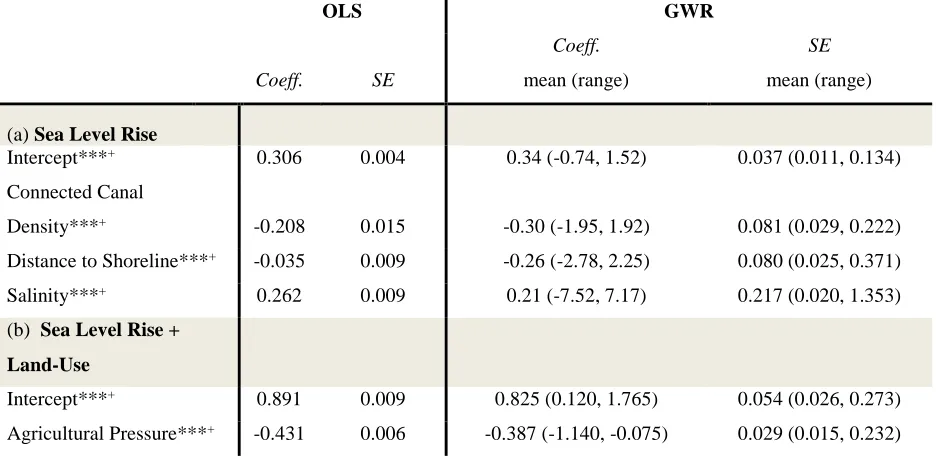
12-m resolution 12-model with lidar data only, 30-12-m resolution data with lidar only, and 30-m resolution integrated model with both lidar and Landsat data. ... 29 Table 3.1 Predictor variables used in both global and local regression models ... 59 Table 3.2 Global and local regression model results for Sea Level Rise + Land-use
Model and Sea Level Rise Model ... 65 Table 4.1 Summary of socio-demographic and property characteristics of survey
respondents ... 104 Table 4.2 Estimates from the mixed effects logistic regression predicting landowners’
ix LIST OF FIGURES
Figure 1.1 Conceptual diagram of research questions situated within the socio-ecological systems framework as adapted from Ostrom, 2009. Dissertation research question 1(RQ1), situated fully within the ecological systems component of the framework, quantifies landscape-scale coastal aboveground biomass change over a 13-year period. Dissertation research question 2 (RQ2) examines the potential drivers of aboveground biomass change – natural disturbance drivers, sea level rise drivers, and land-use or anthropogenic drivers. By examining human influences on the landscape, I’ve situated this research question outside of the ecological systems component as it begins to explore the interactions between humans and landscape condition. Dissertation research question 3 (RQ3) examines the socio-spatial factors driving landowners’ willingness to enroll in adaptation programs. We examine the influence of the landscape on individuals’ perceived risk and adaptive behaviors. As such, we’ve situated this research question slightly outside of the social systems component of the framework as it quantifies the influence of landscape context on the behavioral intentions of landowners as they respond to the impacts from sea level rise ... 5 Figure 2.1 The Albemarle-Pamlico Peninsula is located in eastern North Carolina of the
United States. Ninety-eight random field plots were established across five sites (with 21 plots in each site except for Palmetto Peartree, which lacked marsh communities) among three vegetation communities: forest, transition forest, and marsh. ... 13 Figure 2.2 An example 450m2 forested field plot in the Palmetto Peartree study area,
showing the difference in density between (a) 2001 and (b) 2014 lidar data. Dark grey color signifies points classified as vegetation and black color signifies points classified as ground. ... 14 Figure 2.3 Comparison of field data and lidar data kernel density distributions for
maximum vegetation height and mean vegetation height at the 98 study site plots ... 17 Figure 2.4 Mean field-measured aboveground biomass by community type and year. The
* denotes a statistically significant difference between years (p<0.05). ... 21 Figure 2.5 Observed biomass plotted against the Random Forest imputed biomass
estimates, derived from 1,000 regression trees for (a) 2001 and (b) 2014. ... 23 Figure 2.6 Observed biomass plotted against the Random Forest imputed biomass
x Figure 2.7 Total aboveground biomass maps derived from the 30-m resolution integrated
model (a) 2001 and (b) 2014. Standard deviation for (c) 2001 and (d) 2014 aboveground biomass Random Forest imputation, derived from 1,000 permutations of the 30-m resolution integrated model. Coefficient of variation for (e) 2001 and (f) 2014 aboveground biomass Random Forest imputation, derived from 1,000 permutations of the 30-m resolution integrated model ... 26 Figure 2.8 Permutation importance of predictor variables derived from 1,000
permutations of the final fitted Random Forest models for (a) 2001 and (b) 2014. Percent increase in MSE is the increase in mean square error of predictions as a result of each variable being randomly permuted. The higher the increase, the more important the variable. Black color indicates contribution is statistically significant ... 28 Figure 2.9 Map of biomass change from the 30-m resolution integrated models for the
study area, derived by subtracting the 2001 imputed Random Forest biomass map from the 2014 imputed Random Forest biomass map. Inset maps of biomass change for (a) eastern portion of the study area, near Stumpy Point, (b) northern portion of the study area at the mouth of the Alligator River, and (c) southeastern portion of the study area in Gull Rock Game Land ... 31 Figure 2.10 Vegetation class mapping using the RF model for (a) 2001 and (b) 2014 and
(c) change analysis between years ... 32 Figure 2.11 Relationship between aboveground biomass change and vegetation
classification change between 2001 and 2014. Mean AGB change was sampled using a systematic grid of points with a minimum distance between points of 500 m. Croplands, fires, and developed areas were excluded from the estimates. On the secondary axis is mean distance to the estuarine shoreline (km) for each class. Area (km2) and percent of natural landscape for each
transition type are included under each class transition ... 33 Figure 2.12 Relationship between field biomass change between 2001 and 2014 at the plots
and predicted biomass change from (a) the 12-m resolution models; (b) the 30-m resolution lidar only 30-models; (c) the 30-30-m resolution Landsat only 30-models; and (d) 30-m resolution integrated models ... 34 Figure 3.1 Map of study area. Land cover obtained from the 2011 National Land Cover
Dataset (NLCD). Inset map shows the portion of the peninsula that is less than 1 m in elevation as measured from a digital elevation model ... 56 Figure 3.2 (a) Map of Landsat-lidar derived aboveground biomass change. (b) Fractional
carbon decline as derived from map of aboveground biomass change ... 58 Figure 3.3 Schematic of response variable calculation. Fractional carbon decline is the
xi (colored cells/total number of cells; 0.67) within each modeling unit
experiencing decline ... 59 Figure 3.4 Relative importance for fractional decline with 95% bootstrap confidence
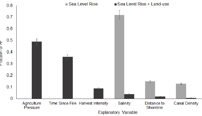
intervals using method Lindemann, Merenda, and Gold (1980). Metrics are normalized to sum to 100%. Results are presented for the FULL model (R2 = 36.94%) and the SLR (sea level rise) Model (R2= 5.36%) ... 67
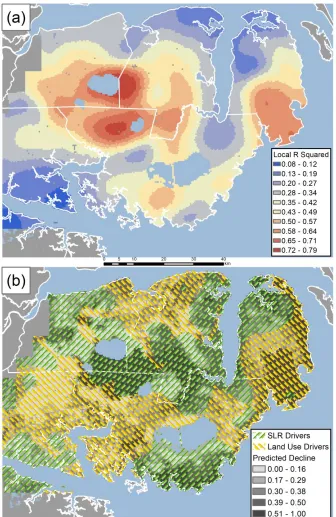
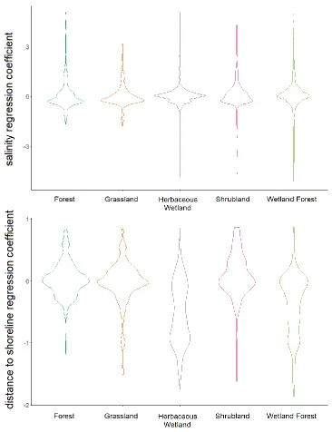
Figure 3.5 (a) GWR local R2. (b) Spatial distribution of predictor variable importance grouped into two broad categories - land use/disturbance and sea level rise explanatory variables ... 68 Figure 3.6 Maps of GWR regression coefficients for each of the predictor variables ... 69 Figure 3.7 (a) Violin plots of salinity regression coefficient across different NLCD 2001
land use and land-cover types. (b) Violin plots of distance to shoreline regression coefficient across different NLCD 2001 land use and land-cover types ... 72 Figure 3.8 Total aboveground carbon lost under inundation from the Intermediate-High
scenario (ranging from 0.3 m to 1.8 m) and predicted fractional carbon decline of remaining landscape under SLR scenarios ... 73 Figure 3.9 Fractional decline under the Intermediate-High sea level rise scenario using
GWR regression ... 74 Figure 4.1 Study area maps. (a) Southeast US with North Carolina’s Albemarle-Pamlico
Peninsula as inset map; (b) parcel typologies developed for landowner sampling stratification; (c) area of the Albemarle-Pamlico Peninsula less than 1m in elevation; (d) parcels meeting requirements for the sampling frame (e.g., privately owned, less than 1m in elevation on any portion of property, greater than 5 acres in size, and owner’s permanent residence on the APP) ... 97 Figure 4.2 Survey responses to risk perception statements, grouped by landowner
typology ... 106 Figure 4.3 Parameter estimates that have been converted to odds ratios for variables from
the survey that potentially influence behavioral intentions with respect to adaptation program enrollment. Bars are 95% confidence intervals and dots are means. Variables have been grouped into broad categories relating to different sections of the survey aimed to elicit information about landowners, information networks, and risk perception. Landscape characteristics were derived from geospatial data. ** indicates statistically significant relationship at p-value<0.05 and * indicates statistically significant relationship at
xii Figure 4.4 Heterogeneity in the random effects of landowner on model intercepts, sorted
from negative to positive ... 108 Figure 4.5 Parameter estimates converted to odds ratios from the final mixed effects
logistic regression model considering the scenario levels alone (Model 1) and considering both scenario levels and individual/property attributes (Model 2). Bars are the 95% confidence intervals and bars that do not cross the axis at one are statistically significant. ... 109 Figure 4.6 Predicted probabilities of enrollment across different payments by program
administration type for (a) agricultural landowners and (b) forest landowners, derived from a scenario based on average contract length and majority of neighbor participation ... 111 Figure 4.7 Predicted probabilities of enrollment across different contract lengths by
program administration type for (a) agricultural landowners and (b) forest landowners, derived from a scenario based on average payment and majority of neighbor participation ... 112 Figure 4.8 Predicted probabilities of enrollment across different payments based on
varying neighborhood participation levels for (a) agricultural landowners and (b) forest landowners, derived from a scenario based on average contract length and state agency program administration ... 113 Figure A.1 (a) Study area with 30 m wide transect highlighted; (b) Schematic of the
forest-transition forest-marsh vegetation gradient; (c) aerial imagery of selected 30m transect within study area that represents the forest to marsh vegetation gradient; (d) lidar point clouds of 30 m transect of vegetation gradient (top image: overhead view, bottom image: side view). ... 134 Figure A.2 A portion of the study area, showing the vegetation height difference map
between the 2001 lidar top of canopy data normalized by the 2001 lidar-derived DEM and the 2001 top of canopy data normalized by the more accurate 2014 lidar-derived DEM ... 135 Figure A.3 Kernel density estimates of lidar vegetation height distributions across the five
major study areas and vegetation communities ... 136 Figure A.4 Partial dependence plots showing relationships between the predictor variables
from the 2001 final integrated model and total aboveground biomass. Fifty percent confidence intervals are shown in grey ... 137 Figure A.5 Partial dependence plots showing relationships between the predictor variables
xiii Figure A.6 Partial dependence plots of the top three predictor variables and their
relationship with vegetation classes for the 2001 vegetation classification ... 139 Figure A.7 Permuted variable contributions toward the classification of each vegetation
type for the 2001 Random Forest classification model. Black color indicates statistically significant predictors (grey color indicates predictor is not statistically significant). X-axis represents mean decrease in accuracy ... 140 Figure A.8 Partial dependence plots of the top three predictor variables and their
relationship with vegetation classes for the 2014 vegetation classification. ... 141 Figure A.9 Permuted variable contributions toward the classification of each vegetation
type for the 2014 Random Forest classification model. Black color indicates statistically significant predictors (grey color indicates predictor is not statistically significant). X-axis represents mean decrease in accuracy. ... 142 Figure B.1 Map showing spatial autocorrelation in the residuals from the ordinary least
squares global regression model. ... 143 Figure B.2 Scaled predictor variables selected for use in the ordinary least squares global
1 CHAPTER 1
INTRODUCTION
1.1. INTRODUCTION
2 Driven by global climate change, sea level rise is already transforming coastal landscapes. We will continue to see unprecedented negative impacts from sea level rise in the coming decades. Since the 1900s, global mean sea level (GMSL) has risen by about 16 – 21 cm, with about 7 cm of rise occurring just since 1993 (Kopp et al., 2016). It is likely that we can expect a 9 – 18 cm rise in sea level by 2030, with 15 – 38 cm by 2050, and 30 – 130 cm by 2100 (Kopp et al., 2014). Some predictions even suggest that a rise of 2.4 m is plausible by 2100 (citation). The exact measures of mean sea level rise is highly regional in nature, with certain regions expected to experience higher than global average rise in sea level. One example is the Southeast U.S., which is expected to experience a rise in sea level greater than the global average because of subsidence, water groundwater water withdrawals, and its low topographic relief. Corroborating the highly regionalized nature of the extent and severity of sea level rise impacts, a recent study that linked population growth with sea level rise inundation scenarios, indicated that inundation from a 1.8 m rise in sea level by 2100 would threaten approximately 13.1 million people; 70% of whom were located within the Southeastern United States alone (Hauer et al., 2016). In addition to direct inundation from sea level rise, coastal flooding and saltwater exposure are increasingly common occurrences in coastal areas, imparting negative impacts by altering biogeochemistry and vegetation composition, causing shoreline erosion, and further exacerbating storm surge and flooding events. As sea levels rise, the landward reach of impacted areas moves further inland, increasing the areal extent of land affected, increasing the number of communities and habitats at risk (Poulter & Halpin, 2008; Church et al., 2013).
3 The resilience and adaptive capacities of these tightly coupled socio-ecological systems are partially a product of social interactions and existing governance systems – dynamic social processes that are often overlooked in climate adaptation science and policy (Koontz et al., 2015). Adaptation, as defined, is a modification of human or natural systems that allows the system to moderate new threats and also benefit from new opportunities (McCarthy, 2001). Adaptation is a socio-cognitive process that is not only comprised of adaptive behaviors but also the ever-evolving perceptions of risk, which are influenced by a range of objective and subjective factors (Grothmann & Patt, 2005; van Duinen et al., 2014). Adaptation is a particularly complex issue because it requires individuals to implement measures for which they have no past experiences or prescribed routines. Additionally, synergies and trade-offs exist between adaptation activities that modify the land and the continued production of ecosystem services (Verburg, 2004). For example, restoring a forested wetland to serve as a storm buffer also sequesters carbon, provides wildlife habitat, and improves biodiversity. Thus, adaptation has the potential to provide dual benefits – protection from climate-related risks and also the provision of additional ecosystem goods and services. For these reasons, it’s critical to understand the interactions and feedbacks between sea level rise, land-use modifications, and adaptive decision-making.
The focus of this dissertation is the exploration of linkages between spatial patterns of land change and the social processes driving the change in a tightly coupled socio-ecological system experiencing sea level rise. In this dissertation, I identified three research questions which subsequently framed the three chapters in the dissertation. These are:
RQ1: What are the spatial patterns of vegetation change in a low-lying coastal landscape vulnerable to sea level rise and salinization impacts;
RQ2: What are the relative contributions of land use- and sea level rise-drivers to the spatial patterns of vegetation change; and
RQ3: What socio-spatial factors drive landowners’ adaptive behaviors?
5
6 1.2. REFERENCES
Castella, J.C., Kam, S.P., Quang, D.D., Verburg, P.H. and Hoanh, C.T., 2007. Combining top down and bottom-up modelling approaches of land use/cover change to support public policies: Application to sustainable management of natural resources in northern Vietnam. Land use policy, 24(3), pp.531-545.
Castella, J.C. and Verburg, P.H., 2007. Combination of process-oriented and pattern-oriented models of land-use change in a mountain area of Vietnam. Ecological modelling, 202 (3-4), pp.410-420.
Church, J.A., Clark, P.U., Cazenave, A., Gregory, J.M., Jevrejeva, S., Levermann, A., Merrifield, M.A., Milne, G.A., Nerem, R.S., Nunn, P.D. and Payne, A.J., 2013. Sea level rise by 2100. Science, 342(6165), pp.1445-1445.
Duinen, R.V., Filatova, T., Geurts, P. and Veen, A.V.D., 2015. Empirical analysis of farmers' drought risk perception: Objective factors, personal circumstances, and social
influence. Risk analysis, 35(4), pp.741-755.
Filatova, T., Verburg, P.H., Parker, D.C. and Stannard, C.A., 2013. Spatial agent-based models for socio-ecological systems: Challenges and prospects. Environmental modelling & software, 45, pp.1-7.
Grothmann, T. and Patt, A., 2005. Adaptive capacity and human cognition: the process of individual adaptation to climate change. Global Environmental Change, 15(3), pp.199-213.
Hauer, M.E., Evans, J.M. and Mishra, D.R., 2016. Millions projected to be at risk from sea-level rise in the continental United States. Nature Climate Change, 6(7), p.691.
Koontz, T.M., Gupta, D., Mudliar, P. and Ranjan, P., 2015. Adaptive institutions in social ecological systems governance: A synthesis framework. Environmental Science & Policy, 53, pp.139-151.
Kopp, R.E., Horton, R.M., Little, C.M., Mitrovica, J.X., Oppenheimer, M., Rasmussen, D.J.,
Strauss, B.H. and Tebaldi, C., 2014. Probabilistic 21st and 22nd century sea‐level projections at a global network of tide‐gauge sites. Earth's Future, 2(8), pp.383-406.
7
Mitrovica, J.X., Morrow, E.D. and Rahmstorf, S., 2016. Temperature-driven global sea-level variability in the Common Era. Proceedings of the National Academy of Sciences, p.201517056.
Liu, J., Dietz, T., Carpenter, S.R., Alberti, M., Folke, C., Moran, E., Pell, A.N., Deadman, P., Kratz, T., Lubchenco, J. and Ostrom, E., 2007. Complexity of coupled human and natural systems. Science, 317(5844), pp.1513-1516.
Liu, J., Hull, V., Batistella, M., DeFries, R., Dietz, T., Fu, F., Hertel, T.W., Izaurralde, R.C., Lambin, E.F., Li, S. and Martinelli, L.A., 2013. Framing sustainability in a telecoupled
world. Ecology and Society, 18(2).
McCarthy, J. J., Canziani, O. F., Leary, N. A., Dokken, D. J., & White, K. S. (Eds.).
(2001). Climate change 2001: impacts, adaptation, and vulnerability: contribution of Working Group II to the third assessment report of the Intergovernmental Panel on Climate Change (Vol. 2). Cambridge University Press.
Parker, D.C., Manson, S.M., Janssen, M.A., Hoffmann, M.J. and Deadman, P., 2003. Multi- agent systems for the simulation of land-use and land-cover change: a review. Annals of the association of American Geographers, 93(2), pp.314-337.
Poulter, B. and Halpin, P.N., 2008. Raster modelling of coastal flooding from sea‐level
rise. International Journal of Geographical Information Science, 22(2), pp.167-182. Rounsevell, M.D.A., Arneth, A., Alexander, P., Brown, D.G., de Noblet-Ducoudré, N., Ellis, E.,
Finnigan, J., Galvin, K., Grigg, N., Harman, I. and Lennox, J., 2014. Towards decision-based global land use models for improved understanding of the Earth system. Earth System Dynamics, 5(1), pp.117-137.
8 CHAPTER 2
COASTAL BIOMASS LOSS FROM SEA LEVEL RISE
QUANTIFIED WITH REPEAT LIDAR SURVEYS
2.1. INTRODUCTION
Though coastal forests comprise a small fraction of the Earth’s surface, they play an important role in global carbon storage and sequestration (Mcleod et al., 2011; Krauss et al., 2018). Due to human population growth, amenity-migration to coastal regions, and unsustainable land-use practices, these areas are experiencing alarming and unprecedented declines (Weng, 2002; Thomas et al., 2017). Compounding these stressors are additional factors related to climate change – particularly direct inundation from sea level rise and saltwater intrusion (Young, 1995; Hackney and Yelverton, 1990; Pearsall and Poulter, 2005; Herbert et al., 2015). The accelerating rate of sea level rise is anticipated to have a significant impact on coastal forests throughout the 21st Century
(i.e., Hauer et al., 2016; Karegar et al., 2016). As the landward extent of sea level rise impacts moves further inland, inundation, flooding, erosion, and saltwater intrusion will become increasingly common occurrences in coastal forests (Hauer et al., 2016; Nicholls & Cazenave, 2010). More salt-tolerant vegetation will begin to encroach into coastal forests as salinity intrudes and sea levels rise, reducing their extent and impacting the continued ability of coastal forests to serve as carbon sinks. The uncertain future makes it difficult to develop sound land-use management practices and policies to mitigate coastal forest decline. This highlights the growing need for rigorous studies of how land- and climate-change will affect coastal ecosystem function, carbon pools, and overall contributions to the global carbon budget. Consequently, methods to measure and monitor these vegetation responses are crucial for understanding the continued persistence of the coastal ecosystem services upon which human health and well-being depend.
9 data collection often limits practical use of field measurements of aboveground biomass (AGB) over large extents, especially for repeat and accurate measurements through time. Thus, analyses of landscape-scale processes warrant a combination of ground-based measures of change and remote sensing technologies. The use of remote sensing data in aboveground biomass estimation, with its broad coverage and moderate-to-high spectral, spatial and temporal resolutions has become an important field of research in recent years (Fatoyinbo et al., 2018). AGB has been successfully estimated using derived metrics from multi-spectral satellite imagery in correlative models linking these metrics with field data (DeFries et al., 2002; Kulawardhana et al., 2014; Lefsky et al., 2002). Particularly useful metrics for AGB estimation are derived vegetation indices like the normalized difference vegetation index (NDVI) and the enhanced vegetation index (EVI; Hardisky et al., 1986; Ramsey et al., 2014). Because of its predictive power, multi-spectral satellite imagery has become a common source for biomass estimation at regional scales as has the use of time-series satellite imagery to evaluate biomass dynamics (Klemas, 2001; Byrd et al., 2014; Pflugmacher et al., 2014). However, mixed pixels and data saturation often reduce accuracy in complex biophysical environments (Byrd et al., 2014; Lu, 2006).
10 studies have evaluated the utility of integrating repeat lidar data and satellite imagery to quantify aboveground biomass dynamics in such varied environments. Thus, the applicability of repeat lidar and multi-spectral data integration in coastal environments remains promising, although as of yet, largely unexplored.
Rapid advancements in these remote sensing technologies require the development of methods to reconcile datasets with disparate resolutions and different data collection specifications. Analyses predicting biomass change using repeat lidar datasets, generally apply two main approaches for modeling AGB – direct and indirect. Direct approaches calculate biomass change based on the differences in lidar measurements from different time periods, whereas indirect approaches model biomass for each time period and then calculate the difference (Cao et al., 2016). Studies comparing the success of the two approaches have been mixed, with some suggesting that the direct approach provides much more accurate biomass estimates and change over time (Cao et al., 2016; Næsset et al., 2013) and others favoring the indirect approach; which has had particular success in young or managed forests (Hudak et al., 2012; Økseter et al., 2015). Despite methodological developments in lidar data processing and repeat data interpretation, a research gap exists integrating disparate multi-temporal remote sensing data sources along with the above-mentioned methods to measure AGB changes across large geographic extents composed of highly varied vegetation.
11 highly heterogeneous coastal environment. Results from this research have the ability to directly inform management- and policy-related research related to global change and climate adaptation.
2.2. METHODS
We estimated biomass change from 2001 to 2014 using field measurements, Landsat and lidar datasets. We used the Random Forest algorithm (RF) to model changes in AGB across the study area. We employed (1) a direct approach where biomass change is calculated as the difference between the remote sensing metrics; and (2) an indirect approach where biomass is modeled for each point in time and then differenced to create biomass change. We predicted vegetation types at each time step using RF and then performed a change analysis using the two resultant maps. We evaluated the performance of model accuracies and assessed the accuracy gained by incorporating independent remote sensing data.
2.2.1. Study system
The Albemarle-Pamlico Peninsula in eastern North Carolina, USA, is an approximately 6,600-km2 coastal region buffered from the Atlantic Ocean by a change of barrier islands and the Albemarle-Pamlico Estuary. Situated within the North American Coastal Plain, which has some of the highest biodiversity in all of North America, the Albemarle-Pamlico Peninsula has many unique natural ecosystems (Noss et al., 2015). Of particular ecological importance are the many peatland pocosins, the wet longleaf pine savannas, and freshwater forested wetlands which comprise more than 50 percent of the peninsula and the more than 15 tree species that characterize these ecological systems. Aside from wetlands, the peninsula supports forestry and agricultural operations along with many private and public land inholdings interspersed. While the peninsula provides significant ecosystem services, such as wildlife habitat, carbon sequestration and storm surge protection, over half of this landscape is below 1-m in elevation making it highly vulnerable to sea level rise.
12 ecosystems common in the study area. Although tolerant of brief saltwater intrusion events, prolonged or extreme saltwater exposure in upland forests results in a gradual shift towards that of brackish or saline marsh characteristics of herbaceous plants like sawgrass (Cladium jamaicense) and black needlerush (Juncus romerianus) (Moorhead & Brinson, 1995; Poulter et al., 2009). This prevents regeneration as seedlings aren’t as tolerant to salinization events and also leads to die-off of mature trees, leaving stands of dead trees known as ‘ghost forests’. As saltwater intrusion and flooding become more frequent and severe, coastal forests gradually transition from multi-layered and structurally complex communities to herbaceous wetlands with little vertical complexity as more salt-tolerant species move into these areas once the canopy opens. A narrow transition zone marked by dead trees, salt-tolerant shrubs, and herbaceous ground cover typically lies in between these two zones.
2.2.2. Field data collection
We selected five sites to conduct field surveys along the shoreline of the Albemarle-Pamlico Peninsula that were accessible by road, under 1-m elevation, and publicly owned. To evenly distribute sampling locations across the forest-marsh interface, we delineated three vegetation zones at each site (forest, transition, and marsh), and randomly selected 7, 12-m radius vegetation plots in each zone (Figure 2.1). At one site, Palmetto Peartree, there was no marsh zone so we only established 14 plots, as opposed to the 21 plots established at the remaining 4 sites. We ensured each plot was 20 m away from the zone boundary and at least 60 m from any other plot center. We first inventoried vegetation between November 2003 and February of 2004, and then revisited the plots between April and July 2016 using the same protocol. We recorded species name, diameter at breast height (dbh) and height for live woody species greater than 2.5 cm in diameter at each plot. For vegetation less than 1-m in height, we recorded percent cover within five 1-m2 subplots and obtained an average cover value for each species at each plot by averaging
13
Figure 2.1: The Albemarle-Pamlico Peninsula is located in eastern North Carolina of the United States. Ninety-eight random field plots were established across five sites (with 21 plots in each site except for Palmetto Peartree, which lacked marsh communities) among three vegetation communities: forest, transition forest, and marsh.
Table 2.1: Allometric biomass equations for woody and herbaceous vegetation.
(a) WOODY & SHRUB (>2.5cm); field measure: basal diameter; sources: Jenkins et al., 2003 and Smith and Brand, 1983
β0 β1 Category Obs r2
pine* –2.5356 2.4349 softwood 180 0.98
softwood (dead stem wood)† -0.3737 -1.8055 softwood 781 0.15 cedar (juniperus)* –2.0336 2.2592 softwood 250 0.98 soft maple (red maple)* –1.9123 2.3651 hardwood 316 0.95 mixed hardwoods* –2.4800 2.4835 hardwood 289 0.98 hardwood (dead stem wood)† -0.3065 -5.424 hardwood 264 0.24 Myrica pensylvanica‡ 60.795 2.867 shrubs (>2.5cm) 20 0.98
(b) HERBACEOUS & SHRUB (<2.5cm); field measure: percent cover; source: Smith and Brand, 1983
A B Category Obs r2
14
Table 2.1: Continued.
Rubus pubescens‡ 0.0214 1.6346 vines 168 0.78
Aster ‡ 0.1192 1.0226 forbs 344 0.50
vaccinium angustifolium ‡ 0.1496 1.2458 shrubs (< 2.5cm) 104 0.72
Pteridium aquilinum‡ 0.459 0.7669 ferns 15 0.50
* bm=Exp(β0 + β1lndbh), unit:kilograms † ratio=Exp(β0 + β1/dbh), unit:ratio
‡ bm= aXb, unit: grams
2.2.3. Lidar data processing
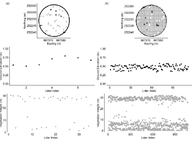
We obtained lidar datasets for 2001 and 2014 for the entire study area from the NOAA Coastal Services Center (2001 data; https://coast.noaa.gov/digitalcoast/) and the US Fish and Wildlife Service and US Geological Survey (2014 data; Doug Newcomb, US FWS). The average point density was 0.11/m2 for the 2001 LiDAR data 2.0/m2 for the 2014 lidar data (Figure 2.2, Figure A.1).
Figure 2.2: An example 450m2 forested field plot in the Palmetto Peartree study area, showing the difference in
15 See Table 2.2 for flight specifications, densities, and vertical accuracies. A classification was provided for the 2014 lidar point cloud so this was used to differentiate the lidar returns. We used the multiscale curvature classification (MCC) algorithm to classify the 2001 lidar data into ground and vegetation types (Evans & Hudak, 2007). We used the average post spacing and a curvature threshold appropriate for the dominant vegetation in the study area, to adjust the scale parameters of the MCC algorithm (Tinkham. et al., 2012). We applied a regularized spline with tension method to interpolate digital elevation models (DEM) from the ground points at 3-m resolution for each period followed by a spline smoothing algorithm to remove noise (Mitasova et al., 2005). To ensure consistency between these two lidar datasets, we checked for systematic errors by comparing derived DEMs along permanent features with geodetic benchmarks found in the study area.
Table 2.2: Acquisition parameters for lidar surveys in 2001 and 2014. Lidar data collected as part of the North Carolina Floodplain Mapping Program.
2.2.4. Lidar Vegetation Metrics
We estimated vegetation height by subtracting the high resolution DEMs derived for each year from each year’s associated lidar point cloud data classified as vegetation. We generated landscape-scale vegetation height and density metrics across the entire study area using 12-m resolution grids, by binning the vegetation height points at the specified resolution and performing the appropriate univariate statistics (Table 2.3). Metrics most closely related to vegetation structural components and commonly used in other lidar vegetation studies were selected for inclusion in this study (Lefsky et al., 2001; Sexton et al., 2009; Singh et al., 2016; Smart et al., 2012). Detailed descriptions of each of the metrics can be found in Table 3. Vegetation heights were also binned into height strata by applying height thresholds associated with vegetation understory, midstory, and overstory. The 12-m resolution was selected to ensure sufficient lidar data in each grid cell for 2001 while retaining some of the detailed information available with the
Survey Date Altitude Multiple Returns
Swath Width
Scan Angle
RMSEz Average Post Spacing
Average Point Density Jan-March 2001 3,658 m 5 returns per
pulse
3,411 m 25° 0.2 m 3 m
0.11/m
2
January 2014 1676 m 4 returns per pulse
1,025 m 34° 0.17 m 0.7 m
2.0/m
16 2014 data. Later, we resampled these and the DEMs to 30 m using the bilinear resampling method to match the spatial resolution of Landsat imagery. The different spatial resolutions were then used to explore the effect of scale on total AGB predictions. We used invariant features such as road centerlines and parking lots as reference points to ensure alignment between the Landsat imagery and lidar-derived vegetation metrics. In the end, we had sets of vegetation metrics for 2001 and 2014 at both 12-m and 30-m resolution for each year.
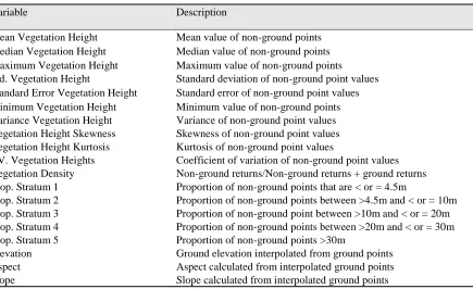
Table 2.3: Predictor variables derived from lidar data by binning the appropriate statistics at selected grid resolution (e.g. 12-m resolution as in this analysis).
Due to the 18-fold difference in lidar point densities, three measures of vegetation structure collected in the field (mean, maximum, and standard deviation) were compared to the lidar-derived canopy height variables. Plotting the density distributions of field and lidar data for maximum and mean vegetation height, we notice a visible shift toward the origin – a shift that is apparent in both the field data and the lidar data (Figure 2.3).Though the shift is apparent in both the lidar and field data, the lidar distributions of maximum and mean height don’t align exactly with the field data in either year. Both lidar surveys underestimated mean vegetation height, a common phenomenon previously reported in lidar studies (Lim et al., 2003) but linear relationships between the field and lidar data were moderate to strong (R2adj=0.4 for 2001 and R2adj=0.53 for 2014). Maximum height
was underestimated in 2001 and slightly overestimated in 2014 (Table 2.4). An additional accuracy
Variable Description
Mean Vegetation Height Mean value of non-ground points Median Vegetation Height Median value of non-ground points Maximum Vegetation Height Maximum value of non-ground points Std. Vegetation Height Standard deviation of non-ground point values Standard Error Vegetation Height Standard error of non-ground point values Minimum Vegetation Height Minimum value of non-ground points Variance Vegetation Height Variance of non-ground point values Vegetation Height Skewness Skewness of non-ground point values Vegetation Height Kurtosis Kurtosis of non-ground point values
CV. Vegetation Heights Coefficient of variation of non-ground point values Vegetation Density Non-ground returns/Non-ground returns + ground returns Prop. Stratum 1 Proportion of non-ground points that are < or = 4.5m
Prop. Stratum 2 Proportion of non-ground points between >4.5m and < or = 10m Prop. Stratum 3 Proportion of non-ground point between >10m and < or = 20m Prop. Stratum 4 Proportion of non-ground points between >20m and < or = 30m Prop. Stratum 5 Proportion of non-ground points >30m
17 check of the different DEMs used to generate the height metrics was performed and a comparison was made between the 2001 lidar vegetation height normalized by the 2001 DEM and the 2014 DEM. Statistical comparisons showed no significant difference, with a mean difference of only 0.02 m in height with a 1.2-m standard deviation across the entire study area (Figure A.2). Because the magnitude and direction of the lidar data shifts were similar, we made the decision not to perform a linear bias correction (normalizing the 2001 data by 2014 data).
Figure 2.3: Comparison of field data and lidar data kernel density distributions for maximum vegetation height and mean vegetation height at the 98 study site plots.
Table 2.4: Summary statistics of field and lidar data for plots across the three vegetation communities in 2001 and 2014. All values are in meters.
Marsh (n=28) Transition Forest (n=35) Forest (n=35)
Mean Max. Std. Dev. Mean Max. Std. Dev. Mean Max. Std. Dev.
2001
Field height 0.0 0.0 0.0 4.2 6.0 1.5 9.8 17.8 4.2 Lidar height 0.6 1.1 0.3 2.6 9.3 3.4 7.4 15.5 5.5
2014
Field height 0.1 0.1 0.0 1.9 3.6 0.6 4.9 11.9 2.6
18 2.2.5. Landsat data processing
We collected Landsat 7 ETM+ and Landsat 8 OLI images at path 14 and row 35 for 2001 and 2014 from the USGS data portal (http://glovis.usgs.gov). We obtained cloud free images on or near the lidar flight dates and field survey seasons to maximize comparability, and examined the Palmer Drought Severity Index (PDSI) to confirm that the images were not from extreme dry years (Table 2.5). We calculated indices, such as tasseled cap brightness, greenness, wetness, tasseled cap wetness-greenness difference, normalized difference vegetation index (NDVI), and the enhanced vegetation index (EVI). To measure spectral signatures during periods of peak biomass, we obtained mid-summer NDVI and EVI images for 2001 and 2014 from Google Earth Engine (mean and maximum NDVI and EVI across cloudless portions of all 32-day composites from May to August; https://earthengine.google.com/). We used combinations of these indices in addition to the six spectral Landsat bands in the Random Forest models (Table 2.6).
Table 2.5: Specifications of Landsat imagery for 2001 and 2014 along with Palmer Drought Severity Index (PDSI) for relative dryness that ranges from -10 (dry) to 10 (wet).
Date Source Cloud Cover (%) Precipitation (in) PDSI*
2000/11/28 Landsat 7 ETM+ 0.00 3.2 -0.64
2013/11/24 Landsat 8 OLI 0.10 3.59 0.9
2001/04/05 Landsat ETM+ 0.00 1.85 -1.69
2014/04/01 Landsat 8 OLI 36.43 4.73 1.61
Table 2.6: Metrics derived from spectral bands of Landsat data. Spectral Index Description
NDVI Normalized difference vegetation index
Average NDVI Average NDVI value of pixels from cloudless portions of all 32-day composites from May through August for 2001 and 2014
Maximum NDVI
Maximum NDVI value of pixels from cloudless portions of all 32-day composites from May through August for 2001 and 2014
EVI Enhanced vegetation index
Average EVI Average EVI value of pixels from cloudless portions of all 32-day composites from May through August for 2001 and 2014
Maximum EVI Maximum EVI values of pixels from cloudless portions of all 32-day composites from May through August for 2001 and 2014
TCW Tasseled cap wetness index TCB Tasseled cap brightness index TCGRN Tasseled cap greenness index
TCWGD Difference between TCW and TCGRN
19
Table 2.6: Continued.
Green Band Band 2 in Landsat 7ETM+; Band 3 in Landsat 8OLI
NIR Band Near infrared; Band 4 in Landsat 7ETM+; Band 5 in Landsat 8OLI SWIR Band Short wave infrared; Band 7 in Landsat 7ETM+; Band 7 in Landsat 8OLI
2.2.6. Predictive modeling
We used Random Forest (RF) to predict spatial and temporal changes in biomass. RF is an ensemble learning method for classification and regression that functions by constructing many decision trees for model training and then generating mean predictions or the mode of classes across the individual trees (Breiman, 2001; R statistical software package ‘randomForests’; R Core Development Team, 2018). The algorithm corrects for decision trees’ tendency of overfitting their training datasets through its bootstrap approach. We used the derived relationship between field biomass, Landsat data, and lidar data at the field training plots to predict total aboveground biomass for all other pixels at 12-m and 30-m resolution.
To evaluate biomass change during the study period, we took two different approaches. First we used a direct approach by predicting biomass change directly using the differences in biomass estimated from the field-data and the differences in the remote sensing metrics between the two time steps. We then applied an indirect approach where we treated 2001 and 2014 as separate assessments and developed predictive biomass models separately but consistently for each time period (following Hudak et al., 2012). The indirect modeling approach was used to develop four model sets: (1) a 12-m lidar only model; (2) a 30-m lidar only model; (3) a 30-m Landsat only model; and (4) a 30-m lidar and Landsat integrated model (referred to as the 30-m resolution integrated model). We used the Model Improvement Ratio (MIR) function to select the best predictor variables among the suite of candidate variables (Table 2.3, Table 2.6). If selected predictor variables were highly correlated (r>0.9), we excluded the variable with the lower MIR value, re-ran the model selection function and re-evaluated the outputs (Hudak et al., 2012). We repeated these steps until we selected the most parsimonious model with the highest R2 and lowest
multicollinearity among predictor variables.
20 cells across the study area for 2001 and 2014 at 30-m resolution. To develop the most parsimonious model, we selected the predictor variables using the same methods we used for the biomass models. We performed a change analysis on these two classifications so that changes in imputed biomass could be mapped to changes in these vegetation types.
2.2.7. Evaluation of model performance
Because of the limited number of reference plots, we used all of the field data collected in 2003 and 2016 to train the RF models. For time one, we used the 2003 field plots to train the 2001 biomass model and for time two, we used the 2016 field plots to train the 2014 biomass model. We used a bootstrap approach to provide an independent assessment of model performance for validation. Using 1,000 permutations of the fitted RF model, we first tested model significance and then performed a 100-fold cross-validation withholding 10% of the data each time for validation and running the model on the subset data. Permutation tests of significance and cross-validation were performed using the package ‘rfUtilities’ and ‘rfPermute’ in R (Evans and Murphy, 2018; R Core Development Team, 2018). We explored the linear relationship between biomass change measured at the field plots and predicted change from the RF models. To summarize changes in biomass and vegetation types across the natural landscape, we used a systematic sample of the landscape at 500-m intervals. We removed any portion of the landscape that was designated as cropland or developed, and finally, matched the study area extent to avoid discrepancies in summaries due to land loss from erosion and sea level rise. We also removed from the summaries, those areas that experienced biomass changes due to fire.
2.3. RESULTS
2.3.1. Plot level estimates of biomass change
From the field data, we observed a significant decrease in AGB between 2003, referred to as T1, and 2016, referred to as T2 (mean= -8.8 Mgha-1 and p-value= 0. 03, Figure 2.4) at the plot
scale. Plots classified as forest showed significant decline in mean AGB of 19.2 Mgha-1 (28%
21 decrease (36% decrease) in AGB, and although small, it was significant (T1= 0.5 Mgha-1, T2= 0.3 Mgha-1, p-value= 0.05).
Figure 2.4: Mean field-measured aboveground biomass by community type and year. The * denotes a statistically significant difference between years (p<0.05).
2.3.2 Predictive model performance
We mapped biomass change directly using field-measured change in AGB as the response variable along with 2001-2014 change maps of the suite of predictor variables. Overall model performance was poor and imputed AGB change for the majority of the landscape was negative with a mean biomass change of -10.7 Mgha-1 (cv- R2adj.= 0.37; RMSE= 15.9, 15.6%). There was a
22 We tested the fitted model significance against random and found that both the 2001 and 2014 fitted models were statistically significant at the 0.001 level. Among indirect models, the 2014 12-m resolution model performed the best with R2adj. of 0.84 and RMSE of 7.8% compared
to the 2001 12-m model with R2adj. of 0.50 and RMSE of 17.7%. The 2001, 30-m resolution lidar
only model performed moderately well at R2
adj. of 0.66 and RMSE of 15.7%. The 2014, 30-m
resolution lidar only model performed only slightly worse than its 2014 30-m resolution integrated final model counterpart with R2
adj. of 0.76 and RMSE of 9.6%.
When considering both time steps, the 30-m resolution integrated models performed the best with R2adj. of 0.75 (RMSE= 12.6%) for 2001 and R2 adj. of 0.78 (RMSE= 9.5%) for 2014
(Figure 2.5). In 2001, mean AGB measured 52.5 Mgha-1 with a standard deviation of 30.4 Mgha-1 (cv-Radj.2= 0.75; cv-RMSE= 18.3 Mgha-1, 12.6%). Mean AGB for the 2014 model measured 60.6
Mgha-1 with a standard deviation of 40.8 Mgha-1 (cv- Radj.2= 0.78; cv-RMSE= 15.0 Mgha-1, 9.5%)
23
24
Figure 2.6: Observed biomass plotted against the Random Forest imputed biomass estimates, derived from 1,000 regression trees and separated by vegetation community type (Forest, Transition Forest, and Marsh) for (a) 2001 and (b) 2014.
We calculated the standard deviation and coefficient of variation for each pixel in the landscape for the final integrated 30-m resolution model. The standard deviation maps were similar for 2001 and 2014, with the 2001 map having slightly higher minimum (2001 minimum= 0.5 Mgha-1, 2014 minimum= 0.6 Mgha-1), higher maximum (2001 maximum= 68.8 Mgha-1, 2014 maximum= 63.4 Mgha-1), and lower mean values (2001 mean= 26.7 Mgha-1, 2014 mean= 29.1
25 the perimeter of the study area (where marsh vegetation is most common) in 2001 than in 2014. The highest variability in the 2014 map appears to occur within the fire perimeters.
26
27 2.3.3. Contribution of vegetation metrics
Using the indirect modeling approach, we mapped two independent biomass predictions and have two separate, but consistent Random Forest models for evaluation. EVI and median vegetation height were the two most important predictor variables in the 2001 final integrated 30-m 30-model. (Figure 2.8). According to partial dependence plots, there were positive relationships between EVI and AGB as well as median height and AGB (Figure A.4). Mean vegetation height and variance in vegetation height were the most important predictor variables for the 2014 final integrated 30-m resolution model. According to the partial dependence plots, both predictor variables had positive relationships with AGB (Figure A.5). Additional important variables for both models were those associated with the different vegetation strata and metrics associated with canopy variation (standard deviation and variance). Although spectral indices were important for the model fit to the 2001 data, they did not provide statistically significant contributions to the overall predictive power of the model in 2014. Interestingly, the top two-predictor variables at any resolution (12-m resolution, 30-m resolution lidar only and 30-m resolution integrated) were consistent with mean or median vegetation height listed in all models (Table 2.7). The main difference between the final integrated models and the other models is the contribution of spring EVI to overall predictive power in the 2001 30-m resolution integrated model, improving the Radj.2
28
Figure 2.8: Permutation importance of predictor variables derived from 1,000 permutations of the final fitted Random Forest models for (a) 2001 and (b) 2014. Percent increase in MSE is the increase in mean square error of predictions as a result of each variable being randomly permuted. The higher the increase, the more important the variable. Black color indicates contribution is statistically significant.
29 For the 2001 vegetation imputation, the most important predictor variable across all three-vegetation classes was NDVI, followed by variance in three-vegetation heights compared to the 2014 vegetation imputation, which showed EVI, followed by maximum vegetation heights as important predictors. In 2001, the most important class-level variables for predicting the forest type included spring NDVI, Looking at the most important class-level variables for 2001, we find that spring NDVI is important for all three vegetation communities. For forests, NDVI was followed by median and variance in vegetation heights. Spring SWIR and fall Tasseled Cap Wetness Index were the next most important predictors for transition forest. For marsh, in addition to NDVI, variance in vegetation heights and fall Tasseled Cap Greenness index were most important (Figure A.6, Figure A.7). In 2014, the most important class-level variables included maximum vegetation heights, fall EVI, and variance in vegetation heights for forest. Fall SWIR, fall Tasseled Cap Wetness Greenness Difference, and variance in vegetation heights were the most important predictors for transition forest. And for marsh, maximum vegetation heights, fall EVI, and median vegetation heights were most important (Figure A.8, Figure A.9).
Table 2.7: Model performance measures and statistics for each of the tested models: 12-m resolution model with lidar data only, 30-m resolution data with lidar only, and 30-m resolution integrated model with both lidar and Landsat data.
Model
cv-Radj.2
cv-RMSE (Mgha-1)
Top Predictor Variables*
Min (Mgha-1)
Max (Mgha-1)
Mean (Mgha-1)
Standard Deviation (Mgha-1)
2001 12-m Lidar
0.50 25.0 (17.8%)
Mean Height; Median Height
1.0 141.6 37.9 32.5
2014 12-m Lidar
0.84 12.2 (7.8%)
Mean Height; Variance Height
1.0 157.7 57.0 39.6
2001 30-m Lidar
0.66 22.4 (15.7%)
Median Height; Prop. Stratum 2
1.3 143.6 36.4 28.4
2014 30-m Lidar
0.76 15.5 (9.6%)
Mean Height; Variance Height
0.7 162.8 58.6 40.6
2001 30-m Landsat
0.69 20.9 (14.0%)
Spring EVI; Fall SWIR
0.6 145.9 65.3 44.1
2014 30-m Landsat
0.44 21.9 (16.5%)
Fall NDVI; Fall NIR
0.5 132.3 47.8 29.4
2001 30-m Integrated
0.75 18.3 (12.6%)
Spring EVI; Median Height
0.4 145.6 52.5 30.4
2014 30-m Integrated
0.78 15.0 (9.5%)
Mean Height; Variance Height
0.5 158.7 60.6 40.8
* Top two predictor variables contributing significantly to overall model predictive power as measured by percent
30 2.3.4. Coastal forest declines and aboveground biomass change
31
32 Using our change analysis of vegetation types, we showed that 73% of the study area did not experience a change in vegetation type (Figure 2.10). Forested areas that remained forested throughout the study period experienced an overall net AGB gain of 7.9 Mgha-1 (Figure 2.11). Areas experiencing coastal forest declines, or a change from forest to transition forest comprised 18% of the landscape and showed an overall decrease in biomass of 31.2 Mgha-1. Areas changing
from transition forest to marsh comprised only 1% of the landscape but showed a decrease in biomass of 15.6 Mgha-1. Both transition forest and marsh that remained static throughout the study
period still exhibited overall net declines in AGB (-2.5 Mgha-1 and -6.6 Mgha-1, respectively).
33
Figure 2.11: Relationship between aboveground biomass change and vegetation classification change between 2001 and 2014. Mean AGB change was sampled using a systematic grid of points with a minimum distance between points of 500 m. Croplands, fires, and developed areas were excluded from the estimates. On the secondary axis is mean distance to the estuarine shoreline (km) for each class. Area (km2) and percent of natural landscape for each
transition type are included under each class transition.
The relationships between all change models and the change measured in the field were strong (Figure 2.12). The strongest relationship between the field data and the imputed models was found for the 30-m resolution integrated model (Radj.2=0.63, RMSE=9.1%), followed by the 12-m
resolution model (Radj.2=0.61, RMSE=9.5%), the 30-m resolution LiDAR only model (Radj.2=0.58,
RMSE=10.2%), and lastly the Landsat only model (Radj.2=0. 1, RMSE=14.0%). All three models
for the indirect modeling approach provided an increase in Radj.2 and lower RMSE values compared
to the modeled output for the direct modeling approach (Radj.2=0.37, RMSE=15.7%). Not only
34
Figure 2.12: Relationship between field biomass change between 2001 and 2014 at the plots and predicted biomass change from (a) the 12-m resolution models; (b) the 30-m resolution lidar only models; (c) the 30-m resolution Landsat only models; and (d) 30-m resolution integrated models.
2.4. DISCUSSION
This study evaluated multi-sensor remote sensing data integration to predict AGB change across a vegetation gradient in a coastal ecosystem. Coastal vegetation dynamics are highly complex and are the result of a range of natural and anthropogenic disturbances, of which, a portion of these changes in biomass likely result from the negative consequences of sea level rise. In previous studies linking lidar data to biomass change in temperate forests, results generally indicated increasing trends in biomass (e.g. from natural forest succession) or decreasing trends related to forest management (e.g. harvesting) (Hudak et al., 2012; Cao et al., 2016; Naesset et al., 2011). The integration of multi-spectral satellite imagery and lidar data in this study showed an overall decreasing trend in biomass across the study area.
35 plantations showed AGB increases (2.9 Mgha-1y-1) similar to the IPCC-reported annual accumulation of biomass in temperate loblolly plantation, which is listed as 4.0 Mgha-1y-1, but can vary by the age and other characteristics of the plantation (IPCC, 1996). Our study results showed a net loss of 0.9 Mgha-1 in aboveground biomass AGB over a 13-year time period in a dynamic coastal environment. The yearly value of carbon lost from this is equivalent to losing the carbon sequestration capacity of 220 km2 of forest a year or releasing greenhouse gas emissions from 9,902 passenger vehicles driven in a year (epa.gov).
Spatial extrapolation of biomass across the study area revealed carbon dynamics related to disturbance regimes that can act to either exacerbate or mitigate climate change effects. The spatial extrapolation revealed the effects of several fires in the study area that occurred during the 13-year period. High-intensity fire is the predominant disturbance in southeastern USA sawgrass and pine wetlands (Poulter et al., 2009b). Two large fires occurred between 2001 and 2014. The fire perimeters were confirmed using a vector shapefile available from the Monitoring Trends in Burn Severity Program (MTBS; https://www.mtbs.gov/). In 2008, the Evans Road fire burned in the central portion of the study area, south of Phelps Lake. The fire covered an area of 165.5km2 and resulted in an overall mean biomass decrease across the study period of 32.5 Mgha-1. In 2011, the Pains Bay fire burned approximately 151.6km2 in the eastern portion of the study area within the Alligator National Wildlife Refuge. Again, overall biomass decreased by 30.9 Mgha-1 at the end of the study timeframe. Although, there is regeneration within the fire perimeters as evidenced by some positive biomass change values, the overall mean remains negative.
Quantifying the impacts of fire on carbon dynamics throughout the region is important. As demonstrated here, a large contributor to the changes in aboveground biomass were the large wildfires in the study area. Given the typical fire return intervals for this region (Frost, 1995) and the study time frame, we would expect that the regeneration from these disturbances would offset much of the loss in AGB which is not what we have shown here. It’s possible that as sea level continues to rise, the interaction between fire and salinization or inundation, could alter successional pathways post-fire. Despite the historic role of fire in maintaining vegetation structure and composition in this region, the effects of fire may change along with changing climate.
36 Kirwin and Megonigal, 2013; Krauss et al., 2018). We corroborated the likely transition events by intersecting the derived land cover change maps with the AGB change maps. With this intersection, we showed areas of within-type AGB variability that could represent the leading edge of the transition process. This is important and may have otherwise gone unquantified if we were to use common land-use and land cover change-driven carbon models (Brown, 2002; Houghton, 2005). For vegetation types that showed no change throughout the study period, we showed there were at times significant changes in AGB for these types. For example, we observed a net AGB decrease within the transition forest-type extent that remained transition throughout the 13-year study period. This could suggest that some of these transition forests are moving toward a more marsh-like vegetation community, although they have not yet reached this new state (Brinson et al., 1995; Poulter et al., 2009b). The ability to identify these areas is critical because these wetlands at various stages of transition between forest and marsh represent the leading edge of climate change as salinity intrudes and sea levels rise and help us identify areas that are particularly vulnerable.
2.4.2. Multi-sensor data integration proves beneficial
Through predictive modeling and spatial mapping across a large landscape, our analysis demonstrates that an integration of lidar and Landsat satellite imagery can be highly effective at predicting biomass for multiple periods across a vegetation gradient from forest to marsh. Even at 30-m resolution, models for both 2001 and 2014 produced R2adj. values greater than 0.7, meeting
37 performance that the lidar -derived metrics did. Therefore, incorporating satellite imagery may be a way to improve the comparability of models derived for two different times with lidar surveys of varying point densities (Zolkos et al., 2013; Zald et al., 2016).
Looking at the relationship between observed and predicted biomass change, the models including only lidar data proved almost as accurate as the final integrated model. Even though the accuracies of the 2001 lidar only models were lower than the others, the mapped change from the lidar-only models showed strong relationships with actual field-based changes. In this study, despite an 18-fold difference in lidar point densities, we were able to estimate biomass with high accuracy for both the 12-m and 30-m resolution models, although aggregation to 30-m resolution made the lidar data discrepancies between years less discernible. This corroborates Hudak et al., 2012, which showed that despite large differences in lidar point densities, there was little impact on the ability to accurately map biomass change.
Landsat only models however, proved poor estimators of biomass change (R2adj. = 0.07),
although the predictive power of the independent biomass models was moderate for 2001 and 2014, with the 2001 model slightly outperforming the 2014 model. Because of the highly dynamic and varied nature of the vegetation being estimated, it’s likely that there is much more variability in the spectral signatures of the different vegetation communities than their structural characteristics. The spectral signatures can also be influenced by environmental characteristics like precipitation, cloud cover, etc. Although we did our best to account for these environmental characteristics, it is possible that the variability is too high to attempt biomass estimation from only one or two Landsat images for each year. An area of research warranting further investigation is the use of seasonal time series of satellite imagery and derived vegetation indices to estimate biomass dynamics (Zhu et al., 2015).
38 for transition forest classification in both years included spectral bands and spectral indices associated with moisture (e.g. shortwave infrared band and tasseled cap wetness index). It appears that transition forests fall between the less wet forest type and the very wet marsh type. These spectral indices may prove very useful, in conjunction with lidar, for mapping these transitions in other study areas. And as mentioned above, these transition forests have come to represent the leading edge of climate change, therefore the ability to map these areas accurately would allow researchers and planners to more precisely target areas currently vulnerable to sea level rise inundation and those that will be vulnerable in the near future.
This study also provided evidence for the success of an indirect modeling approach for multi-temporal change analyses, particularly in cases where the underlying data are very different and the relationships between the field data and remote sensing data for one time might not hold true for another period. Although the direct method is often preferred because only a single set of prediction errors must be estimated (Bollandsas et al., 2013; Naesset et al., 2013), change in response variables may be actually more difficult to predict precisely than the response variable itself. According to McRoberts et al., (2015) the indirect method in their study produced more precise AGB change estimates than the direct methods. Our research corroborates that there may exist a suite of conditions under which indirect estimators produce more accurate AGB change estimates than direct methods and these might include large disparities in the datasets for the two time periods.
2.4.3. Challenges of repeat measures