Combined Features based Spatial Composite
Kernel Formation for Hyperspectral Image
Classification
K.Kavitha
1, S.Arivazhagan
2,D.Sharmila Banu
3Associate Professor, Department of ECE, Mepco Schlenk Engineering College, Tamilnadu, India1 Principal, Mepco Schlenk Engineering College, Tamilnadu, India2
PG Student, Department of ECE, Mepco Schlenk Engineering College, Tamilnadu, India3
ABSTRACT: Formation of Composite Kernels without incorporating Spectral Features is investigated. A State of Art Spatial Feature Extraction Algorithm for making Novel Composite Kernels is proposed for classifying a heterogeneous classes present in Hyperspectral Images during the unavailability of the Spectral Features. As the classes in the hyper spectral images have different textures, textural classification is entertained. Gray Level Co-Occurrence, Run Length Feature Extraction is entailed along with the Principal Component and Independent Component Analysis. As Principal & Independent Components have the ability to represent the textural content of pixels, they are treated as features. Composite kernels are formed only by using the calculated Spatial Features without using Spectral Features. The proposed Composite Kernel is learned and tested by SVM with Binary Hierarchical Tree approach. To demonstrate the proposed algorithm, Hyper spectral Image of Indiana Pines Site taken by AVIRIS is selected. Among the original 220 bands, a subset of 150 bands is selected. Co-Occurrence and Run Length features are calculated for the selected fifty bands. The Principle Components are calculated for other fifty bands. Independent Components are calculated for next fifty bands. Results are validated with ground truth and accuracies are calculated.
KEY WORDS: Multi-class, Co-occurrence Features, Run Length features, PCA, ICA, Combined Features, Composite Kernels, Support Vector Machines.
I. INTRODUCTION
Hyper Spectral image classification is the fastest growing technology in the fields of remote sensing and medicine. Hyper spectral images produce spectra of several hundred wavelengths. A Hyper spectral image has hundreds of bands; where as a multi spectral image has 4 to 7 bands only.
II. RELATED WORKS
are identified by means of the extracted features. Classification can be done by using the extracted Features. To analyse the textural properties, the repetitiveness of the gray levels and the primitives of the gray levels which can distinguish the different classes must be retrieved. By this way, the basic attribute known as feature can be used to identify the region of interest. An extensive literature is available on the pixel-level processing technique, i.e., techniques that assign each pixel to one of the classes based on its extracted features. Classifying the pixels in the multispectral and hyperspectral images and identifying their relevant class belongings depends on the feature extraction and classifier selection processes. Feature extraction is the akin process while classifying the images. Statistical features such as the mean and standard deviation gives the statistical information about the pixels, while the textural features give the inter-relationship between the grey levels [3]. To find the textural properties of the pixels, Co-occurrence features can be derived by using Gray Level Co-occurrence Matrix (GLCM). Deriving the new features according to the application is an innovative process. The Co-occurrence Matrix is used to extract the land-Cover and land-use features of urban areas in [4]. The Co-occurrence features for individual pixels in the wavelet domain are proved as a promising technique in case of monospectral and multispectral images. The Co-occurrence features can also be used in the transformed domain also. Both statistical and Co-occurrence features are calculated for the decomposed wavelet sub-bands and are used for target detection in [5]-[6]. The Co-occurrence features are extracted in the wavelet packet decomposition and are used to classify the color texture images [7]. The usage of conventional Run Length features such as Short Run Emphasis (SRE), Long Run Emphasis (LRE), Gray Level Non uniformity (GLN), Run Length Non uniformity (RLN) and Run Percentage are explained in [8] and are used for texture analysis. Run Length features are used to analyze the natural textures in [9]. The Dominant Run Length Feature such as Short-run Low Gray Level Emphasis, Short-run High Gray Level Emphasis, Long-run Low Gray Level Emphasis and Long-run High Gray Level Emphasis to extract the discriminant information for successful classification are introduced in [10].
From the literature, it is evident that the care must be shown towards the feature extraction and classifier selection. Co-occurrence features provide the inter pixel relationship which is useful for classification. The runs of gray levels are useful in identifying the objects or classes. Principal and Independent Components are also the representatives of the classes also provides reduced dimensionality. These features are extracted and are separately used for classification in the previous classification works. But in the proposed algorithm Co-occurrence features, Run Length features, Principal Components and Independent Components are combined together to form the Combined Features and are used for classification. Such Combined Features are expected to yield the better spatially classified image even while the spectral data are not available. Hence in the proposed method it is decided to form the class specific Composite Kernels using Combined Features which are suiTable for both large spatially distributed classes and for spectrally similar classes. The usage of Principal and Independent Components gives the dimensionality reduction which leads to the reduced computational time. The rest of the paper is organized in the following manner. Section-III deals with the Proposed Work followed by the Experiment Design as Section-IV. Section-V is dedicated to the Results and Discussions. Section–VI gives the Conclusion about the work.
III. PROPOSED WORK
3.1 Feature Extraction
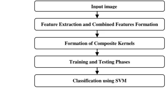
As a feature is the significant representative of an image, it can be used to distinguish one class from other. Feature extraction is the significant process while classifying the images. The extracted features exhibits characteristics of input pixel which the basic requirement of the classifier to make decisions about the class belonging of the pixels. The spatial features are extracted from Gray Level Co-occurrence Matrix (GLCM) and Gray Level Run Length Matrix (GLRM) and by Principal Component Analysis and Independent Component Analysis. After extracting such features they are to be combined to form the Combined Features. The Proposed work flow is shown in figure 1.
3.1.1. Extraction of Gray Level Co-occurrence Features
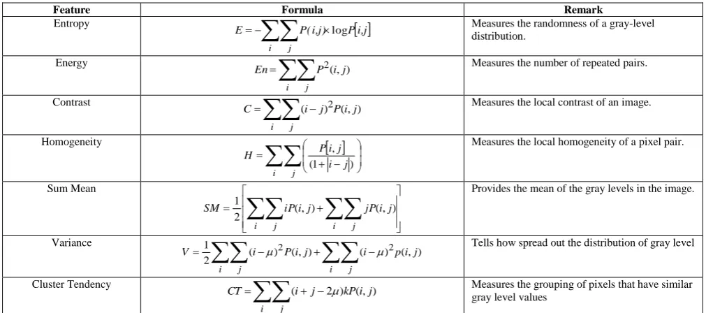
the formulas shown in Table 1. While calculating the features, „1‟ distance and „00‟ direction is considered for this experiment
Figure 1. Proposed Work Flow
From the GLCM P(i, j), many texture measures can be calculated. The features derived from run-length statistics are shown in table 1.
3.1.2. Feature Normalization
The scales of the eleven different features varied greatly, so they were normalized. The features need to be normalized so that no one feature dominates the others. A feature vector was calculated for each of the images. Form this set of data, a single combined mean feature vector (µ) and a single combined standard deviation vector (
x) are calculated using the combined data from all the classes in the training set. The normalization is done by using the equation (1).x i I
x X
, (1) 3.1.3. Extraction of Run Length Features
For a given image, an element P(i,j) in the run length matrix „P‟ is defined as the number of runs with gray level „i‟ and run length „j‟. The Run-Length Matrices are calculated in all the four directions (00, 450, 900, 1350). From each Run-Length Matrix, the features are extracted.From the run-length matrix P(i, j), numerical texture measures can be computed and are known as run Length Features. The features derived from run-length statistics are shown in table 2. Where P is the run-length matrix, P (i,j) is an element of the run-length matrix at the position (i,j) and „nr‟ is the number
of runs in the image. Most features are only functions of run length and not considering the information given by the gray level where as in Co-occurrence features the gray levels are significantly included. So, the Run Length features can able to provide extra spatial information about the classes.
3.1.4 Extraction of Principal Components
PCA is optimal in the mean square sense for data representation. So, the Hyper spectral data are reduced from several hundreds of data channel into few data channels. Hence the dimensionality can also be reduced without losing the required information.
The steps involved in Principal Component Extraction are as follows: 1. Get the image
2. Calculate mean and Co-variance matrix
3. Calculate Eigen vectors from the Co-variance matrix 4. Find Eigen values
5. Order the covariance matrix by Eigen value highest and lowest
6. Eigen vectors with highest Eigen value is the Principal Component, which contains significant information 7. Lowest Eigen value components can be discarded
The significant components known as Principal Components can be used as the features for classification as they depict more information about the image and are good representatives of image.
Input image
Feature Extraction and Combined Features Formation
Formation of Composite Kernels
Training and Testing Phases
3.1.5 Extraction of Independent Components
It is a statistical technique which reveals the hidden factors. As ICA separates the underlying information components of the image data, it can be used as a feature extraction technique. ICA generates the variables which are not only decorrelated, but also statistically independent from each other. PCA makes the data uncorrelated while ICA makes the data as independent as possible. This property is useful in discriminating the different classes in the image.
Table 1. Co-occurrence Features
ICA features can be used for classification, as they exhibits high order relationship among image pixels and ICA seeks to find the directions of projections of the data.
Table 2. Run Length Features
ICA features are higher order uncorrelated statistics. While PCA features are second order uncorrelated statistics. Second order statistics may inadequate to represent all the objects in the image. To exploit the information from the multivariate data such as hyper spectral data, higher order statistics are required. ICA features are capable of finding the underlying sources in such applications in which PCA features fail.To identify the independency between classes the linear transformation is required. If the pixels in the corresponding classes depicts zero Mutual Information,
Feature Formula Remark
Entropy
i,j P P( i,j) E i j log
Measures the randomness of a gray-leveldistribution. Energy ) , ( 2 j i P En i j
Measures the number of repeated pairs.
Contrast
) , ( ) (i j2Pi j C
i j
Measures the local contrast of an image.
Homogeneity
i j i j
j i P H ) 1 (
, Measures the local homogeneity of a pixel pair.
Sum Mean
i j i j
j i jP j i iP
SM (, ) (, ) 2
1
Provides the mean of the gray levels in the image.
Variance ) , ( ) ( ) , ( ) ( 2
1 2 2
j i p i j i P i V
i j i j
Tells how spread out the distribution of gray level
Cluster Tendency
i j j i kP j i
CT ( 2) (, ) Measures the grouping of pixels that have similar gray levelvalues
Feature Formula Remark
Short Run Emphasis (SRE)
M i N j r j j i P n SRE 1 1 2 ) , (1 Measures the distribution of short runs. The SRE is highly dependent on the occurrence of short runs and is expected large for fine textures
Long Run Emphasis (LRE)
M i N j r j j i P n LRE 1 1 2 ). , (1 Measures distribution of long runs and highly dependent on the occurrence of long runs and is expected large for coarse structural textures
Gray Level Non uniformity (GLN) 2
1 1
) , (
1
M i M J r j i P n GLN
Measures the similarity of gray level values throughout the image. The GLN is expected small if the gray level values are alike throughout the image
Run Length Non uniformity (RLN)
N j M i r j i P n RLN 1 2 1 ) , ( 1Measures the similarity of the length of runs throughout the image. The RLN is expected small if the run lengths are alike throughout the image
Run Percentage j j i P n RPC r * ) , (
the non-Gaussianity of the projection for the data . For the pixel vectors are denoted as X, the steps involved in Independent Component Extraction are as follows:
1. Choose an initial weight vector Choose an initial weight vector W
2. Let . Where the function is the derivative of a
non-quadratic nonlinearity. 3. Let
4. If not converged, go back to 2
5. Repeat the process until converges. The extracted components are Independent Components. 3.1.6 Formation of Combined Features
The extracted Co-occurrence, Run Length features, Principle Components and Independent Components are combined as shown in table 3 and are used for classification.
Table 3. List of Combined Features
3.2. Support Vector Classifier
Support Vector Machines use the statistical learning theory which maximizes the distance between training samples of two classes. This approach gives SVMs a high generalization capacity which requires only a few training samples without compromising accuracy requirement and outperforms other classifiers.
For a given labelled training set {( ( }, is the training sample and is the corresponding label. For each training sample , the function yields f( ) ≥ 0 for =+1, and f < 0 for =-1. In other words, training samples from the two different classes are separated by the hyper plane
f(x) = + b=0. (2)
Mathematically, this hyper plane can be found by minimizing the cost function as shown in equation (7).
J(w)= w = ∥w∥2
(3)
subject to the separability constraints
+ b ≥+1, for =+1 (4)
or
+ b ≤-1, for =-1;i=1,2,. . .,N (5)
This specific problem formulation may not be useful in practice because the training data may not be completely separable by a hyperplane. On adding the slack constraints in equation, it will be modified as
( + b) ≥ 1- , ≥0; i=1, 2. . . N. (6)
For practical hyperspectral data,the Cost function can be added with equation (2) J(w, ξ)= ∥w∥2
+ C (7)
where C is a user-specified, positive, regularization parameter and the variable ξ is a vector containing all the slack variables =1,2,. . .,N.Support vector Machines performs the robust non-linear classification with kernel trick. SVM finds the separating hyper plane in some feature space inducted by the kernel function while all the computations are done in the original space itself. For the given training set, the decision function is found by solving the convex optimization problem.
1. Combined Feature Label Formed by
2. Combined Feature-I CF-I Summation of the extracted Co-occurrence Features
3. Combined Feature-II CF-II Summation of the extracted Run Length Features
l i i i i l i j i j l j i i j i i y and C to subject x x K y y g 11 , 1
0 0 ) , ( 2 1 ) ( max
(8)
Where ‘
‟are the Lagrange co-efficient. „C‟ is a positive constant that is used to penalize the training errors and „K‟ is the kernel. Optimal solution is found, by looking to which side of the hyper plane it belongs by using the decision functionf
(
x
)
implemented by the classifier for ant test vector.
l i i iiyk x x b
x f 1 ) , ( sgn )
( (9)
Composite kernels are formed by the different combination set of GLCM and GRLM features using RBF kernel function. It fulfills the Mercer‟s Kernel condition. For an input space X, if there is a mapping φ:X → H that maps any x, z ξ X into a Hilbert space H, then a kernel:X × X → R, is constructed as K(x, z) =<φ(x), φ(z)>H, where
<・, ・>H is the scalar product operator in H. Such kernel functions K satisfy the Mercer condition: the kernel matrix
formed by restricting K to any finite subset of X is positive semi-definite, and hence K is usually termed as Mercer kernels.
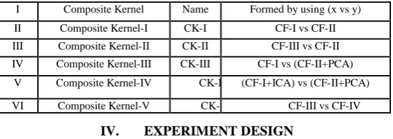
2 2 2 exp ) , ( z x z x K (10) 3.3 Formation of Composite Kernels
As the classifier parameters like kernels have their own impact on accuracy, the kernel formation and kernel selections are also equally important as feature extraction. The kernel is a function that maps the pairs of vectors to real numbers or positive definite. Kernel function can project the vectors from the high dimensional input space into the feature space. As feature space is comparatively low dimensional, the classification process is easy in this space. Choosing proper kernel amounts to choosing accurate feature space. It is the fundamental need to increase the accuracy. Available kernel is going to be modified to account for the cross relationship between the derived features. Weighted Summation Kernel algorithm is adopted to form the Composite Kernels of positive definite value. This Composite Kernels balance the Co-occurrence features, Run Length features, Principle Component Information, Independent Component Information which is the
fundamental need for multi-class classification problems. To solve high dimensional data classification problem, the following Composite Kernels are used as in equations (11) to (15). The formed composite kernels are shown in table 4.
(11)
(12)
(13)
(14)
(15) where is a positive definite parameter which is tuned during the training process. Tuning of gives a tradeoff between the derived features and which is useful to classify the given pixel.
: Co-occurrence Kernel Matrix
: Run Length Kernel Matrix
: Co-occurrence Kernel Matrix + Independent Component Kernel Matrix
: Composite Feature Vector-I
: Composite Feature Vector-II
: Composite Feature Vector-III
: Composite Feature Vector-I+ Extracted Principal Component Vector : Composite Feature Vector-II+ Extracted Independent Component Vector
Table 4. Formed Composite Kernels
IV. EXPERIMENT DESIGN
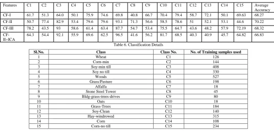
For evaluating the performance of the proposed method, a sample Hyper Spectral Image which is taken over northwest Indiana‟s Indian pine test site is selected. The site is sensed by AVIRIS. The data consists of 220 bands and each band consists of 145 x 145 pixels. The original data set contains 16 different land cover classes Co-occurrence and Run Length Features are calculated for the first fifty bands. Principle Components are calculated for the next fifty bands. Independent Components are calculated for the other fifty bands. First ten Principal Components are used since they contain 99.7% of the information. As it is not the case for Independent Components, all the Independent Components are used. Combined features are made as shown in Table 3. Composite Kernels are formed by using the derived Combined Features. The classification details with training information are shown in Table 6. The performance is validated in the testing phase and the accuracies are quantified and are shown in Tables 5 and 7.
V. RESULTS AND DISCUSSIONS
Pixels are randomly chosen from each class and their features are used for training. All other pixels are tested against the training samples.The classifier produces the output, whether the pixel under test belongs to the interested trained class or not. Thus the pixels of interested classes are identified among the whole data set. Similarly other classes are also trained. Randomly selected pixels are tested against the training samples. By this way, classes are separated hierarchically. After identifying the pixels of interested class it is labeled and indicated by white gray level. All other pixels are assigned black gray level. Then the pixels are displayed. The output is subtracted from the labeled ground truth and number of misclassified pixels is calculated. The accuracy of each class is calculated and is shown tables 6 and 7. By observing the accuracies, it is evident that the Composite Kernels yield the good accuracies for all the classes than the base kernels.The Co- occurrence and Run Length features are performing equally while they are separately used. The combination of Co-occurrence Features and Principal Components emit comparatively good accuracy than the traditional Co-occurrence feature set. Run Length features along with Independent components exhibit slight increment in the accuracy than the simple Run Length features. Except for few classes the combination of features shows increase in the accuracy.Corn-no till, Corn-Min-till, Soy-no till, Soy-min, Soy-Clean are the most similar classes and their texture variations are also similar. For these classes the conventional features exhibit lower accuracies.
But at least one of the proposed Composite Kernels give better result as they provide the cross-information such as Co-occurrence features, Run Length features, Principal Component information and Independent Component information.The spectral responses of the pixels belong to Soy-no till, Soy-min classes are similar. For these cases, the proposed kernels evidence slightly high accuracies than the Spatio-Spectral Composite Kernels available in the
I Composite Kernel Name Formed by using (x vs y)
II Composite Kernel-I CK-I CF-I vs CF-II
III Composite Kernel-II CK-II CF-III vs CF-II
IV Composite Kernel-III CK-III CF-I vs (CF-II+PCA)
V Composite Kernel-IV CK-IV (CF-I+ICA) vs (CF-II+PCA)
literature. Since in Spatio-Spectral Composite Kernels, any one of the spatial features are alone used. But in the proposed algorithm the combined features are used. So it provides the enhanced accuracy. In coarse texture like Alfafa, the gray level runs are longer. But fine texture like buildings takes the short runs. Likewise, the runs of gray levels are varying for each class. So, it is possible for classifying the classes by using Run Length features. For classes like Soybean-min, Alfalfa, the Run Length features have the potential for high accurate classification.
But Run Length features fail to distinguish the classes which contain more or less same textural properties. For identifying those classes, which are outliers while using the traditional Run Length features, Principal Components and Independent Components are used. For the class Soy-min, the Run Length features predominates the Co-occurrence features since Soy-min class has the good primitive information for classification which can easily be captured by the Run Length features. The availability of training samples is low for the classes like Alfalfa, Stone Steel Towers, Oats for which, the Principal Components, Independent Components with Co-occurrence features and Run length features respectively advocates good results. But it is not the case for Grass Pasture where both Canonical Analysis methods fail. This combination does not provide helping hand to the classes like Hay and Grass-Pasture mowed. Alfalfa and Grass-Pasture mowed which are assimilated by the neighboring classes. For the class, Woods the conventional methods and formed Composite Kernels are performing equally. But majority of the classes cast their vote to the Composite Kernels alone. Comparison of the measured accuracies are shown in figure 5.
Table 5.Classification Accuracy Details using the derived Features and RBF Kernel
Table 6. Classification Details
Features C1 C2 C3 C4 C5 C6 C7 C8 C9 C10 C11 C12 C13 C14 C15 Average
Accuracy CF-I 61.7 51.3 64.0 50.1 75.9 74.6 69.8 40.8 66.7 70.4 79.4 58.7 72.1 50.1 69.63 68.27
CF-II 50.7 77.4 82.9 53.4 79.6 79.6 93.1 71.3 56.6 58.5 78.6 51 52.1 53.1 44.6 70.22
CF-III 78.2 43.5 93 58.6 61.4 63.4 87.7 54.7 53.4 75.5 64.7 43.6 48.2 57.9 72.19 68.32
CF-II+ICA
64.3 54.4 92.1 55.9 69.6 62.5 96.5 41.6 56.2 81.7 68.5 40.3 40.9 45.7 64.82 66.83
Sl.No. Class Class No. No. of Training samples used
1 Wheat C1 126
2 Corn-min C2 144
3 Soy-min till C3 408
4 Soy no till C4 330
5 Woods C5 527
6 Grass/Pasture C6 198
7 Alfalfa C7 18
8 Stone Steel Tower C8 45
9 Bldg-grass-trees-drives C9 80
10 Oats C10 18
11 Grass-Trees C11 184
12 Soy-Clean C12 140
13 Hay-windrowed C13 315
14 Corn C14 108
Figure 5. Measured Accuracies using Combined Features and by Composite Kernels
Even though the Indiana Pines Data set has low spatial resolution and has mixed pixel effects, the proposed Composite Kernels yield better results than the base kernels. As these Composite Kernels are useful for class specific applications, one can choose this for their domain specific applications too.
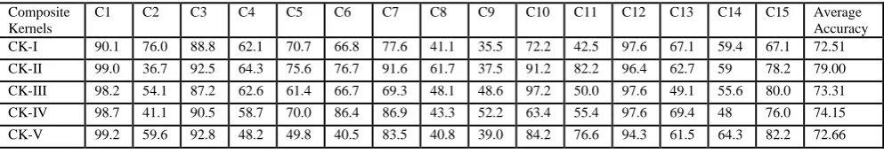
Table 7.Classification Accuracy Details for the Proposed Composite Kernels
VI. CONCLUSION
Even though the proposed Composite Kernels produces slight increment in the accuracy, this may be useful in cases where as the spectral features are not available. One can choose any one of the proposed kernels for class-Specific Applications. It is possible to develop a soft classification algorithm for this type of sensitive classifications. For this case of analysis, knowledge about „which‟ class a pixel belongs to is not sufficient. If, the information about, „how much‟ the pixel belongs to a particular class is known, it will be more useful for classification. As the Soft Classification extends its application to the sub-pixel levels, it can able to reduce the misclassifications.
ACKNOWLEDGEMENT
The authors are grateful to Prof. David. A. Landgrebe and Prof. Larry Biehl for providing the AVIRIS data set along with the ground truth and for providing the MultiSpec package.
REFERENCES
[1] David Landgrebe, “Some Fundamentals and Methods for Hyper Spectral Image Data Analysis”, SPIE Photonics, pp.1-10, Jan-1999. [2] G. F. Hughes, “On the mean accuracy of statistical pattern recognizers”, IEEE Transactions on Information Theory, IT-14(1) (1968).
[3] R. M. Haralick, K. Shanmugam, I. Dinstein, “Texture features for image classification.” IEEE Transactions on System Man Cybernetics, 8(6) (1973).
[4] Soe Win Myint “A Robust Texture Analysis and Classification Approach for Urban Land-Use and Land-Cover Feature Discrimination “, in the Proceedings of International Geocarto Conference at Hong Kong, 16(4), December 2001.
[5] Arivazhagan, S., Ganesan, L., “Texture Classification using Wavelet Transform”, Pattern Recognition Letters, 24 (2),2003.
[6] Arivazhagan, S, Ganesan, L., DeivaLakshmi, S, “Texture Classification using Wavelet Statistical Features”, Journal of the Institution of Engineers (India), 85 (1) (2003).
[7] Hiremath, P.S. and Shivashankar, S., “Wavelet Based Features for Texture Classification”, GVIP Journal, 6(3) (2006). [8] Galloway,”Texture information in Run Length Matrices”, IEEE Transactions on Image Processing, 7(11) (1975)
[9] Horng-Hai Loh, Jia Guu Leu,” The Analysis of natural Textures using Run Length Features”, IEEE Transactions on Industrial Electronics, 35(2) (1988). [10] Xiaoou Tang, ”Dominant Run- Length Method for Image Classification” Department of Applied OceanPhysics and Engineering, Woods Hole Oceanographic
Institution, Woods Hole, Report,WHOI-97-07,June 1997.
60 65 70 75 80
CF
-I
CF
-II
CF
-III
CF
-II
+IC
A
CK
-I
CK
-II
CK
-III
CK
-IV
CK
-V
Pe
rc
en
ta
g
e
A
cc
u
ra
cy
Features/ Kernels
MEASURED ACCURACY
Average Accuracy
Composite Kernels
C1 C2 C3 C4 C5 C6 C7 C8 C9 C10 C11 C12 C13 C14 C15 Average
Accuracy CK-I 90.1 76.0 88.8 62.1 70.7 66.8 77.6 41.1 35.5 72.2 42.5 97.6 67.1 59.4 67.1 72.51
CK-II 99.0 36.7 92.5 64.3 75.6 76.7 91.6 61.7 37.5 91.2 82.2 96.4 62.7 59 78.2 79.00 CK-III 98.2 54.1 87.2 62.6 61.4 66.7 69.3 48.1 48.6 97.2 50.0 97.6 49.1 55.6 80.0 73.31
CK-IV 98.7 41.1 90.5 58.7 70.0 86.4 86.9 43.3 52.2 63.4 55.4 97.6 69.4 48 76.0 74.15