Reliability analysis of building frames for seismic forces
T. Naqvi, T.K. Datta and G.V. Ramana
Indian Institute of Technology, Department of Civil Engineering, Hauz Khas, New Delhi – 110016, India.
ABSTRACT
A probabilistic risk analysis of steel building frames is presented using the hazard curve and the risk consistent response spectrum as inputs. The effect of soil amplification is duly considered for constructing the hazard curve and the response spectrum. The probability of failure of the frame is calculated by using the method of plastic analysis (mechanism method) and the first order second moment theory of reliability analysis. Plastic analysis is performed with equivalent (static) lateral load due to seismic effect, and the existing gravity load for probable mechanism of failure. Uncertainties considered in the study include those produced due to variations of the input motion, system parameters, modeling of the system and analysis procedure, energy absorption during the hysteretic loop and damage concentration effect. The method of analysis is illustrated by obtaining the annual frequency of failure of a twelve-storied steel building frame located at a hypothetical site, surrounded by three point sources of earthquake. The effect of important parameters on the probability of failure of the frame is also investigated by a parametric study.
INTRODUCTION
Probabilistic Risk Analysis procedure, commonly known as PRA procedure, has been widely used as a technique for determining the vulnerability of structures to seismic forces. For important structures, PRA procedure is adopted for determining their safety against seismic hazard. The probabilistic seismic risk analysis of structures is as such very complex, and involves a number of considerations such as seismic risk of the region, soil amplification characteristics of the site, description of the risk consistent seismic input, modeling and analysis of structures considering nonlinear effects, damage concentration etc. It is not possible to consider all factors in the seismic risk analysis of structures considering all factors mentioned above. Therefore, simplified PRA procedures have been applied to determine the probability of failure of different types of structures subjected to earthquake by several researchers (for example,[7], [9], [10]). However, very few of the studies are aimed at providing a practical PRA procedure that can be adopted by practicing engineer for structures like building frames, which can have many modes of failure. Further, not many studies are made to investigate the sensivity of the probability of failure of structures to the variation of important parameters related to the seismic risk assessment of structures. Here-in, a practical method for the probabilistic risk analysis of building frames subjected to seismic excitation is presented .The hazard curve and the risk consistent spectrum at the bed rock level are obtained by considering three earthquake sources around the site. The modifications of the hazard curve and the response spectrum due to the effect of soil amplification are incorporated by the frequency domain spectral analysis. The response of the frame is obtained by a static analysis for the equivalent lateral load obtained from the risk consistent response spectrum of earthquake, and the gravity loads. The annual frequency of failure of the building frames is determined by using the fragility curve and the hazard curve. For obtaining the fragility curve, different failure mechanisms, like sway, beam and combined mechanisms of failure are considered, and the probability of failure of the frame is determined by the first order second moment theory of reliability analysis. The uncertainties included in the study are those of modeling of the system, inelastic action, concentration of hinges, earthquake input, and material behavior. The sensivity of the probability of failure to the variation of some important parameters is conducted through a numerical study on a twelve-storied model of a shear building frame.
SEISMIC INPUT FOR RISK ANALYSIS
Risk consistent response spectrum and hazard curves are used as inputs for performing the risk analysis of structures. For constructing them, three earthquake point sources are assumed to be located around the site where the structure is located. The annual occurrence of earthquake is modeled as a Poisson process and the hazard curve is obtained, following the method proposed by [1] , as
P(A ≥ a) = 1 – exp{− ν (A ≥ a)} (1)
ν (A ≥ a) is given by the following expression
ν (A ≥ a) = P (A a|mi)Pk(mi) i
k k
k ≥
ν
∑
∑
(2)SMiRT 16, Washington DC, August 2001 Paper # 1719
in which P(A ≥ a) is the annual exceedence probability, Pk(mi) and νκ represent the probability density function of magnitude
of earthquake and the annual occurrence rate of earthquake respectively for the k-th source, Pk(A ≥ ami) is the conditional
probability of peak ground acceleration (PGA), A exceeding a, for a given mi. Risk consistent response spectrum is obtained
by assuming that the ordinate of the normalized response spectrum (normalized by its maximum acceleration value) SN(T) is
an empirically determined function of magnitude M and epicentral distance R having a log-normal distribution. Following form of the empirical function is used here [5]
*
N
S
= ln SN(T) = a(T)M – b(T)lnR + c(T) (3)in which a(T), b(T) and c(T) are constants for a particular value of the period (T). These constants depend upon the seismic characteristics of the region and are taken from the reference cited above.
The conditional mean value of the natural logarithm of response spectrum for the k-th source is obtained as
∑
< ≤=
i
2 1
i k i * N *
Nk(T) S (m ,T)P (m |a A a )
S (4)
Considering all seismic sources, the conditional mean value (for a1< A ≤ a2) of SN*(T) is represented by the following equation [5]
) a A a ( P
) a A a ( P ) T ( k S ) T ( S
2 1
k k k
2 1
k k k
* N *
N
≤ < ν
≤ < ν
=
∑
∑
(5)
The conditional mean square SN*2(T)can be obtained by replacing the mean value by the mean square value in Eq. (4). Then, the conditional standard deviation is given as
) T ( S )} T ( S { )} T ( S
{ *N = *N 2− N*2
σ (6)
The conditional probability of any value, A exceeding any particular level, say a1, for a given mi , as required in Eq. (2), is
obtained using the following attenuation law [3] for PGA(cm/sec2)
A = 5600
e
.8mi(R + 40)−2 ; σlnA = 0 .64, R ≥ 15km (7)
The plot of SN*(T)vs T provides the 50th percentile response spectrum. The 84th percentile response spectrum is obtained by plotting
[
SN*( )
T + σ{ }
S*N( )
T]
vs T.MODIFICATION OF RESPONSE SPECTRUM DUE TO SOIL CONDITIONS
The attenuation law used for obtaining the PGA at the site and the normalized response spectrum as obtained from Eq. (5) are valid for the bedrock level. The site is assumed to have a uniform layer of soil of 20m depth over the bedrock. In order to obtain the risk consistent response spectrum for the free field ground motion, the effect of soil amplification is considered by a spectral analysis in which the power spectral density function (PSDF) of the ground motion, Sb(ω) at the base rock level is
related to the PSDF of free field ground motion, Sg(ω) as
Sg(ω) = Sb(ω)|A(ω)|2 (8)
( )
(
) (
[
)
]
2s V / H s
V / H 2 cos
1 A
ξω + ω
=
ω (9)
in which H is the thickness of the soil layer; Vs is the shear wave velocity and ξ is the percentage of critical damping of the
soil.
The PSDF of ground acceleration is constructed from the response spectrum using the following expression [2]
Sb(ω) =
2 f j
f 2
]
p
/
)
,
(
D
[
]
/
4
/
2
[
ξω
π
+
πτ
ω
ξ
0ω
+
ω
ω
θ θ+ θ
(10)
where ω is frequency in radians per second ; θ=3.0; ωf =0.705 ;τ is the duration of the earthquake;
p
f0is the peak factor forwhite noise and Dj(ω,ξ) is the ordinate of the risk consistent response spectrum. The mean peak value of the free field acceleration i.e. PGA at the ground surface is obtained from the PSDF as
(
PGA)
f =λ0xPf (11)Where λ0 is the area under the PSDF curve of the absolute acceleration of the free field ground. Pf is the peak factor, which
is obtained from the three moments of the PSDF of the absolute acceleration of the free field ground motion[11]
(
)
[
]
{
}
[
ln2]
1/2e exp 1 2 ln 2 f
P = Γ − − − δ π Γ (12)
in which Γ is a function of time duration of earthquake and central frequency; δe is a measure of the spread in the frequency
content of the response power spectral density function about its central frequency.
Since an equivalent lateral load analysis is performed to obtain the seismic response of the building frame, the response spectrum for the free field ground motion is obtained from the PSDF of the free field ground motion using the inverse relationship given by Eq. (9).
FRAGILITY ANALYSIS OF THE BUILDING FRAME
An equivalent lateral load analysis is performed to obtain the response of the frame using modal response spectrum analysis. For this purpose, equivalent shear force at each story level is obtained by combining the shear forces in each mode by SRSS rule. The equivalent lateral load is constructed back from the story shears. For an assumed value of PGA, the response of the frame is obtained from the equivalent lateral load analysis using 50th percentile response spectrum. It is multiplied by four factors F1, F2, F3 and F4 in order to take into consideration the uncertainties produced due to variations of
the input motion, system parameter, modeling of the system and analysis procedure. F1, F2, F3 and F4 are considered as
random variables with prescribed mean values and standard deviations. Further, these random variables are assumed to be log normally distributed. Capacity of the frame elements to resist the action of the load is multiplied by two random factors F5
and F6 in order to consider the uncertainties introduced due to energy absorption during the hysteretic loop and damage
concentration respectively. Both F5 and F6 are assumed to be log normally distributed random variables with specified means
and standard deviations.
For obtaining the fragility curve, a failure mode for the frame is assumed, and the probability of failure is determined for that particular mode. The probabilities of failure are computed for all possible failure modes. For this purpose, the plastic analysis of the frame for different mechanisms of failure is carried out. Generally, those collapse mechanisms are considered which have relatively less values of collapse load factor. The probability of failure is computed by finding the bending moment (M) at the cross section where the last hinge is formed and by determining the moment capacity (Mp) for that section. The median values of resistance (R) and capacity (C) used for finding the probability of failure, pf = P(R< C) are
obtained as
R
~
= M F′1 F′2 F′3 F′4 andC
~
= Mp F′5F′6 (13)
σlnR = √(β12+ β22 +β32 +β42)
and σlnC = √(β52+ β62 + β2),
in which βi , i =1 to 6 are the logarithmic standard deviations of factors Fi , i = 1 to 6 and β is the logarithmic standard
deviation of Mp. Note that for log normally distributed random variables, σlnX 2 = ln (δX2 +1) and for δX ≤ 0.25 σlnX = δXin
which δX is the coefficient of variation of the random variable x. First order second moment (FOSM) technique is used to
calculate the probability of failure by assuming both resistance (R) and capacity (C) to be log normally distributed [6] i.e. )
0 ) X ( g ( p
Pf = <
) C R (
P <
=
) 1 C / R (
P <
=
let Z=R/C (14)
Since R and S are independent and log-normally distributed, then Z also is log normally distributed with mean µlnz and
standard deviation σlnz given by
( )
= = µC~ R~ ln Z ~ ln z
ln (15)
2 C ln 2
R ln z
ln = σ + σ
σ (16)
The probability of failure pf is expressed as
(
lnZ 0)
P
Pf = <
σ
µ − Φ =
z ln
z ln 0
) (−β Φ
= (17)
where Φ( ) is standard normal distribution function and β is the reciprocal of the coefficient of variation of the logarithmic variate.
The annual frequency of failure is obtained by combining the fragility curve and the hazard curve. It is a plot between the annual frequency of exceedence versus probability of failure.
DETERMINATION OF MEDIAN AND COEFFICIENT OF VARIATION OF THE FACTORS (Fi)
Factor F1 caters to the uncertainty of the input motion. It is assumed to be log normally distributed random variable with
median value as unity and the logarithmic standard deviation β1 as the ratio of two response values corresponding to input
motions of the median and 84% non-exceedance spectra ie, β1 = ln ( r 84 / r 50 ). Factor F2 caters to the uncertainty of the
material property. It is assumed to be log normally distributed random variable with median value as unity. The logarithmic standard deviation β2 is evaluated in the same manner as for the case of factor F1. Factor F3 caters to the uncertainty of the
structural modeling. F3 has a median value of unity and coefficient of variation ranging between 0.15 and 0.2 as obtained
from several studies on the effect of structural modeling on response [10]. F4 is the factor accounting for the uncertainty
resulting from the simplification of the method of analysis like, nonlinear analysis being replaced by equivalent linear analysis; dynamic analysis being replaced by equivalent static analysis; simulation analysis being replaced by the ratio between percentile responses etc. The median value of F4 is assumed as unity and the coefficient of variation is assumed to
range between 0.1 and 0.15 [10]. Factor F5 caters to the energy absorption during nonlinear excursion of a SDOF system. The
median value is generally taken to be proportional to Newmark’s formula √(2µ -1) with a reduction factor of 0.6, where µ is the ductility factor. The coefficient of variation is taken about 0.2. Factor F6 caters to the damage concentration effect of
MDOF systems. The median value of F6 is evaluated as (QL/QNL)/0.6 √(2µ -1); in which QL and QNL are linear and nonlinear
stresses respectively. Extensive numerical studies on complex structures showed that the median value of F6 typically ranges
NUMERICAL EXAMPLE
As a numerical example, a twelve-storied steel frame is considered as shown in Figure 1. The properties of the members are shown in Table 1. It is assumed to be on a site which is surrounded by three point sources which are at distances of 153.05 m; 253.14 m and 87.5 m respectively from the site. The annual occurrence rates of earthquake for the three sources are 4.1, 2.83 and 0.8 respectively. The probability density function of the magnitude of earthquake is taken to be of the form e–m/b,with the value of b for each source as 0.7. The frame is designed according to Indian code of practice for a PGA value of 0.05g. The properties of the frame and the gravity loads acting on different beams are given in Table1. For the combination of the equivalent lateral loads and the gravity loads on the frame, different collapse mechanisms are possible like, sway, beam and combined mechanisms. Out of the possible mechanisms three mechanisms are considered in the study, which have relatively less values of collapse load factor. The mechanisms are shown in Figure 2. Probabilities of failure are determined for these collapse mechanisms.
Shear wave velocity (Vs) of the soil layer over the bedrock is assumed to be 200 m/sec. The seismic input to the frame is
taken as the normalized free field response spectrum for Vs = 200 m/sec as shown in Figure 3, for the PGA interval of 0.21g
to 0.25g. Effect of the soil characteristics on the seismic inputs and the probabilities of failure of the frame are studied by varying the value of Vs in the parametric study.
Table 1: Properties of the frame
Member 1 to 7 and 25 to 31 ISHB250
Member 8 to 12 and 32 to 36 ISHB225
Member 13 to 16 ISHB300
Member 17 to 19 ISHB250
Member 20 to 24 ISHB225
Member 37 to 84 ISWB350
Equal bay width = 6m
Storey height = 3m
Moment of resistance of outer columns = 200KNm Moment of resistance of outer columns = 275 KNm Moment of resistance of beams = 120KNm Point load at the centre of each beam = 11.0KN Cov for point load and moment of resistance = 0.1
Figure 1: Building frame
Figure 2: Mechanisms of failure
A
•
•
B
•C
D
(a) Mech - a
• • • • • • • • • • • • • • • • • • •
• • • • • • • • • • • • • • • • • • • • • • • • •
• • • • • •
(b) Mech - b
•• ••
• • • • • • • •
• • • • • • • • •• •• •• •• •• •• •• •• •• •• •• •• •• ••
(c) Mech - c
Effect of the Formation of the Last Hinge
In the sequential analysis, the probability of failure is calculated for each successive formation of hinges and the final probability of failure is determined from that corresponding to the last hinge formed in the structure. The above procedure is computationally intensive and therefore, simplified analysis is performed by assuming a collapse mechanism and the probability of failure is computed by assuming different hinges to form as the last hinge in the structure. For the present example problem, it is observed that the probability of failure remains nearly the same if the last hinge is formed at any of the identified positions (A,B,C or D) as shown in fig 1. A similar trend is observed for the other two mechanisms. Thus, by a limited number of trials, the probability of failure corresponding to a particular mechanism can be obtained. This procedure of obtaining the probability of failure is much less time consuming and simpler than the sequential analysis especially for large framed structures. For further parametric study the probabilities of failure are calculated by assuming the last hinge to be forming at the base of any column.
(a)Normalised Response Spectrum 0
5 10 15 20
0 1 2 Period(sec)3 4 5
Norm. Acc.
freefield bedrock
(b) Hazard curve
0 0.5 1 1.5
0.01 0.21 0.41 PGA(g)
Annual Exceed.
Prob.
bedrock freefield
Figure 3: Risk consistent seismic input
Effect of the Assumed Mode of Collapse
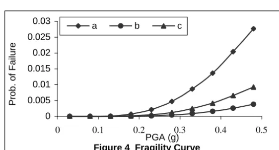
The fragility curves for the three assumed mechanisms of failure are shown in fig 4. It is seen that the pure sway mechanism of failure-a (fig 2) gives the highest probability of failure. The combined mechanisms-c (fig 2) of failure gives the lowest value of probability of failure. Thus for obtaining the fragility curve a pure sway mechanism is considered in the analysis. For further parametric study mechanism-a is used.
Figure 4 Fragility Curve
0 0.005 0.01 0.015 0.02 0.025 0.03
0 0.1 0.2 0.3 0.4 0.5
PGA (g)
Prob. of Failure
a b c
Effect of the Standard Deviation of Factors F(i) (i=1 to 6)
Fragility curves as shown in figure 4, are obtained with the values of β1 to β6 as given in the first row of Table 2.In order
to investigate the effect of the variation of logarithmic standard deviations of the factors Fi (i=1 to 6) on the Pf, they are
changed one at a time. Note that the logarithmic standard deviation of the factor F1 is not changed since it remains fixed once
the risk consistent response spectrum is generated. It is seen from the table that the individual change in the standard deviation of the factors except β2, does not have significant influence on the probability of failure. The change in β2 (i.e.,
Table 2: Sensivity study of different parameter (PGA=.23g)
β1 β2 β3 β4 β5 β6 Probability of failure
.49 .46 .3 .15 .14 .25 0.00216
.49 .3 .3 .15 .14 .25 0.00077
.49 .46 .15 .15 .14 .25 0.001283
.49 .46 .3 .3 .14 .25 0.003309
.49 .46 .3 .15 .2 .25 0.002479
.49 .46 .3 .15 .14 .1 0.001455
.49 .46 .3 .3 .2 .25 0.003708
.49 .3 .15 .15 .14 .1 0.000156
Effect of ductility
For the computation of probability of failure, the median values of factors F1 to F4 are taken as unity, whereas the median
value of F5 is calculated using Newmark’s formula, which depends on the ductility factor µ. Thus, the ductility factor is
expected to have an effect on the probability of failure. It is seen that as ductility increases the probability of failure significantly decreases. For example, for µ = 2, Pf = 0.013262; whereas for µ = 5, Pf = 0.001839 ( for a PGA level of 0.23g).
Effect of Soil Property
The hazard curves and the normalized spectrums for the bedrock level and the ground surface are shown in figure 3. It is seen that the peak of the response spectrum for the bed rock is amplified nearly seven times when the bedrock motion is filtered through a 20 km soil layer with Vs = 200m/sec. Similarly, the hazard curve shows a significant increase in the value of PGA being exceeded, when the bed rock motion is filtered through the same layer of soil. Thus, the probability of failure of the frame may be significantly influenced by the effect of soil properties since risk consistent seismic inputs are drastically changed by the effect of soil layer above the bedrock. In order to investigate the effect of soil property on the probability of failure, the risk consistent normalized seismic response spectrums are obtained for three-shear wave velocities (Vs) namely
80, 150 and 200 m/sec. The probabilities of failure are obtained as Pf = 2.09E-06 for Vs = 80 m/sec; Pf = 6.03E-09 for Vs =
150 m/sec; Pf = 2.61E-09 for Vs = 200 m/sec for a PGA value of .03g. It is seen that the probability of failure can be
substantially increased for the soft soil condition even for a small value of PGA. Thus, the effect of soil conditions should be duly incorporated in calculating probabilities of failure by way of modifying the seismic inputs.
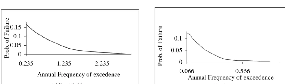
In order to investigate the effect of the soil layer on the annual frequencies of failure, they are obtained at the bedrock level and at the ground surface for a shear wave velocity equal to 200 m/sec. It is seen from figure 5 that annual frequencies of failure are substantially increased when the effect of soil layer above the bedrock is considered in the analysis. Note that the effect of the soil layer on the annual frequencies of failure is the result of two effects; one is that of hazard curve and the other is that of the risk consistent response spectrum.
(a) Free Feild
0 0.05 0.1 0.15
0.235 1.235 2.235
Annual Frequency of excedence
Prob. of Failure
(b) At Base 0
0.05 0.1
0.066 0.566
Annual Frequency of exceedence
Prob. of Failure
CONCLUSIONS
A methodology for obtaining the fragility curve and the consequent annual frequency of failure (and hence, the reliability against failure) is presented for building frames. For this purpose, risk consistent seismic inputs are considered which duly take into account the soil amplification effect. The uncertainties considered for the reliability analysis include those produced due to variations of the input motion, system parameters, modeling of the system and analysis procedure, energy absorption during the hysteretic loop and damage concentration effects. First order second moment theory of reliability analysis is used for calculating the probability of failure of the building frame. A twelve-storied building frame located at a site, which is surrounded by three point sources of earthquake, is taken as an illustrative example. The results of the numerical study show that:
1) Determination of the probability of failure of the building frame using the mechanism method of plastic analysis is computationally simpler and much less time consuming.
2) Position of the last hinge formed in a mechanism of failure does not have much effect on the probability of failure of the frame.
3) A combined sway mechanism of failure in the frame gives the highest estimate of the probability of failure.
4) Variation of the standard deviations of the uncertainty factors except β2, within possible range of values, does not have
large effect on the probability of failure; variation of β2 ie, variation of system property significantly influences the
probability of failure.
5) Nature of soil, indicated by its shear wave velocity, has a pronounced effect on risk consistent spectrum inputs and the annual frequency of failure of the frame.
6) Effect of ductility on the probability of failure of the frame could be significant and therefore, it should be carefully estimated.
REFERENCES
1. Der Kiureghian, A. & Ang, A.H.S..” A fault rupture model for seismic risk analysis”, Bull. of Seism. Soc. Am., 67(4),1977, pp.1173 - 1194.
2. Der Kiureghian, A. & Neuenhofer,A.,” Response spectrum method for multisupport seismic excitations”, Earthq. Engg. and Structural Dynamics, l 21, 1992, pp. 713-740.
3. Gupta, I.D., Rambabu,V&Gowda, B.M.R. 1997. An integrated PGA attenuation relationship, Bull. Ind. Soc. Earthq. Tech., 34: 137 - 158.
4. Kramer, S.L, Geotechnical Earthq. Engg. Prentice Hall, New Jersey , p p54 – 280, 1996.
5. Kiyoshi, I, Toshihiko, O. & Makato Suzuki. 1989. Earthquake ground motions consistent with probabilistic seismic hazard analysis,. Proc ICOSSAR 89, 5th Int Conf Struct Saf Reliab. ,pp.605-609, Publ by ASCE, New York, NY, USA. 6. Ranganathan, R. 1990. Reliability analysis and design of structs. New Delhi. McGraw-Hill.
7. Ravindra, M.K. 1989. Recent seismic risk studies of nuclear power plants. An overview , Proc ICOSSAR 89 ,5th Int Conf Struct Saf Reliab. ,pp.2211-2218, Publ by ASCE, New York, NY, USA.
8. Ravindra, M.K. 1990. System reliability considerations in probabilistic risk assessment of nuclear power plants, Structural Safety, 7,pp. 269-280.
9. Shinozuka, M., Mizutani, M., Takeda, M. and Kai, Y. 1989. A Seismic PRA procedure in Japan and its application to a building performance safety estimation. Part 3.Estimation of bldg. and equipment performance and safety. Proc ICOSSAR 89 5th Int Conf Struct Saf Reliab. , pp. 637-644, Publ by ASCE, New York, NY, USA.
10. Takeda, M., Kai, Y. and M. Matsubara. A Seismic PRA procedure in Japan and its application to a building performance safety estimation. Part 2.. Fragility analysis. Proc ICOSSAR 89 ,5th Int Conf Struct Saf Reliab. , pp. 629-636, Publ by ASCE, New York, NY, USA, 1989.