Real-time Contaminant Source Characterization in Water Distribution Systems

(1)

ABSTRACT

LIU, LI. Real-time Contaminant Source Characterization in Water Distribution Systems. (Under the direction of S. Ranji Ranjithan and G. Mahinthakumar.)

(2)

(3)

Real-time Contaminant Source Characterization in Water Distribution Systems

by Li Liu

A dissertation submitted to the Graduate Faculty of North Carolina State University

in partial fulfillment of the requirements for the Degree of

Doctor of Philosophy

Civil Engineering

Raleigh, North Carolina 2009

APPROVED BY:

_______________________________ ______________________________

Dr. E. Downey Brill, Jr. Dr. Emily M. Zechman

_______________________________ ______________________________

Dr. Sankar Arumugam Dr. G. Mahinthakumar

Co-Chair of Advisory Committee _______________________________

(4)

BIOGRAPHY

Li Liu was born and grew up in Shouxian, a small city in China that boasts of a history of thousands of years. She is the youngest daughter of Zhitian Liu and Wenlan Wang, and has three older sisters, Chuanjun, Chuanxia and Chuanling. Li entered Hefei University of Technology in China for her undergraduate studies after graduating from high school. Upon graduation with a Bachelors degree in Civil Engineering, she was engaged as a lecturer by the Department of Civil Engineering at Hefei University of Technology. In 2001, she elected to remain at Hefei University of Technology for her Masters degree, specializing in Systems Engineering of Water Resources under the direction of Dr. Juliang Jin. In January 2005, Li enrolled in the doctoral program at North Carolina State University in Raleigh, North Carolina, where her research focused mainly on contaminant source characterization in water distribution systems.

(5)

ACKNOWLEDGMENTS

I would like to express my sincerest appreciation to my advisor, Dr. Ranji Ranjithan, for his continuous support, intelligent guidance, patience and encouragement during the past four years. This research could not been completed without his assistance and efforts. I am also indebted to the professors in my committee, Drs. Downey Brill, Sankar Arumugam, and G. Kumar Mahinthakumar for their invaluable suggestions and time.

I would like to thank my graduate and research peers, Emily Zechman, Sarat Sreepathi and Jitendra Kumar for their assistance and helpful discussions in conducting research. Thanks also to my officemates, Yong Jung, Xin Jin, Matthew Clayton, Eiman Abbas, Michael Tryby, Ozge Kaplan, and Pamela Schooler for their friendship and encouragement.

(6)

LIST OF TABLES

Table 2.1 Parameters Settings for MPB... 17

Table 2.2 Comparison of Average and Standard Error of Generation Error for ADOPT and Multi-objective Optimization-based Methods by Bui et al. (2005) ... 17

Table 2.3 Sensitivity of Parameter Settings of ADOPT ... 18

Table 2.4 Description of Groundwater Simulation Parameters ... 24

Table 3.1 Allowable Range of Source Parameters for the Case Studies ... 42

Table 3.2 True Source Description for Four Contamination Event Scenarios ... 54

Table 4.1 Contaminant Source Parameters and Ranges for Generating Training Data Set ... 73

Table 4.2 Summary of Results under Various Uncertain Conditions... 75

Table 4.3 Statistical Summary of the LRM Results that Correspond to the Injection Node .. 79

Table 5.1 Allowable Ranges of Contaminant Source Parameters ... 96

Table 5.2 True Source Description for Five Contamination Event Scenarios... 97

Table 5.3 Number of Potential Nodes Obtained from the LRMs for Five Hypothetical Contamination Events... 98

Table 5.4 Summary of the LRM-LS Results for Five Hypothetical Contamination Events .. 99

Table 5.5 Summary of Results for Scenario 1 under Different Sensor Conditions... 103

Table 6.1. Allowable Ranges of Source Parameters... 125

Table 6.2 Parameter Settings of the (µ+λ) ES-based ADOPT... 125

(9)

LIST OF FIGURES

Figure 2.1 Comparison of average generation error for ... 20

ADOPT with different parameter settings ... 20

Figure 2.2 Variation of diversity with generation for ADOPT with different parameter settings ... 21

Figure 2.3 Comparison of ADOPT results at time steps 6, 8, and 10 for Scenario 1 and Scenario 2... 25

Figure 2.4 Results of ADOPT at time step 20 for Scenario 1... 26

Figure 2.5. Average number of the remaining subpopulations through time. ... 27

Figure 3.1 Layout of the small network... 43

Figure 3.2 Results for the base scenario using ES-based ADOPT ... 45

Figure 3.3 Results from different mutation strategies based on the base scenario ... 49

Figure 3.4 Effect of initial number of subpopulations on the ADOPT solutions ... 50

Figure 3.5 Effect of the number of generations on the ADOPT solutions. ... 52

Figure 3.6 Effect of the quantity and quality of monitoring data on the number of alternative solutions. ... 53

Figure 3.7 Four hypothetical contamination scenarios along with the base scenario:... 54

Figure 3.9 Micropolis water distribution network schematic ... 56

Figure 3.10 Identified solutions at 6:50 p.m. for the hypothetical contamination event in the micropolis network. ... 58

Figure 3.11 Identified solutions at 9:00 p.m. for the hypothetical contamination event in the micropolis network. ... 59

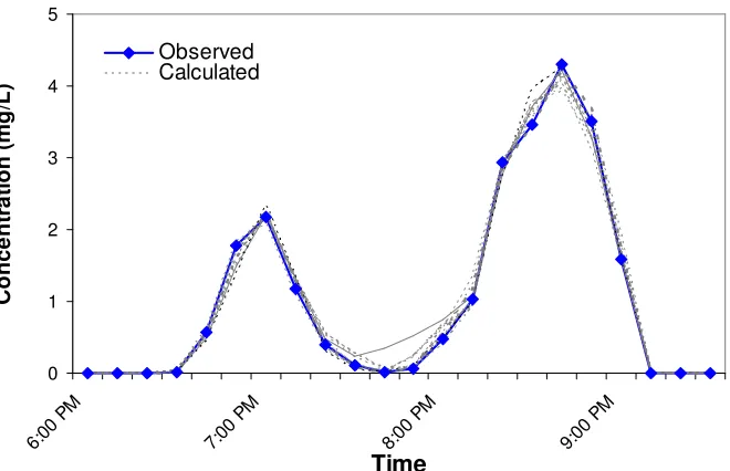
Figure 3.12 Comparison of concentration profiles between the observed and calculated profiles at S3 for the hypothetical event in the Micropolis network... 59

Figure 3.13 Comparison between the number of subpopulations and alternatives for a hypothetical event in the micropolis network ... 60

Figure 4.1 Water distribution network schematic (small network example)... 72

Figure 4.2 Comparison of performance of LRMs between Scenario 1 and Scenario 2: ... 74

Figure 4.3 Comparison of results between perfect and binary sensor conditions ... 77

Figure 4.4 Layout of micropolis water distribution network ... 80

Figure 4.5 Comparison of results between two model-building strategies (micropolis network). ... 82

Figure 4.6 Locations of possible sources at 12:30 p.m... 83

Figure 4.7 Locations of the top 50 solutions at 1:40 p.m. ... 83

Figure 5.1 Flowchart of LRM-LS model for contaminant source determination in a WDS. . 94

Figure 5.2 Layout of small example network ... 96

Figure 5.3 Illustration of injection locations for five hypothetical events ... 97

Figure 5.4 Comparisons of results for Scenario 1 under different sensor conditions... 102

Figure 5.5 Summary of results for 50 random contamination events... 104

(10)

Figure 5.7 Location of possible source locations at 12:30 p.m. ... 106

Figure 5.8 Location of alternative solutions at 1:40 p.m.: ... 107

Figure 6.1 LRM-ADOPT-LS optimization framework ... 122

Figure 6.2 Layout of the example networks ... 124

Figure 6.3 Comparisons of the results from different approaches... 127

Figure 6.4 Comparison of the results between LS selection strategies... 130

(11)

CHAPTER 1: Introduction

Municipal drinking water supply systems aim to provide safe drinking water to customers throughout an entire service area. These systems begin at water sources and convey drinking water to designated points after the water is treated through widely distributed municipal water networks that involve pipes, storage tanks, and pumps. Because the water network is wide and contains numerous possible access points, the system is vulnerable to possible threat, including physical attack, cyber-disruption, and biochemical contamination (Clark and Deininger, 2000). Biochemical contamination, either accidental or intentional, has become a major concern recently due to its inherent complications and the potential hazard to human health.

(12)

The accuracy of the characterization largely depends on the number and quality of the sensor observations. Ideally, the sensors installed in the network would provide perfect and contaminant-specific observations at each node in the water network. In reality, however, the data may be imperfect or may merely indicate the presence of contamination. The cost of sensor installation and monitoring discourages an adequate number of observations to be made, which further complicates the characterization.

Contaminant source characterization can be viewed as an inverse problem, which is typically ill-posed as opposed to a forward problem in which model parameters are known. For example, a contaminant with diverse strengths injected at different times and locations may yield similar explanations among the sensor observations. That is, current observations are unable to distinguish the true injection node from other potential nodes due to insufficient data. This non-uniqueness of solutions may result from limited data, model error, or measurement error, all of which contribute to the complexity of such a problem.

(13)

One way to address this problem is to formulate it as an optimization problem by making use of currently available observation data to inversely seek the best source characteristics. This formulation could yield a good explanation of the water quality samples that are obtained. Recently, various efforts have been made to develop approaches to address this problem. The optimization methods that have been applied include direct and simulation-optimization approaches. In van Bloemen Wannders et al. (2003), a standard successive quadratic programming tool is applied to solve a small-scale problem. Laird et al. (2005) present an origin tracking algorithm to address the inverse problem of contamination source identification based on a nonlinear programming framework. Taking advantage of a simulation-optimization approach, whereby a search procedure is coupled with a simulation model, Guan (2006) demonstrates its applicability to nonlinear contaminant source and release-history identification.

The limitations of the aforementioned work often include the inability to address non-uniqueness, deterministic characterization, small network size, high computational costs, etc. In the event of contamination, a well-developed algorithm must be able to: 1) dynamically update the determination of source characterization as the number of observations changes over time; 2) adaptively assess the degree of non-uniqueness and also identify non-unique solutions if available; and 3) quickly provide real-time solutions.

(14)

problems by coupling the simulation models. Evolutionary algorithms (EAs) (Holland, 1975), as one class of heuristic methods, present a global search (GS) mechanism and are of great benefit for solving large nonlinear optimization problems. EAs are also flexible enough to be extended to dynamic and noisy conditions. They have been used in several water distribution network design problems (e.g., Dandy et al., 1996; Savic and Walters, 1997). Although EAs have been used effectively to solve inverse problems, such as water distribution network calibration (e.g., Vitkosvsky et al., 2000; Lingireddy and Ormsbee, 2002) and groundwater source contamination identification problems (e.g., Mahinthakumar and Sayeed, 2005; Mahar and Datta, 1997), little is known about their applicability to source characterization in a water distribution systems (WDS) under dynamic and noisy conditions.

The primary objective of this study is to design a contaminant source characterization procedure for a WDS by integrating simulation models with a heuristic search-based optimization framework, given observation data that stream in over time, and to adapt this algorithm or couple it with some other method(s) for realistic source identification in the WDS. Overall, this dissertation has five main objectives:

1. Develop a new methodology, the EA-based Adaptive Dynamic OPtimization Technique (ADOPT), that can solve an optimization problem in dynamic environments.

(15)

3. Develop a fast estimation methodology to determine the likelihood that any given node is a potential source by processing the observation data obtained from monitoring stations in the WDS over time.

4. Investigate the applicability of coupling the proposed prescreening technique with heuristic search methods, such as ADOPT, local search methods or a combination of both, to improve the efficiency of the solutions.

5. Examine the effects of uncertainties on the resulting solutions of the proposed methods.

(16)

(17)

CHAPTER 2: An Adaptive Optimization Technique for

Dynamic Environments

Abstract. The use of evolutionary algorithms (EAs) is beneficial for addressing

optimization problems in dynamic environments. The objective function for such problems changes continually; thus, the optimal solutions likewise change. Such dynamic changes pose challenges to EAs due to the poor adaptability of EAs once they have converged. However, appropriate preservation of a sufficient level of individual diversity may help to increase the adaptive search capability of EAs. This chapter proposes an EA-based Adaptive Dynamic OPtimization Technique (ADOPT) for solving time-dependent optimization problems. The purpose of this approach is to identify the current optimal solution as well as a set of alternatives that is not only widespread in the decision space, but also performs well with respect to the objective function. The resultant solutions may then serve as a basis solution for the subsequent search while change is occurring. Thus, such an algorithm avoids the clustering of individuals in the same region as well as adapts to changing environments by exploiting diverse promising regions in the solution space. Application of the algorithm to a test problem and a groundwater contaminant source identification problem demonstrates the effectiveness of ADOPT to adaptively identify solutions in dynamic environments.

2.1. Introduction

(18)

interest involve time-dependent objective functions that gradually change with time. Examples of time-dependent dynamic optimization problems include dynamic vehicle routing, scheduling, and threat management problems. The commonality among these problems is that the environment, such as dynamic information and time-varying restrictions, is continually changing while decisions are being made. With the intention of effectively discovering optimal solutions in real time, an adaptive approach is required that not only determines the current optimum but also quickly adjusts the solutions to a new environment when change occurs.

A number of researchers have demonstrated that EAs, as a class of heuristic search methods, offer the potential to handle such optimization problems due to their population-based search properties (Holland, 1975). In the context of complex real-world optimization problems, the use of EAs is particularly beneficial because they can integrate complicated simulation models to evaluate objective functions effectively. However, as EA populations converge to the best solution for the current setting of the problem, they have difficulty adapting to the changing environment, limiting the application of traditional EAs to solve dynamic optimization problems. Nevertheless, various methods that extend the use of EAs for addressing such dynamic optimization problems have been developed in recent decades, including memory-based and diversity-based techniques.

(19)

later when a new environment emerges. The memory-based scheme has proved highly useful for the resolution of cyclical dynamic environment problems.

Another approach to solve dynamic optimization problems is to sustain adequate diversity while the environment changes. Several diversity-based approaches have been developed, such as maintaining diversity via random immigrants (Grefenstette, 1992), modifying selection processes (Ghosh et al., 1998; Goldberg and Richardson, 1987), multi-objective optimization (Bui et al., 2005), and multi-population techniques, such as self-organizing scouts (Branke, 2002), shifting balance genetic algorithms (GAs) (Oppacher and Wineberg, 1999), and multinational GAs (Ursem, 2000).

Hybrid approaches are a combination of different concepts, such as memory and diversity (Branke, 2002). Conceptually, this kind of approach incorporates the advantages of both memory and diversity schemes. An example of such a hybrid approach is a memory-based immigrant scheme within a GA, developed by Yang (2005), where the best solution is stored to generate random immigrants that potentially introduce the diversity of the search process in dynamic environments.

(20)

emerges. To allow a reasonable evaluation of the proposed approach, the previously developed multi-objective optimization-based method (Bui et al., 2005) is used as a base, and the results are compared with those of ADOPT via the Moving Peaks Benchmark (MPB) problem using the same parameter settings. In addition to illustrating the ability to adaptively maintain diversity, ADOPT’s ability to adapt to a changing environment is demonstrated through different algorithmic settings and problem scenarios. In this chapter, the framework is applied to a groundwater contaminant source characterization problem where the monitoring observations are dynamically updated. This adaptive capability results in an effective assessment and resolution of the degree of non-uniqueness of the solutions. The methodology is sufficiently general to be applicable to other time-dependent optimization problems in which the environment changes gradually between consecutive time steps.

2.2 Solution Approach

2.2.1 Evolution Strategy (ES) for Dynamic Optimization Problems

(21)

mutation step lengths (Yang, 2007). Once mutated, the step length is used to create a random vector to mutate the decision variables accordingly. Thus, the mutation strengths progress along with the individuals instead of through predetermined values. The ES has been demonstrated to possess a self-learning property, even in the dynamic context of an optimization problem (Hoffmeister and Back, 1992).

2.2.2 Adaptive Dynamic Optimization Technique (ADOPT)

(22)

the subpopulations continue to evolve and collectively track the migrating basins of attraction, consequently tracking the changing optimal solution to the changing environment.

(23)

After comparing the optima among all subpopulations at each generation, the one with the current global optimum then serves as the benchmark for the following search.

The proposed method attempts to achieve both convergence and diversification simultaneously. Distance, as an evaluation criterion, is expected to identify maximally different solutions; meanwhile, this algorithm concentrates each subpopulation on the basin of attraction of a single peak as quickly as possible. As a result, a set of potential solutions obtained at the current time could assist the following search, given that the resulting alternatives may perform differently for a new circumstance.

To summarize, the main steps of the algorithm are described as follows:

Step 1. Let time step t = 0. Create an initial population with N subpopulations. N depends on the complexity of the problem.

Step 2. Let time step t = t + 1. Construct the objective function for time step t. Set the generation as g = 0.

Step 2.1. Let g = g + 1. In each subpopulation, evaluate the fitness of each individual based on its objective function and its distance function that can be measured as the distance between the individual and the other subpopulations.

(24)

as a target to determine the feasibility of individuals in other subpopulations and to maintain good regions in the decision space.

Step 2.3. Apply selection and mutation operators to all subpopulations and create a new set of solutions. In the first subpopulation, selection is based on the objective function only, whereas in other subpopulations selection is based on both the objective and distance functions. And, in each subpopulation, the best solution in terms of the objective function needs to be carried to the next generation.

Step 2.4. If the criterion that g < max no. of generations is not met, then go to Step 2.1; otherwise, go to Step 3.

Step 3. Check for termination criteria. When t equals the maximal time step, stop the algorithm. Otherwise, go to Step 2 and use the current solutions as the starting points for the next step search.

2.3. Case Studies

(25)

2.3.1 Moving Peaks Benchmark (MPB) Problem

The moving peaks function as a benchmark problem has been applied by a number of researchers investigating dynamic optimization methods. The landscape of the moving peak function includes a number of peaks, with a changing height, width and location for each peak. The mathematical formulation of the time-dependent fitness of an n-dimensional test function with m peaks is described as

))) ( ), ( ), ( , ( max ), ( max( ) , ( ...

1 P x h t w t p t

x B t

x

F i i i

m i r r r r =

= , (2.1)

where B(xr) is a time-invariant “basis” landscape, and P is the function that defines a peak shape, where each of the m peaks has its own time-varying parameters: height (h), width (w), and location (pi(t))

r

. A detailed description of the MPB is available online (http://www.aifb.uni-karlsruhe.de/~jbr/MovPeaks). The key issue to solving the MPB

problem is how to keep track of the highest location in a time-varying landscape. The potential of ADOPT to handle this problem is investigated as described below, beginning with a comparison between ADOPT and the multi-objective optimization-based methods developed by Bui et al. (2005).

(26)

number of time steps was set to 40, with 25 generations for each time step. This implies a total 1,000 function evaluations for each trial, which is the same as that used for the results reported by Bui et al. (2005). In ADOPT, a 10% relaxation target was used to search for near optimal alternative solutions. At the end of each generation of ADOPT, the performance (indicated as generation error that represents a measure of accuracy of the solution) was evaluated as the difference between the objective value of the best individual at each generation and its corresponding true current global optimum. Considering the probabilistic nature of the ES, ADOPT was executed for 30 independent random runs, and the average and standard variation of generation error were obtained by summarizing the results of the 30 runs.

(27)

Table 2.1 Parameters Settings for MPB

Parameter Value Parameter Value

Number of peaks 50 Std width 0.0

Number of dimensions 5 Min coordinate 0

Min height 30 Max coordinate 100

Max height 70 Change every x

evaluations

2500

Std height 50 Peak function cone

Min width 1.0 Change step size constant

Max width 12.0

Table 2.2 Comparison of Average and Standard Error of Generation Error for ADOPT and Multi-objective Optimization-based Methods by Bui et al. (2005)

Method _h_σ₌₇

wσ=1

hσ=7 wσ=3

hσ=15 wσ=1

hσ=15 wσ=3

Time-based 12.06±0.64 12.96±0.81 12.06±0.80 15.06±1.00 Random 11.29±0.55 12.30±0.96 14.79±0.66 14.20±0.83 Inverse 12.37±0.87 13.96±0.87 15.98±0.89 15.28±0.88 DCN 9.52±0.45 10.42±0.71 12.68±0.60 12.56±0.62 ADI 9.74±0.35 9.31±0.51 13.18±0.52 13.00±0.63 DBI 12.24±0.55 11.79±0.71 14.05±0.61 13.96±0.74

ADOPT 7.72±0.29 8.85±0.26 8.24±0.29 9.09±0.21

(28)

Because the total number of objective evaluations within a certain period is limited, the appropriate settings for the size of each subpopulation and the total number of subpopulations are critical for yielding an effective performance by ADOPT. To evaluate the ways in which the performance of ADOPT varies with the number of the subpopulations and the size, a sensitivity assessment using six combinations of parameter settings were carried out, and their corresponding values are listed in Table 2.3.

Table 2.3 Sensitivity of Parameter Settings of ADOPT

Population Size Generation Error

Cases Number of Subpopulations

(n)

µ λ Avg+StdError Lowest

1 1 50 50 20.29±0.95 11.49

2 5 10 10 12.09±0.54 7.25

3 10 5 5 9.95±0.47 5.94

4 20 2 3 7.72±0.29 5.51

5 25 2 2 7.78±0.30 5.65

6 50 1 1 7.64±0.23 5.53

(29)

the ADOPT performance. This observation suggests that incorporating more subpopulations has a positive effect on the ADOPT performance, whereas smaller number of subpopulations with equivalently large population sizes do not perform as well. Figure 2.1 shows the variation of generation error with time for the six cases. After a sharp increase in the error at the beginning where the populations consist of random solutions, generation error gradually decreases as the solutions continue to converge to better objective function values. Comparing across all six cases, in general the cases with larger number of subpopulations perform better at all time steps although the population sizes are smaller. At the initial stage, however, the improvement resulting from a larger population size is evident. ADOPT, with its large number of subpopulations and small population size, is thus capable of swiftly identifying the optimum at later stages due to a high level of diversification it is able to maintain throughout the search.

(30)

match a new situation once a change occurs, resulting in less computational costs and an improvement in the algorithm performance.

0 10 20 30

0 200 400 600 800 1000

Generation

G

e

n

e

ra

ti

o

n

E

rr

o

r

Case 1 Case 2 Case 3

(31)

0 0.1 0.2 0.3 0.4 0.5

0 200 400 600 800 1000

Generation

D

is

ta

n

c

e

Figure 2.2 Variation of diversity with generation for ADOPT with different parameter settings

2.3.2 Groundwater Contaminant Source Determination

(32)

concentration at monitoring wells over time. Therefore, this objective function needs to be updated when new information is available, and can be expressed as

Minimize

∑∑

= =

− =

c t

t t

N

i

obs t i sim

t

i C

C f

0 1

2 ,

, )

( , (2.2)

where Csim_i_,_t is the simulated concentration at the ith monitoring well at time step t;

obs t , i

C is the observed concentration at the ith monitoring well at time step t; t0 is the starting

time for observation; tc is the current time step; and N is the number of monitoring wells.

One issue in the groundwater contaminant source identification problem is the presence of non-uniqueness of solutions, i.e., more than one solution could explain the observations, especially when available monitoring information is insufficient. Thus, it is important to identify the set of non-unique solutions that fit the limited information. As additional measurements are incorporated, the set of non-unique solutions must be resolved to converge adaptively to the solution that describes the most likely source characteristics. Furthermore, if this were a real case, it would be necessary to assess whether the available measurements are sufficient, or if more information should be obtained by continuing measurements at existing monitoring wells or by adding new observation wells. Therefore, the source characterization must be conducted continually and adaptively until a unique solution is identified, or until the set of non-unique solutions that best fit the available measurements is identified.

(33)

observations are added, the ADOPT solutions not only migrate to improved solution states, but also reduce the number of solutions as the degree of non-uniqueness diminishes, which accordingly decreases the number of populations. This step could be taken by comparing the similarity of solutions for different subpopulations. If two subpopulations converge to locations close to each other in the decision space, one subpopulation should be eliminated to avoid unnecessary computation. When observations are sufficient to identify the source within an acceptable accuracy threshold, the best solution is obtained from the existing population.

(34)

Table 2.4 Description of Groundwater Simulation Parameters

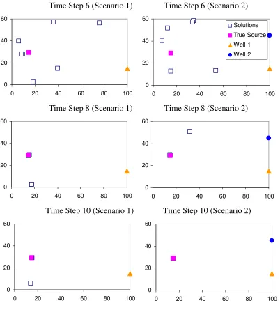
Preliminary results are shown for a two-dimensional homogeneous aquifer with the contaminant introduced at a single location. Plume is generated assuming advection-dispersion processes in the porous media. Synthetic observations at two monitoring wells through 20 time steps are generated assuming a pulse source. Source identification Scenario 1 represents a case wherein a new observation at only Well 1 is incrementally added at each time step. Scenario 2 represents a case wherein new observations at both Wells 1 and 2 are incrementally added at each time step.

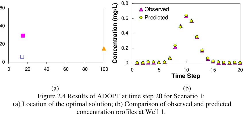
The EA-based ADOPT was executed for 30 random trials for each scenario. The representative results shown here are based on a typical run. For each scenario, the progression of the search procedure is shown in terms of the non-unique solutions obtained for each scenario as more measurements are added over time that is represented by the number of time steps in Figure 2.4. The true source is also shown for comparative purposes.

Parameter Value

Field size 100 m × 60 m

Number of time steps 20

Time step size (∆t) 10 day

Grid spacing (∆x=∆y) 2 m

Dispersion parameters αL=1 m; αT = 1 m; Dm = 0.01 m2/d

Flow field Homogeneous

Velocity 1 m/day

True source description Shape: square (with side length of 2 m) Centroid coordinate: (15, 29)

(35)

Time Step 6 (Scenario 1) Time Step 6 (Scenario 2)

0 20 40 60

0 20 40 60 80 100

0 20 40 60

0 20 40 60 80 100

Solutions

True Source

Well 1

Well 2

0 20 40 60

0 20 40 60 80 100

0 20 40 60

0 20 40 60 80 100

0 20 40 60

0 20 40 60 80 100

0 20 40 60

0 20 40 60 80 100

(36)

0 0.2 0.4 0.6 0.8

0 5 10 15 20

Time Step

C

o

n

c

e

n

tr

a

ti

o

n

(

m

g

/L

)

Observed Predicted

0 20 40 60

0 20 40 60 80 100

(a) (b) Figure 2.4 Results of ADOPT at time step 20 for Scenario 1:

(a) Location of the optimal solution; (b) Comparison of observed and predicted concentration profiles at Well 1.

(37)

additional observations from Well 2 help resolve the non-uniqueness and identify the source correctly.

0 5 10 15 20 25

5 7 9 11 13 15 17 18

Time Step

N

u

m

b

e

r

o

f

s

u

b

p

o

p

u

la

ti

o

n

s

Scenario 1

Scenario 2

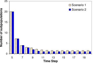
Figure 2.5. Average number of the remaining subpopulations through time.

(38)

2.4. Conclusions and Future Work

This study introduces an adaptive dynamic optimization procedure based on EAs for solving dynamic optimization problems. Whereas the continually shifting optima challenge EAs, ADOPT is designed not only to capture the current optima, but also to simultaneously preserve an appropriate degree of diversity. To arrive at a balance between convergence and diversity, the emphasis is put on either the distance or the objective function in the selection process, which depends on the feasibility of the majority of the individuals in a subpopulation. Such balance ensures the necessary clustering of subpopulations around maximally diverse potential solutions depending on the current status of a problem, the number of subpopulations is dynamically adjusted. This ability could be helpful in improving the solution quality as well as avoiding unnecessary computational costs.

(39)

that the degree of non-uniqueness in solutions varies over time. The results presented here demonstrates that ADOPT has the potential to dynamically identify a set of solutions that yields similar and good fit to the observed data. By varying the observations, either by utilizing longer observation periods or by incorporating more monitoring wells, ADOPT is demonstrated to be successful in adaptively reducing the number of subpopulations and assessing the degree of non-uniqueness.

(40)

CHAPTER 3: Adaptive Contamination Source Identification

in Water Distribution Systems Using an Evolutionary

Algorithm-based Dynamic Optimization Procedure

Abstract. Accidental drinking water contamination has long been and remains a

(41)

information; consequently, several solutions may predict the observations similarly well. To address non-uniqueness in the initial stages of the search and prevent premature convergence of the EA to an incorrect solution, the multiple populations in the proposed methodology are designed to maintain a set of alternative solutions that represent various non-unique solutions. As more observations are added, the EA solutions not only migrate to better solution states, but the number of solutions decreases as the degree of non-uniqueness diminishes. This new dynamic optimization algorithm adaptively converges to the solutions that best match the observations available at any time. The new method is demonstrated for contamination source identification problems in two example water distribution networks.

3.1. Introduction

(42)

observations of the models at the sensor nodes in the network. In the context of a quickly evolving contamination event in a WDS, the correct source characterization must be resolved rapidly as the sensor observations, i.e., contaminant concentrations at the sensors in the network, stream in over time.

Although inverse modeling has been applied to a wide array of system identification problems in engineering, it has the potential for non-uniqueness in that different sources with significantly different pollutant release characteristics but with similar prediction errors may be identified. Because the non-uniqueness in a system is related to the amount of data available for identifying the source(s) of the contamination, more data, made available through either additional sensors or an extended monitoring time, may help reduce the degree of non-uniqueness in the system. If the available information is insufficient to determine whether an identified solution is unique or not, then it is important to determine if other possible solutions exist. Knowing that the identified solution is the only possible source characteristic that matches the observations is critical, because a non-unique but incorrect solution may yield potentially costly mitigation actions that may inconsequentially exacerbate the contamination.

(43)

degree of non-uniqueness, i.e., whether more than one solution fits the available observations.

Recently, researchers have reported the development of several procedures to identify contaminant source characteristics by using information from sensor networks. A direct sequential technique, reported by van Bloemen Waanders et al. (2003), has been applied to solve a small-scale optimization problem using a standard successive quadratic programming tool. Laird et al. (2005) report a direct simultaneous approach. These methods attempt to identify a single solution using a fixed, i.e., not dynamically streaming, set of observations. New approaches are needed to solve the problem in an adaptive manner. At any given time, the procedure must be able to identify possible solutions that explain the observations available up to that time. Also, the solution procedure must identify not only the best estimate of the source characteristics that minimize the prediction error, but also identify a set of possible alternative solutions, if any, that similarly predicts the available observations.

(44)

this chapter is based on EA that is coupled with an EPANET model of the water distribution network. The applicability of the method is illustrated using a hypothetical example.

3.2. Contaminant Source Identification Problem Description in a WDS

To capture the dynamic nature of the available observation data, the source identification problem is described in terms of the source characteristics, based on observations up to the current time. As the number of observations changes over time, the description of the problem is updated at some regular time interval, i.e., the observation frequency. At any instant, the problem can be solved to obtain an estimate of the source characteristics that best explain the currently available data. The following mathematical model is defined to determine, at any given time after the contamination is detected at one or more sensors, the contamination source location, the contamination event start time, and the corresponding contaminant mass loading history. Although the definition provided below assumes that the contamination is introduced at only one node in the network, the proposed approach can be updated to consider multiple contamination source locations.

Find {L,

c t

M , T0}

Minimize c s t t t N i t it obs it t N T M L C C F c s c * )) , , ( ( 0 1 2 0

∑∑

= = −

= , (3.1)

where F = prediction error;

L = contaminant source location;

(45)

t0 = time of first detection of contamination at sensors; tc= current time step;

c t

M = contaminant mass loadings represented as a vector of mass injected at the source from time T0 to tc; Mt_c ={mT₀,mT₀+1,L,mt_c};

obs it

C = observed concentration at sensor i at time step t;

) , ,

(L M T₀ C

c t

it = model estimated concentration at sensor i at time step t;

i = observation (sensor) location;

t = time step of observation; and

Ns = number of sensors.

3.3. Solution Approach

(46)

and Walters, 1997). Although EAs can be used effectively to solve inverse problems, such as WDS calibration (e.g., Vitkosvsky et al., 2000; Lingireddy and Ormsbee, 2002) and groundwater source contamination identification problems (e.g., Mahinthakumar and Sayeed, 2005; Mahar and Datta, 1997), the applicability of EAs to dynamic source characterization in water distribution networks has not been fully investigated. Thus, in this chapter EAs are investigated as an approach to solve adaptively the source determination problem in water distribution networks that is posed as a dynamic optimization model (Eq 3.1). This new EA-based approach, called ADOPT – Adaptive Dynamic OPtimization Technique described in Chapter 2 – is a search procedure that is designed for adaptive optimization and considers dynamically varying streams of sensor observations and identifies alternative solutions, if any, to assess the degree of non-uniqueness in the system.

3.3.1 Evolution Strategy for Contaminant Source Characterization

(47)

The ES presents an adaptive capability, particularly in dynamic circumstances, in that it typically adapts its step lengths during the optimization process. The benefit of the ES is its mutative self-adaptation, whereby each individual can be represented as a decision variable along with its mutation step lengths (Yang, 2007). During the course of mutation, the step length, once mutated, is used to create a random vector to mutate its corresponding decision variable. Thus, mutation rate changes based on the quality of individuals instead of using various predetermined values for parameters, such as mutation and crossover rates. The ES has been demonstrated to possess a self-learning capability, even in the dynamic context of an optimization problem (Hoffmeister and Back, 1992).

To identify a contaminant source in a WDS, a search for various characteristics of contaminants, such as location, starting time, duration, and injection rates at different time intervals is required. The injection profile is represented as an array of real variables, and the source location, starting time, and duration are encoded as integer values in this study. The mutation step size is encoded in a similar way to its corresponding decision variable. The fitness representing the prediction error of an individual is updated with increasingly available sensor observations. Because the mutation operator plays a key role in maintaining diversity within the ES, several mutation strategies to enhance performance were investigated in this study.

3.3.2 Conceptual Basis for ADOPT

(48)

distribution network problem, the number of sensor observations varies with time. That is, the objective function (i.e., the prediction error defined in Eq. 3.1) changes with time. The dynamic optimization procedure is structured to continually search for the best solution at each time step, t. Initially (i.e., at t0 when the contaminant is first detected), the search uses a

set of random solutions as the starting point for the search. The solutions that are found to best fit the observations up to the previous time step are used as the starting solutions for the subsequent instance of the problem that, in turn, is updated with the new observation data obtained during the next observation time step. This approach works well for a population-based search procedure, such as EAs, where the population of solutions continually explores the decision space and migrates towards the right solution as the objective function is adjusted dynamically based on updated observation information over time.

(49)

3.3.3 Algorithmic Steps of ADOPT

(50)

also reveal other possible solutions, if any, to indicate the uniqueness of the solution. The steps of this procedure are listed below.

Step 1. Create an initial set of random solutions, equally divided among N subpopulations.

Step 2. Increment time step t t + 1. Set generation index as g = 0. Update the monitoring data with additional measurements and construct the prediction error function.

Step 2.1. Increment generation index g g + 1. In the first subpopulation (p = 1), evaluate the fitness based on the prediction error. In subpopulation p ( = 2, 3,…N), evaluate the fitness based on the prediction error and its distance from all other subpopulations.

Step 2.2. In each subpopulation, apply selection, recombination and mutation operators, and create a new set of solutions.

Step 2.3. If the stopping criteria (e.g., g < max no. of generations) are not met, then go to Step 2.1; otherwise, go to Step 3.

Step 3. Eliminate subpopulations that represent duplicate solutions. If only one subpopulation remains, or the current set of solutions is acceptable, then stop. Step 4. If no more observations are available, then stop; otherwise, go to Step 2.

3.4. Illustrative Case Studies

(51)

exhibit the ability of ADOPT to predict alternative source characteristics by coupling the EPANET model with the ADOPT search procedure. Specifically, the search is conducted to determine, at the end of each observation interval, a set of source characteristics that includes the location, start time, and mass loading profile of the contaminant as the contaminant is introduced into the network. Also, the sensitivity of the proposed approach to a range of parameter settings and contamination scenarios is investigated.

Upon confronting a contamination event, ES-based ADOPT starts to execute with a prespecified number of subpopulations. Over time these subpopulations are adaptively regulated, according to the sensor observations, to track of the best solution and a set of alternatives. The resultant alternative solutions must perform similarly well in terms of the prediction error, but are maximally far apart from each other. Given these sensor observations, alternatives can be determined according to the currently available data. For example, the target value, which is used to evaluate the feasibility of the solutions, is set to a relaxation value (120% in this study) of the root mean square of the observed data. Considering that the degree of non-uniqueness diminishes as more measurements are collected, the relaxation value is adjusted accordingly (by 0.7% in this study, based on a set of trials). To avoid unnecessary computational costs, a subpopulation is eliminated from the optimization process when it converges to the same location as another subpopulation. The algorithm terminates when the number of remaining subpopulations equals one or when no additional data are monitored.

(52)

each hour. These assumptions are made primarily to allow a convenient and viable investigation and exploration of the proposed approach; however, they are not expected to limit a broader applicability of the approach to problems whose conditions deviate from these assumptions. Table 3.1 describes the allowable ranges of source parameters for both case studies.

Table 3.1 Allowable Range of Source Parameters for the Case Studies

Source Parameter Small Example Micropolis Example

Location Any node (1~97) Any node (1~1575)

Starting Time (hr) 0~4 0~30

Duration (hr) 0~5 0~7

Mass Injection Rate (g/min) 0~30 0~30

3.4.1 Small Example Network

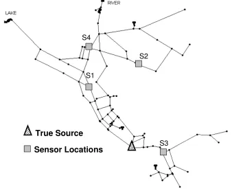
The first network examined is one of the examples available as a tutorial within EPANET (Rossman, 2000). The network is depicted in Figure 3.1, and further details can be found in the EPANET users’ manual. This network consists of 97 nodes, including 2 sources, 3 tanks, and 117 pipes. Four sensors are distributed randomly in this network (denoted as S1, S2, S3, and S4 in Figure 3.1). The contaminant transport is simulated in 10-minute intervals, and the concentration values at the sensors are assumed to be observed in 10-minute increments.

(53)

trials under different contamination scenarios, this scenario was selected as a base run because the pollutant injected at this location seems to be relatively difficult to identify.

S1 S4

S3 S2

Sensor Locations True Source

S1 S4

S3 S2

Figure 3.1 Layout of the small network. Contaminant source for the base scenario is indicated by the triangle. The sensor network is composed of S1, S2, S3 and S4, which are

designated by squares.

(54)

minutes on the Neptune system(an Opteron cluster) where EPANET simulations were executed in parallel on ten processors.

(55)

Figure 3.2 Results for the base scenario using ES-based ADOPT: (a) locations of alternatives at 3:40 a.m. ( the number adjacent to a solution represents the node ID); (b) locations of

(56)

(57)

0 2 4 6 8 10 4:00 AM 5:00 AM 6:00 AM Time C o n c e n tr a ti o n ( m g /L ) Observed Calculated Series3 0 5 10 15 20 25 30 35 2:00 AM 3:00 AM 4:00 AM 6:00 AM Time M a s s I n je c ti o n R a te ( g /M in ) True Calculated Series3 19 7 18 5 19 1 18 7 18 4 20 4 20 6 27 5 20 5 20 7 0 5 10 15 20 25 30 35 2:00 AM 3:00 AM 4:00 AM 6:00 AM Time M a s s I n je c ti o n R a te ( g /M in ) True Calculated Series3 19 7 18 5 19 1 18 7 18 4 20 4 20 6 27 5 20 5 20 7

(c) (d)

Parameter Settings. The proper setting of the algorithm parameters enhances the

effectiveness of discovering solutions. In this section, the sensitivity of the results is evaluated in terms of the differences in the parameter settings for the mutation operators, number of subpopulations, and generation numbers. All experiments were performed for 30 random trials based on the base scenario described above. All the results are reported in terms of the average and one standard deviation (the error bar in the bar charts below) values computed from the solutions obtained for all random trials.

(58)

region in the case of a static situation. Although the ES has been shown to possess a self-learning property in a dynamic environment (Hoffmeister and Back, 1992), more time may be needed to self-adjust step sizes to proper magnitudes from small values than to reinitialize them once an environmental change occurs. As a result, the reconstruction of mutation step sizes may facilitate the adaptability in the dynamic context of the contaminant source characterization.

(59)

the changing environment. To better understand ways that ADOPT performs under different mutation strategies, the level of non-uniqueness represented by the number of alternatives (Figure 3.3(b)), and the number of remaining subpopulations (Figure 3.3(c)) that represents the convergence of individuals as well as the computational cost were compared. As shown in Figure 3.3 (b), the number of alternatives generated provides further evidence for the information presented in Figure 3.3 (a) that the third strategy surpasses the other two schemes. Figure 3.3 (c) reveals a diminishing rate of decline in the number of subpopulations as the sensor observations increase. This trend is more significant in the first experiment due to the lowest of the degrees of diversity introduced during the search process.

0 0.02 0.04 0.06 0.08 0.1

30 60 90 120 150

Time Elapsed (min)

M in im a l P re d ic ti o n E rr o r (m g /L ) Self-adaptation Random mutation Self-adaptation+Re-initialization 0 5 10 15 20

30 60 90 120 150

N u m b e r o f A lt e rn a ti v e s _{Self-adaptation} Random mutation Self-adaptation+Re-initialization 0 5 10 15 20 25

30 60 90 120 150

N u m b e r o f S u b p o p u la ti o n s Self-adaptation Random mutation Self-adaptation+Re-initialization (a) (c) (b) 0 0.02 0.04 0.06 0.08 0.1

30 60 90 120 150

M in im a l P re d ic ti o n E rr o r (m g /L ) Self-adaptation Random mutation Self-adaptation+Re-initialization 0 5 10 15 20

30 60 90 120 150

N u m b e r o f A lt e rn a ti v e s _{Self-adaptation} Random mutation Self-adaptation+Re-initialization 0 5 10 15 20 25

30 60 90 120 150

N u m b e r o f S u b p o p u la ti o n s Self-adaptation Random mutation Self-adaptation+Re-initialization (a) (c) (b)

(60)

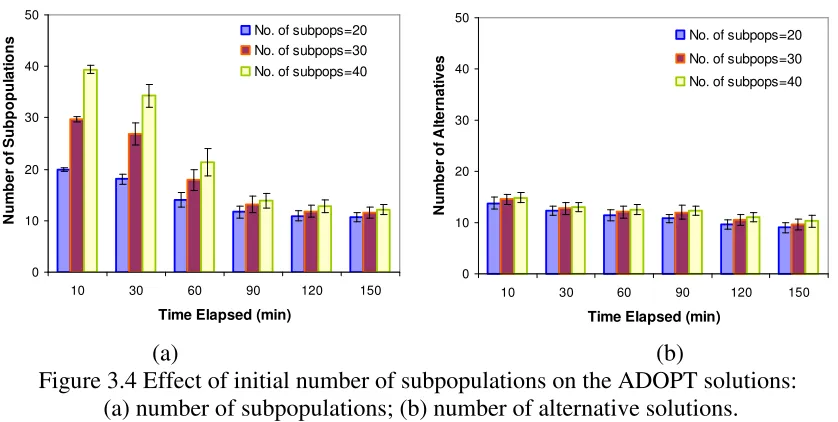
When solving a contamination event using ADOPT, it is desirable for the number of subpopulations to be the same as the number of alternative solutions. It is difficult, however, to predetermine the exact number, and therefore an estimate must be specified to execute the procedure. Sensitivity of the performance of ADOPT to this parameter, the initial number of subpopulations, was conducted for 20, 30, and 40. Figure 3.4 (a) shows the number of subpopulations at different elapsed times for three scenarios. As expected, ADOPT, with more subpopulations converges much faster, but at the end of the observation period (150 mins), similar numbers of subpopulations were reached. Moreover, the initial settings of their numbers do not make much difference to the alternatives identified by ADOPT (see Figure 3.4 (b)). 0 10 20 30 40 50

10 30 60 90 120 150

N u m b e r o f A lt e rn a ti v e s

No. of subpops=20 No. of subpops=30 No. of subpops=40

0 10 20 30 40 50

10 30 60 90 120 150

N u m b e r o f S u b p o p u la ti o n s

No. of subpops=20 No. of subpops=30 No. of subpops=40

(a) (b)

Figure 3.4 Effect of initial number of subpopulations on the ADOPT solutions: (a) number of subpopulations; (b) number of alternative solutions.

(61)

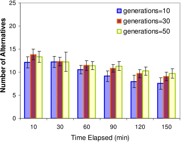
solutions in terms of the objective value at any elapsed time, but compromises diversity or becomes mired in local optima. The over-convergence impacts current solutions as well as subsequent searches, especially at the initial stages when the observations are limited. Because of the loss of individual diversity, further effort is required to adapt solutions once new data become available.

(62)

0 5 10 15 20 25

10 30 60 90 120 150

Time Elapsed (min)

N u m b e r o f A lt e rn a ti v e s generations=10 generations=30 generations=50

Figure 3.5 Effect of the number of generations on the ADOPT solutions.

Various Contamination Scenarios. While the results from the base scenario indicate

the effectiveness of ADOPT in characterizing a WDS contaminant source, a range of contamination scenarios presented here allows the demonstration of the algorithm’s robustness given the variations in the amount and quality of the monitoring data as well as the contaminant source characteristics.

(63)

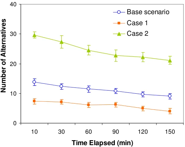
existence of contamination rather than the concentration value. A fixed concentration value specifies the threshold or detection limit to trigger a contamination detection status. A reading that exceeds this threshold (a value of 0.1 mg/L is assumed in this study) represents the presence of contamination (converted to an output signal of 1); otherwise, it represents the absence of contamination (represented by an output signal of 0). The degree of non-uniqueness is measured in terms of the number of alternatives. Figure 3.6 shows comparisons of the number of non-unique solutions identified for the two cases and the base scenario. The degree of non-uniqueness diminishes as the amount of observations increases. In all three scenarios, a decrease in either the number or quality of the sensors leads to a higher degree of non-uniqueness in the solutions.

0 10 20 30 40

10 30 60 90 120 150

N

u

m

b

e

r

o

f

A

lt

e

rn

a

ti

v

e

s

Base scenario Case 1

Case 2

(64)

The behavior of the ADOPT-based approach to different contamination events with various contaminant characteristics was then investigated. Four contamination events were simulated, differing in the injection location, starting time, duration, and/or mass injection rates. A description of the four scenarios is provided in Table 3.2. Figure 3.7 shows the injection locations of the four scenarios as well as the base scenario.

Table 3.2 True Source Description for Four Contamination Event Scenarios

True Source Scenario 1 Scenario 2 Scenario 3 Scenario 4

Location Node 125 Node 105 Node 267 Node 171

Starting time 2:30 a.m. 3:00 a.m. 3:00 a.m. 2:30 a.m. Mass Loading

(g/min)

{15, 20, 25} {10, 20, 25, 25, 15, 10}

{10, 20, 25, 25, 15, 10}

{5, 20, 25, 20, 15, 20, 15, 10, 10 } Duration

(min)

30 60 60 90

105

267

171 125

205(base)

105

267

171 125

205(base)

Figure 3.7 Four hypothetical contamination scenarios along with the base scenario: Contaminant source is indicated by the triangles; the number adjacent to the node represents

(65)

The results of the four scenarios compared to the base run are shown in Figure 3.8. The observations were sufficient to eliminate the non-uniqueness for the scenarios with the contaminant source at nodes 125 and 105 (Scenarios 1 and 2, respectively). In contrast, a higher level of uncertainty was found for the other scenarios, which is likely due to the true source location in relation to the sensor locations in the network. It is also noted that for the contaminant introduced at nodes 125, 105, and 267 (Scenarios 1, 2, and 3, respectively), the true source node is always identified as one among the alternative set, whereas for the source at nodes 205 (scenario 2) and 171 (scenario 4), the true node is not always among the alternative solutions. With regard to the distribution of the resulting non-unique solutions for all scenarios, most of the solutions are concentrated in the vicinity of the true source, which may be due to the hydraulic similarities among their vicinities. These alternatives gradually move towards the true source node as more measurements become available.

0 5 10 15 20

20 30 60 90 120 150 180

Elapsed Time (min)

N

u

m

b

e

r

o

f

A

lt

e

rn

a

ti

v

e

s

Scenario 1 (#125) Scenario 2 (#105) Scenario 3 (#267) Scenario 4 (#171) Base scenario (#205)

(66)

3.4.2 Micropolis Example Network

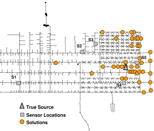
To understand the impact of the increasing level of problem complexities on the alternatives identified by ADOPT, a second network was studied. This relatively large network consists of 1574 junctions, 2 reservoirs, and 1 tank, as illustrated in Figure 3.9. This example was developed for a virtual city with 5,000 residents, further details of which can be found in Brumbelow et al. (2007). The locations of five ideal sensors are randomly selected within the entire network (see Figure 3.9). The contaminant transport is simulated at 10-minute intervals, and the concentration values at perfect sensors are assumed to be observed at each 10-minute increment.

Sensor Locations S1

S5

S4 S3

S2

True Source

Sensor Locations S1

S5

S4 S3

S2

True Source

(67)

(68)

Sensor Locations

S1

S5

S4 S3

S2

True Source

Solutions

Sensor Locations

S1

S5

S4 S3

S2

True Source

Solutions

Figure 3.10 Identified solutions at 6:50 p.m. for the hypothetical contamination event in the micropolis network.

(69)

Sensor Locations S1 S5 S4 S3 S2 True Source Solutions Sensor Locations S1 S5 S4 S3 S2 True Source Solutions

Figure 3.11 Identified solutions at 9:00 p.m. for the hypothetical contamination event in the micropolis network. 0 1 2 3 4 5 6:00 PM 7:00 PM 8:00 PM 9:00 PM Time C o n c e n tr a ti o n ( m g /L ) ObservedCalculated Series3

(70)

From the results of the base scenario in the small network and beginning with a given number of subpopulations, multiple subpopulations efficiently converge to the optimal and alternative solutions. Eventually, the number of remaining subpopulations tends be similar to that of the alternatives. For comparison, Figure 3.13 presents the number of subpopulations and alternatives that vary over time for this example and are averaged over 30 random trials. The results indicate that after the first set of measurements, the remaining subpopulations are much more numerous than the alternatives due to insufficient convergence in the search. This discrepancy in numbers also illustrates the necessity to enhance the algorithm’s efficiency in the face of increasing complexities and limited computational resources.

0 10 20 30 40 50 60 70 80

10 30 60 90 120

N

u

m

b

e

r

Number of subpopulations

Number of alternatives