Gametic Disequilibrium Measures: Proceed With Caution

Gametic Disequilibrium Measures: Proceed With Caution

Philip

W.

Hedrick'

Department of Genetics, University of Calijornia, Berkeley, Calijornia 94 720

Manuscript received February 12, 1987 Revised copy accepted June 20, 1987

ABSTRACT

Five different measures of gametic disequilibrium in current use and a new one based on R. C. Lewontin's D ' , are examined and compared. All of them, except the measure based on Lewontin's

D ' , are highly dependent upon allelic frequencies, including four measures that are normalized in some manner. In addition, the measures suggested by A. H. D. Brown, M. F. Feldman and E. Nevo, and T. Ohta can have negative values when there is maximum disequilibrium and have rates of decay in infinite populations that are a function of the initial gametic array. T h e variances were large for all the measures in samples taken from populations at equilibrium under neutrality, with the measure based on D' having the lowest variance. In these samples, three of the measures were highly correlated, Dz, D* (equal to the correlation coefficient when there are two alleles at each locus) and the measure X(2) of Brown et al. Using frequency-dependent measures may result in mistaken conclusions, a fact illustrated by discussion of studies inferring recombinational hot spots and the effects of population bottlenecks from disequilibrium values.

I T H the advent of new biochemical techniques,

W

it has been possible to distinguish many alleles at a number of loci and to document DNA differences at closely linked sites on a chromosome. If population data from such studies are examined, the extent of the statistical association of the alleles at different loci or sites, gametic disequilibrium, may be an indicator of the past importance of various evolutionary factors. However, these are a variety of gametic disequilibrium measures that have been proposed by different re- searchers.

There are a number of criteria that can be used to determine the most appropriate measure of gametic disequilibrium for a given situation. Several possible criteria are that a measure should have (1) a simple biological interpretation,

(2)

statistical tests available or easily developed, (3) be directly related mathemat- ically to evolutionary factors such as recombination, selection, genetic drift, gene flow, etc. and

(4)

be standardized to allow comparison across loci or pop- ulations. Obviously, all of these criteria (and probably more) are important characteristics for a disequilib- rium measure. In addition, it is not obvious whether different measures gave similar information, or whether different measures may give complementary information.

Below I will examine six different measures of two- locus gametic disequilibrium. First, I have compared some of the basic properties of the different measures focusing on the allelic frequency dependence of the measures and the rate of decay of disequilibrium from

' Permanent address: Division of Biological Sciences, University of Kansas. Lawrence, Kansas 66045.

Genetics 117: 331-341 (October, 1987)

recombination. Second, I have compared the distri- butions of these measures and calculated the correla- tion coefficients between them for a large number of randomly obtained samples.

MEASURES OF GAMETIC DISEQUILIBRIUM

T h e extent of gametic disequilibrium (I use the term gametic disequilibrium instead of the traditional term linkage disequilibrium because such nonrandom association may be present between unlinked loci) [see HEDRICK, JAIN and HOLDEN (1978) for a discussion] can be measured in several ways for a specific gamete. A widely used measure of gametic disequilibrium for a given gamete is

(1) where x, is the observed frequency of gamete AiBj,

pi

and qj are the frequencies of alleles Ai and Bj at loci A and B, respectively, and the expected frequency of gamete AiBj is piqj, assuming no statistical association between the alleles. T h e range of this measure of gametic disequilibrium is a function of the allelic frequencies, making it obvious that a measure that has the same range for all allelic frequencies is desirable. For this reason, LEWONTIN (1964) suggested using the normalized measure

D, = x..

-

p-q.

rj ' I

(2) D!. =

D,.

rj

Dmax

where D,,, = min[piqj, (1

-

pJ(l

-

qj)] when D, 0 or D,,, = min[pi( 1

-

qj), (1 - pi)qj] when D,

>

0.

example, the disequilibrium can be expressed as HOLLAND 1975), the measure

k l

D 2 =

1

2

D$

(3) j = I

where there are K alleles at locus A and I alleles at locus B . However, this measure, like D,, is highly dependent upon allelic frequencies. As a result, other measures of association in which the overall disequi- librium is normalized and not so dependent on allelic frequencies have been suggested.

One such approach is to standardize the measure by the single-locus heterozygosity. For example, the Hardy-Weinberg homozygosity at locus A having

k

alleles is

k

F A =

pt"

I= I

and for locus B with 1 alleles is

I

Fn = .9; (4b)

j= 1

T h e Hardy-Weinberg heterozygosities, H,+ = 1

-

FA and H B = 1

-

F s , can be used in a standardized

measure of two-locus association as

a measure termed R by MARUYAMA (1 982).

loci that

First, note that when there are two alleles at both

D 2

4p1(1 - pi)qI(l

-

41)' (5b) D* =

Because all D, are equal with two alleles at both loci, then D 2 = 405 and D* is equal to the square of the correlation coefficient as used by HILL and RORERT-

SON (1968) and FRANKLIN and LEWONTIN (1970). Second, note that expression (5a) is different from 0% as given by HILL (1975) and OHTA (1980), D * , when calculated over a number of samples, is the mean of the ratio in (5a) whereas ai is the ratio of the means (or expectations), an important difference in many situations (MARUYAMA 1982; HEDRICK and THOMSON 1986, Table 4). Obviously, ai is mathemat- ically more tractable but D* is the experimentally observable quantity in each population or pair of loci

(MARUYAMA 1982).

Another measure of standardized gametic disequi- librium is

(HILL 1975). In order to make this measure sample- size independent when

D

# 0 (BISHOP, FEINBERC and

is useful (HEDRICK and THOMSON 1986). D* and Q* are equal for

K

=

1

= 2. YAMAZAKI (1977) proposed the related measure

where it is assumed that

k

<

E . Because L is a linear function of

e*,

we will not give values for it in the following discussion.

If we define

k 1

F A B =

c

c

x:

i=l , = I (9)

another measure of association is

(10)

F * = FAn

-

FAFB

by OHTA (1980) and is equivalent to the covariance of heterozygosity measure of AVERY and HILL (1979).

OHTA (1 980) suggested F* could be standardized with the product of the Hardy-Weinberg heterozygosities as

This measure is somewhat different from the stand- ardized measure of OHTA (1 980) in that for a number of samples, she uses the mean of F A B , FA and FB over samples to calculate her measure (see discussion of D

*

above).

BROWN, FELDMAN and NEVO (1980) suggested a measure of disequilibrium based on the variance of heterozygosity, higher variance of heterozygosity being the result of higher gametic disequilibrium. If it is assumed that K is the number of heterozygous loci, then for two loci K = 0 for the double homozy- gotes, K = 1 for the single heterozygotes and K = 2 for the double heterozygotes. T h e variance of K for two loci is then

(1 2)

sf = HA

+

Hn

-

H;

-

H i

k 1

+

4

2

2

pIqJ

D ,

+

20' 1 = I 1 = I

where the

2

refers to the second central moment. When there is no disequilibrium, then X(2) = 0.

Finally, the normalized measure of LEWONTIN can also be used for a total disequilibrium measure. For example.

k 1

D ’ =

c

c

piq,

IDhl

(14)

1=1 j = 1

gives values of the absolute value of the normalized D

weighted by the frequencies of the gametes when there is no disequilibrium. A similar measure was used by KARLIN and PIAZZA (1982) but they used xq values for weighting.

GENERAL PROPERTIES

Frequency-dependence: An important characteris- tic of a gametic disequilibrium measure is that it is independent (or nearly independent) of allelic fre- quencies. For example, a measure that is highly de- pendent on allelic frequencies would not be appropri- ate for comparisons between samples or loci with different allelic frequencies. To examine the depend- ence on allelic frequencies of these six measures, let us first assume that there are two alleles at each of the two loci and use DI; as a standard because it is inde- pendent of allelic frequencies. Assuming that there is a given Dl[l value, we can calculate the value of the different measures for various allelic frequencies at the two loci. For example, if D ~ I

>

0 and plq2

<

p241,

then

Dri = D ; I pi42 (15)

and the various standardized measures, D * , Q*, F‘, X(2) and D ’ can then be calculated (remember D * =

Q*

for two alleles). As an example of what the gametic frequencies are for given values, let D

il

= 1,

p l

= 0.1, and 92 = 0.5, then D I I = 0.05, X I I = p1q1

+

D11 = 0.1, x 1 2 = 0.0, x z l = 0.4, and x22 = 0.5. T h e other disequi-

librium measures are then D* =

Q*

= 0.11 1, F’ = 0.1 11, X(2) = 0.030, and

D ’

= 1.0.

Using this approach, the values of D * =

Q*,

F ’ , and X(2) are plotted in Figures 1, 2, and 3, respec- tively, for different allelic frequencies when O i l = 0.5

( D ’ = 0.5 for all allelic frequency combinations).

When D;1 = -0.5, complementary results occur and when ID;ll

<

0.5, then similar but not as extreme results occur. First, notice that all of these measures, even though they are standardized in some manner, are highly dependent upon allelic frequencies. For example, looking at D* = Q* in Figure 1 and X(2) in Figure 3, if one locus has both alleles at intermediate frequency, say q1 = q 2 = 0.5, and the other locus has

one allele in much higher frequency, say

p l

= 0.05

and

p 2

= 0.95, then the calculated values are much

lower than if the alleles at both loci were intermediate in frequency.

0.25

0.20

0.15 b

n

0.10

0.05

0.00

0.0 0.2 0.4 0.6 0.8 1.0

41

FIGURE 1 ,-Magnitude of D* for different p1 and q1 values when D ’ = 0.5.

4.0

3 . 0

L 2.0

1.0

0.0

-1.0

’

I I I I

I

0.0 0.2 0.4 0.6 0.8 1.0

41

FIGURE 2.-Magnitude of F’ for different p l and q , values when D ’ = 0.5.

Second, notice that the maximum values for each measure occur when the allelic frequencies at the two loci are equal. For D* =

Q*,

this maximum is the same for all = q 1 values (Figure 1). However, for

F’ and X(2) the maximum is greatest when the allelic frequencies are low, i.e., F’ and X(2) are large when

$ 1 = q1 = 0.05 (Figures

2

and 3). Furthermore, F’ has

the property that when both

P I

and ql are low it becomes very large, e.g., if

p l

= q1 = 0.01, F’ = 24.5,

compared to when p l = q1 = 0.5, then F‘ = 0.25.

0.5

0.4

[n

0.3

-

0.2

X

0.1

0.0

TABLE 1

Amount of disequilibrium for the different measures when R =

I , and all xi<

=

l/k

k(=l)

~~

2 3 4 k

D 2 0.25 0.222 0.1875

fi

k2

D* 1

.o

0.5 0.333

_-

1

k - 1

Q*

1

.o

0.5 0.333

_-

1

k - 1

F’ 1

.o

0.5 0.333

_-

1

k - 1

X(2) 1.0 1

.o

1

.o

1

D’ 1

.o

1

.o

1

.o

1

-0.1

’

I I I I

I

0.0 0.2 0.4 0.6 0.8 1.0

91

FIGURE 3.-Magnitude of X(2) for different p , and q1 values. when D ’ = 0.5.

THOMSON (1 986) showed that this occurs when there are two alleles at each locus for F* when

-2D(p1q1

-

piqz

-

P H I

+

pzqz)

<

40’. (16)

T h e same conditions are also true for F’ and X ( 2 ) .

T o determine the maximum value of these different measures for given allelic frequencies, expression ( 2 )

with the substitution D ; I = 11

I ,

gives D I I = D,,,.

Substituting the value of D,,, in the various equations gives the maximum possible so, for example, the max- imum D* when DII

>

0 and

P I

(1

-

q1)

<

(1 - p1)qI

becomes

To calculate the maximum F’, expression ( 2 2 ) can be used.

When there are multiple alleles, the disequilibrium is intuitively highest when there are the same number of alleles at both loci

(k

= I ) and xii =

p ,

= qi (all other gametes, xq = 0 where

i

# j ) , a situation termed absolute association by CLEGG et al. (1976). First, assuming only coupling gametes are present in the population and all are at equal frequency, i.e.,

p ,

= qi

= 1/k, then we can calculate the disequilibrium gen- erated for the different measures (see Table 1). In this situation, D* = Q* = F’ = 1/(K

-

1) and the extent of disequilibrium declines for these measures as the number of alleles increases. X ( 2 ) and

D ’

are equal to unity for any number of alleles. T h e depend- ence of D * ,

Q*

and F’ on the number of alleles at a locus makes these measures less useful when compar- ing samples with different numbers of alleles. This problem could be rectified by multiplying them by

k

- 1 when

k

= 1 (remember YAMAZAKI’S measure L does this for Q*).

Second, let us assume that there is still absolute association and only coupling gametes but relax the assumption that all gametes have a frequency of l/k. Table 2 gives the values for the different measures for examples with 2 , 3, and 4 alleles and general expressions for

k

alleles. T h e allelic frequencies chosen for the examples are ones that fit the expectations for a neutrality population with a given number of alleles

(EWENS 19’79). In this case again, X ( 2 ) and

D’

are always unity and

Q*

= l/(k

-

1). O n the other hand,

D * and F

’

do not have values solely dependent on the number If alleles as they did when all coupling ga- metes had equal frequencies.

Given that there are more than t w o alleles at both loci, and the frequencies of the alleles at the two loci are different, i.e., pi # qi, then in general there is no

way in which D ‘ can be unity. However, for three alleles it is possible to have D ’ = 1 given that

P I

2

p2

+

p 3 and q1 2 q 2

+

4 3 . Table 3 (center columns) gives an example of two such gametic arrays with

P I

= 0.5,

p2

= p 3 = 0 . 2 5 and q 1 = 0 . 8 5 , q2 = 0.1, and qs = 0.05

and similar ones given equal allelic frequencies at the two loci

( P I

= q 1 = 0.85,

p 2

= q2 = 0.1, and

p 3

= qs =

0.05 in the left column and $ 1 = q1 = 0.5 and

p 2

=

p s

= q 2 = 4 3 = 0.25 in the right column). First, notice

TABLE 2

Amount of diseguilibrium for the different measures when R(=Z) and there is absolute association with xii

=

pi = qi and the allelic frequencies at a locus differ"

k(=l)

2 3 4 k

(0.92, 0.08) (0.85,0.1, 0.05) (0.79,0.15,0.05, 0.01) ( P I , p2, p3. . .P*)

k k k

0.0217 0.0440 0.0776

c

P W

-

P Y

+

cz

p:p;

1- 1 1 3

02

0 2

D*

Q*

1

.o

1 .o

0.637

0.5

F' 0.173 0.361

X(2) 1

.o

D' 1

.o

1

.o

1

.o

0.630

0.333

0.540

1

.o

1 .O

1

R - 1

-

1

1

The frequencies of the coupling gametes are given in parentheses.

TABLE 3

Amount of disequilibrium for different measures for the gametic arrays given

0.7, 0.1.0.05 0.35,0.1,0.05 0.5, 0.0,O.O 0.0, 0.25,0.25

0.1, 0.0, 0.0 0.25, 0.0, 0.0 0.25,0.0, 0.0 0.25, 0.0, 0.0

0.05,0.0,0.0 0.25,0.0,0.0 0.1, 0.1,0.05 0.25,0.0,0.0

02 0.0012 0.0131 0.0306 0.141

D* 0.0174 0.0792 0.185 0.360

Q* 0.0078 0.044 1 0.132 0.250

F' -0.359 -0.0943 0.358 0.280

X- -0.130 -0.0728 0.277 0.467

D' 1

.o

1

.o

1

.o

1

.o

(2)

~~~~~ ~ ~~ ~ ~ ~~~

then F' and

X(2)

may either be positive or negative depending upon the particular gametic array.

Rate of decay: Another important property of a disequilibrium measure is the rate of decay of dise- quilibrium as indicated by the measure in an infinite or very large population. It is assumed here for sim- plicity that some factor such as a population bottleneck or hybridization of two populations generates some disequilibrium and then the decay of disequilibrium is only a function of the amount of recombination c between the two loci. It is important to note that disequilibrium can be generated continuously by such factors as genetic drift (e.g., HILL and ROBERTSON

1968; OHTA and KIMURA 1969) and selection (e.g.,

LEWONTIN and KOJIMA 1960) and the rate of decay may also be affected by inbreeding, the mode of reproduction, or selection (e.g., HEDRICK 1980; P. W.

HEDRICK, unpublished data, 1987; ASMUSSEN and

CLEGG 1982).

A well known result (e.g., HEDRICK 1983) is that

D f t + l = (1

-

c)Dlj..t. (18)

In other words, the rate of decay per generation is the ratio of the disequilibrium in generation t

+

1 to that in generation t so that for the measure

DU,

the rate of decay is 1

-

c. In addition, because

= (1

-

c)tDy.o (19)

the rate of decay over t generations for the measure

Dg

is (1 - c)~.

Because H A , HB,

pi,

and q, do not change as a result of recombination, then

(204

(20b)

( 2 0 4

( 2 0 4

0:+1 = (1 - C)ZD;'

D 3 ,

= (1

-

C)ZDT

Q31

= (1

-

c)"?

0 : + 1 = (1

-

c)DI and

making the rate of decay per generation for

D 2 ,

D *

and

Q*

equal to (1

-

c)' and that for D' equal to 1

-

c. In addition

0: = (1

-

c)2'D:

D r = (1 - c)"D,*

Q? = (1

-

C y Q ;

Dl

= (1

-

C)tDG

(214

(2 1 b)

(2 1 4

TABLE 4

Rate of decay per generation for F‘ and X ( 2 ) when there is absolute association of alleles (only coupling gametes)

~- k ( = l )

2” 3” 4“

p. = I l k and/or

Generation q,= 1/1 c = 0.05 c = 0.5 c = 0.05 c = 0.5 c = 0.05 c = 0.5

1 ( 1

-

c)’ 0.942 0.457 0.939 0.443 0.934 0.415

2 0.942 0.476 0.940 0.467 0.934 0.449

3 0.942 0.488 0.940 0.483 0.935 0.471

4 0.943 0.494 0.940 0.491 0.935 0.485

5 0.943 0.497 0.941 0.495 0.936 0.492

10 0.944 0.499 0.942 0.500 0.938 0.500

20 0.946 0.945 0.942

40 0.949 0.948 0.947

80 0.950 0.950 0.950

Asymptotic (1 - c)’ (1

-

4 (1 - 4 (1

-

4 (1 - 4 (1 - 4 (1 - 4

T h e initial gametic arrays used here were the same as in Table 2.

TABLE 5

Rate of decay per generation for F’ and X ( 2 ) for the four initial gametic arrays given in Table 3 when e = 0.05 or 0.5

Generation

1 2 3 4, 5 10 20 40 80 Asymptotic

0.05 0.5 0.05 0.5 0.05 0.5 0.05 0.5

0.952 0.952 0.952 0.952 0.952 0.951 0.951 0.950

(1 - c )

0.5 12 0.506 0.503 0.501 0.501 0.500

0.990 0.710 0.986 0.574 0.983 0.532 0.980 0.515 0.978 0.507 0.969 0.501 0.960

0.953 0.950

(1 - c ) (1 - E )

0.926 0.371 0.926 0.413 0.927 0.447 0.927 0.471 0.928 0.484 0.931 0.499 0.936

0.944 0.950

(1

-

4

(1 - c )

0.889 0.179 0.888 0.050

0.886 0.82 0.885 0.598 0.878 0.504 0.842 0.500 1.024

0.954

0.887 -1.750

(1

-

c) (1

-

c)

making the extent of decay for

D’,

D * ,

and Q* over t generations equal to ( 1

-

c)” and that for D’ equal

T h e rates of decay for F’ and X ( 2 ) are more com- plicated than the other measures but equal to each other. T h e basis for their equivalent rate of decay can be seen when x, =

D,

+

p2qJ is substituted [from

expression ( I ) ] into expression (1 0) which then be- comes

F* = D 2 + 2 c

to (1 - c y .

k l

plq,

D,

(22)

r = l ,=I

k I

+

i

f:

p:q:

-

c

p;”

c

9:.

2=1 ,=I 2 = 1 , = I

Notice that expressions ( 1 2 ) and ( 2 2 ) both have dise- quilibrium measures of the same sort and ratio, D’ to

2C&q,D,, indicating the reason for the same rate of

decay for these measures. Of course, terms composed only of

p ,

and q, combinations do not change as the result of recombination.

Because both F’ and X ( 2 ) are functions of both

D 2

and D,, their rate of decay is a function of the initial

gametic array. To illustrate their behavior, some ex- amples are given in Tables 4 and 5. First, note in the first column of Table 4 that when all

p t

= l/k and/or all q, = 1/Z that the rate of decay per generation for

F‘ and X ( 2 ) is (1

-

c)’just as it is for

D 2 ,

D* and Q*. Second, in the remainder of Table 4 assuming still absolute coupling but unequal allelic frequencies, then the rate of decay changes but eventually asymptotes at 1 - c. In other words, with initial absolute disequi- librium the per generation rate of decay may be ( 1

-

c)’ or (1

-

E ) depending upon the initial gametic array.

Finally, in Table 5 the rate of decay is given for the arrays in Table 3. Here, all the arrays eventually have a decay rate of I

-

c but some start out in the early generations with a much slower decay rate, e.g., array ( b ) , while others have a much faster decay rate, e.g.,

Gametic Disequilibrium

TABLE 6

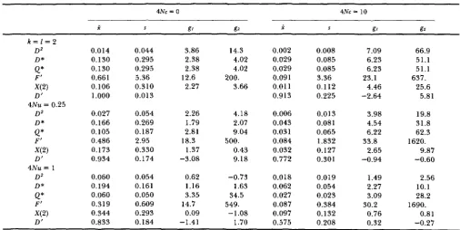
Statistics describing the distribution of six measures of total disequilibrium for n = 200

337

k = 1 = 2

D 2 D*

Q*

F‘ X(2) D‘ D 2 D*

Q*

F’ X(2) D’

4Nu= 1

D Z D*

e*

F’ X(2) D’

4Nu = 0.25

0.014 0.130 0.130 0.661 0.106 1

.ooo

0.027 0.166 0.105 0.486 0.173 0.934 0.060 0.194 0.060 0.319 0.344 0.833 0.044 0.295 0.295 5.36 0.310 0.013 0.054 0.269 0.187 2.95 0.330 0.174 0.054 0.161 0.050 0.609 0.293 0.184 3.86 2.38 2.38 2.27 12.6 2.26 1.79 2.81 1.37 18.3 -3.08 0.62 1.16 3.35 0.09 -1.41 14.7 14.3 4.02 4.02 3.66 200. 4.18 2.07 9.04 0.43 9.18 -0.73 1.63 34.5 -1.08 1.70 500. 549. 0.002 0.029 0.029 0.091 0.01 1 0.913 0.006 0.043 0.031 0.084 0.032 0.772 0.018 0.062 0.027 0.087 0.097 0.575 0.008 0.085 0.085 3.36 0.112 0.225 0.013 0.081 0.065 1.832 0.127 0.301 0.019 0.054 0.023 0.384 0.132 0.208 7.09 6.23 6.23 23.1 4.46 -2.64 3.98 4.54 6.22 33.8 2.65 -0.94 1.49 2.27 3.09 0.76 0.32 30.2 66.9 51.1 51.1 25.6 637. 5.81 19.8 31.8 62.3 1620. 9.87 -0.60 2.56 10.1 28.2 1690. 0.81 -0.27

for one generation, then a large positive value, and finally asymptotes to 0.5.

SIMULATION TECHNIQUES

In order to compare the overall values of these measures in an objective manner rather than for se- lected examples, random samples were obtained using the program of HUDSON (1983). These samples are of a specified size n from a population under neutrality equilibrium where N is the finite population size, U is

the mutation rate to new alleles, and c is the recom- bination rate between the two loci. T h e samples were examined both conditioned on the number of alleles at the A locus

(k)

and the B locus ( I ) and uncondition- ally, i.e., for all samples obtained from a given param- eter set of 4Nu and 4Nc. T h e conditional samples used were all larger than 1,000 while the unconditional samples were between 10,000 and 20,000. T h e results conditioned on allele number will focus on

k

= 1 =

2,

the form in which most restriction site or base poly- morphism data is generally observed. From extensive simulations, HUDSON (1985) has shown that for a sample from a neutrality population the disequilib- rium values, conditioned on the number of alleles, are nearly independent of 4Nu.

Distributions of measures: HEDRICK and THOMSON (1986) discussed at length the distribution of the disequilibrium measures, D

*,

Q* and F

*,

conditioned on the number of alleles in a sample of size n , giving the mean, 95% intervals as well as the distributions of F* and Q* for a particular combination of parameters.

One general conclusion from this examination was that these distributions generally have very large var- iances so that the 95% interval in the cases of D* and Q* extended from the minimum of zero to a quite large value. In addition, these measures all appeared to be right-skewed, i.e ., having long tails of high disequilibrium values. T h e 95% intervals were re- duced as the number of alleles in the sample increased and as 4Nc became larger. T h e unconditional distri- bution of D* was examined by MARUYAMA (1 982) and he found that it had a large variance with a long right- hand tail. If 4Nc is small, say <O. 1, then the distribu- tion is slightly U-shaped because some samples are at maximum disequilibrium [see Figure 5 in MARUYAMA (1982)l. Both GOLDINC (1984) and HUDSON (1985) investigated the conditional distribution of disequilib- rium when there are only two alleles at each locus.

With this background, let us examine some of the distributional properties of the six different disequilib- rium measures given above. As an overall perspective, Table 6 gives the distributional properties for samples of size 200 conditioned on

k

= 1 = 2 and unconditioned for 4Nu = 0.25 and 1 when 4Nc = 0 and 10. T h e statistics used are the mean ( i ) , standard deviation (s) and

gl

and gz, measures of skewness and kurtosis, respectively, that have expectations of zero when the distribution is normal (e.g., SOKAL and RHOLF 198 1). First, let us compare

D2,

D * , Q*, and X ( 2 ) , a group of measures that we will find below to be generally highly correlated with each other. In fact, Q* is cor- related only when

k

and 1 are low, remember when

k

338 P.

0.10 r

0.08

)r 0.06

U

c

W

z

I= 0.04

0.02

0.0 0.1 0.2 0.3 0.4 0.5 0.6’0.6

x (21

FIGURE 4.-Distribution of X ( 2 ) when n = 200, 4Nc = 10 and 4 N u = 1 .

the standard deviation is the same general size as the mean or larger, indicating the extreme variance of these distributions. Note that when

k

= I = 2 the standard deviation of these four measures is much larger than the mean. Second, these measures show right skewness (positive g1 values) with the largest g l

values for

Q*

and D*. In other words, these measures have a few samples with much higher than the average disequilibrium, particularly for larger 4Nc values. Last, these measures generally have flatter distribu- tions than normal distributions, i.e., platykurtic with positive g2 values, a characteristic that is more pro- nounced for higher 4Nc values. Overall, X ( 2 ) is the measure of these four that is the least right-skewed and platykurtic, i.e., the measure of these four having the most normal distribution.

T h e distributions of

D*

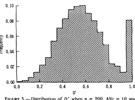
and Q* conditioned on sample size are similar to the distributions conditioned on both sample size and allele number and given in HEDRICK and THOMSON (1 986). As an example of the distribution for X(2), its distribution is given for 4Nu = 1, 4Nc = 10, and n = 200 in Figure 4 . T h e 95% interval extends from 0.002 to 0.392, with a few values larger than 0.6.

T h e other two measures, F’ and D’, are different because F’ can have very extreme values when HAHB is low and D

’

is a function of the normalized measure

05. For example, notice that the mean value of F’ is larger for 4Nu = 0.25 than for 4Nu = 1.0. T h e extreme right skewness and platykurtosis of F’ is the result of these occasionally large F’ values. D’ has a smaller standard deviation relative to its mean than does the other five measures. T h e mean of D’ is relatively near the maximum of unity for all cases in Table 6 except 4Nc = 10 and 4Nu = 1, and generally it shows a left skewness. In other words, when 4Nu =

0.25 and 4Nc = 0, most of the D’ values are quite high but an occasional sample has low disequilibrium

0.10

0.08

5 0.06 c

W

3

F

0.04

0.02

n M ”. -”

0.0 0.2 0.4 0.6 0.8 1.0

0‘

FIGURE 5.-Distribution of D ’ when n = 200, 4Nc = 10 and

4Nu = 1 .

as measured by D’, giving the left skewness. Figure 5 gives the distribution of D’ when n = 200, 4Nc = 1 and 4Nu = 1. Notice the symmetry of the distribution of D’ if the D

’

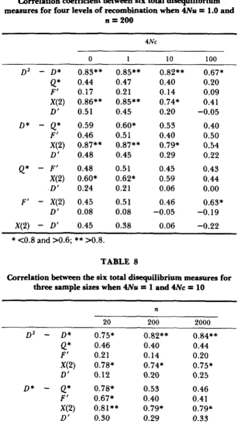
= 1 .O class is ignored, suggesting that along with X(2) that D’ is the most normally distrib- uted of the measures.

Correlation of measures. T h e pairwise correlation coefficients of the six different total disequilibrium measures was calculated for samples from a population at equilibrium under neutrality for a wide range of values of n, 4Nu and 4Nc. First, let us examine the correlation coefficients for a range of recombination values (keeping 4Nu and n constant) because we know that the disequilibrium values decrease as 4Nc in- creases (Table 6). One way to evaluate the pattern of these correlations is to focus on values above a given magnitude. As a guide, the correlations above 0.8 and between 0.6 and 0.8 are indicated in Table

7

(and subsequent tables).

First, note that in general the magnitude of the correlation between any given pair of measures, par- ticularly the pairs with high correlations, declines as 4Nc increases. T h e major difference occurs between 4Nc = 10 and 4Nc = 100, suggesting that for the range between 4Nc = 0 and 4Nc = 10 (and maybe somewhat larger), the correlation patterns are consist- ent. T h e highest correlations are between the meas- ures D 2 ,

D*

and X(2). If we look at the values of 4Nc = 0, 1, and 10, all of the correlations between these measures are above 0.6 and

7

of 9 are above 0.8. In other words, these three measures form a group that appear to give much the same information concerning disequilibrium.

Disequilibrium

TABLE 9

TABLE 7

Correlation coefficient between six total disequilibrium measures for four levels of recombination when 4Nu

=

1.0 and

n = 2 0 0

Correlation coefficient between the six total disequilibrium measures for three levels of mutation when 4 N c

=

10 and n

=

200

4Nc

0 1 10 100

D 2

-

D*

F'

D'

D *

-

Q*

F'

D'

Q*

-

F'

.D'

D' X(2)

-

D'

Q*

X(2)

X(2)

X(2)

F'

-

X(2)

0.83** 0.44 0.17 0.86** 0.51 0.59 0.46 0.87** 0.48 0.48 0.60* 0.24 0.45 0.08 0.45 0.85** 0.47 0.21 0.85** 0.45 0.60* 0.5 1 0.87** 0.45 0.51 0.62* 0.21 0.51 0.08 0.38 0.82** 0.40 0.14 0.74* 0.20 0.53 0.40 0.79* 0.29 0.45 0.59 0.06 0.46 -0.05 0.06 0.67* 0.20 0.09 0.41 -0.05 0.40 0.50 0.54 0.22 0.43 0.44 0.00 0.63* -0.19 -0.22

*

<0.8 and >0.6;

**

>0.8.

TABLE 8

Correlation between the six total disequilibrium measures for three sample sizes when 4Nu

=

1 and 4 N c = 10

n

20 200 2000

Q* 0.46 0.40 0.44

F' 0.21 0.14 0.20

X(2) 0.78* 0.74* 0.75*

D' 0.12 0.20 0.25

D *

-

Q* 0.78* 0.53 0.46

F' 0.67* 0.40 0.41

X(2) 0.81** 0.79* 0.79*

D' 0.30 0.29 0.33

Q*

-

F' 0.76* 0.45 0.38

X(2) 0.74* 0.59 0.57

D' 0.13 0.06 0.06

F'

-

X(2) 0.65* 0.46 0.55

D' 0.03 -0.05 -0.09

X(2)

-

D' 0.04 0.06 0.07

D 2

-

D * 0.75* 0.82** 0.84**

*

<0.8 and >0.6;

**

>0.8.

low correlations with the other measures and with each other (no values above 0.6).

Second, let us examine the effect of different sample sizes on the correlation coefficient for given

4Nu

and 4Nc values. Table 8 gives these correlations for a 100- fold range in sample size from n = 20 to n = 2000. Notice again

D2,

D * ,

and X ( 2 ) form a cluster of high values with

Q*

being slightly lower. Importantly, the correlations between the measures in the high cluster appear to be independent of sample size and remain high over the 100-fold range in sample size.

4Nu

0.25 0.5 1 .o

0.44 0.44 0.40

0.06 0.09 0.14

Q*

F'

X(2) 0.58 0.66* 0.74*

D' -0.14 -0.07 0.20

D*

-

Q* 0.84** 0.70* 0.53

F' 0.45 0.43 0.40

X(2) 0.87** 0.84** 0.79*

D' -0.03 0.04 0.29

Q*

-

F' 0.53 0.50 0.45

X(2) 0.77* 0.68" 0.59

D' -0.06 -0.04 0.06

F'

-

X(2) 0.44 0.48 0.46

D' -0.04 -0.07 -0.05

X(2)

-

D' -0.19 -0.16 0.06

D 2

-

D* 0.69* 0.77" 0.82**

*

C0.8 and >0.6;

**

>0.8.

TABLE 10

Correlation between the six total disequilibrium measures when k

=

1

=

4 for four combinations of n and 4 N c

n

20 200

4Nc

0 10 0 10

D 2

-

D*,Q* F'

D'

D*,Q*

-

F'

D'

D' X(2)

-

D'

X(2)

X(2)

F'

-

X(2)

0.76* 0.13 0.74* 0.01 0.70* 0.99** 0.01 0.71* 0.01 0.01 0.71* 0.22 0.63*

0.0 1 0.83** 0.95** 0.11 0.84** 0.00 -0.04 0.76* 0.04 0.74* -0.32 0.43 0.99** 0.01 0.44 0.01 0.01 0.61* 0.03 0.50 -0.17 0.60* 0.91** -0.07 0.55 -0.02 -0.16

Third, let us examine whether the correlations be- tween the measures are dependent upon the mutation rate. Table 9 gives the correlations of the disequilib- rium measures over a four-fold range of 4Nu for n =

200 and 4Nc = 10. Again the highest correlations are

TABLE 1 1

Summary of properties of different gametic disequilibrium measures for L = I

=

2

Range Decay Rate

Comments

Minimum Maximum Comments Per generation

0 2 0

AbqJ)

(1

-

c)’

D* 0

A P d

(1

-

c)’ 0

Apg,9J)

(1

-

c)’

4*

D’ 0 1 Independent of p,,qJ ( 1 - c ) X(2)

F’

Ap.19~)

AbqJ)

May be negative; Variable Equal to X(2) may be very large

AbqJ)

A

P 4 J May be negative Variable Equal to F’

= 1 =

2,

D *

=

Q*,

making the correlation between these two measures equal to unity). Notice here that the correlation between D* or Q* and X ( 2 ) is very high, greater than 0.9 in all cases. T h e correlation with D2 is somewhat lower, that with F’ lower yet, and that with D’ is near zero in all cases.

CONCLUSIONS AND DISCUSSION

Some properties of the six gametic disequilibrium measures discussed are summarized in Table 11 when there are two alleles at each locus. First, only D’ is frequency independent and has the same range for all allelic frequencies. Particularly, when comparing sam- ples with different allelic frequencies or different pairs of loci (see below) a frequency-independent measure is quite important. T h e maximum for all the other measures is a function of the allelic frequencies and the maximum for F’ can be very large in some in- stances. In addition, the minimum of both F ‘ and

X ( 2 )

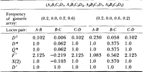
has the unfortunate property of being negative. An example of a situation in which these character- istics may be quite important is when using gametic frequencies to infer “recombinational hot spots” (e.g.,

CHAKRAVARTI et al. 1984). Let us assume that four loci or restriction sites, A , B , C and D , are tightly linked and that there is the maximum disequilibria present possible for the observed allelic frequencies. Two such gametic arrays are given in Table 12 with the calculated disequilibrium values. These arrays were chosen so that the frequencies of the alleles at loci A and B were equal and those at loci C and D were equal but different from A and B. For example, for the array given on the left, the frequency of A I and B , are 0.2 and that of CI and D I are 0.4. Notice that the disequilibrium values for all the measures except D’ are smaller between loci B and C than for locus pairs A-B and C-D. If one did not know that all the measures but D’ were dependent upon allelic frequencies, then it would appear that the disequili- bria between

B

and C was actually lower than for

A-

B and C-D. Such values have been used to suggest the presence of a recombinational hot spot which in this case may be only an artifact of the disequilibrium measure.

TABLE 12

Value of pairwise disequilibrium for the different measures for the frequency of four-locus gametes given in parentheses

Frequency

of gametic (0.2, 0.0, 0.2, 0.6) (0.2.0.0, 0.6, 0.2)

array:

1.orusnair: A-B B-C C-D A-B B-C C-D

D 2 0.102 0.006 0.102 0.230 0.058 0.102

D * 1 .O 0.062 1.0 1.0 0.375 1.0

1

.o

0.062 1.0 1.0 0.375 1.0

Q*

F’

X ( 2 ) 1.0 -0.103 1.0 1.0 0.370 1.0

D‘ 1

.o

1.0 1.0 1.0 1.0 1.0

2.125 -0.219 2.125 1.083 0.562 2.125

Another situation in which a frequency-dependent measure may lead to erroneous conclusions is in the examination of the effect of an evolutionary factor on disequilibrium. For example, FUERST and MARUYAMA

(1986) used

D *

to examine the effect of population bottlenecks on gametic disequilibrium and came to the conclusion that the extent of disequilibrium de- pended upon the allelic frequencies after the bottle- neck. However, the measure

D *

is itself a function of the allelic frequencies so it is probable that their conclusions are not due to the population bottleneck but to an artifact in the disequilibrium measure they

used.

Second, as stated in Table 11 the rate of decay due to recombination per generation in a large population is constant for D2,

D * ,

Q*

and D’ being the smallest. The rate of decay in this situation for F’ and X(2) varies over time and asymptotes at (1

-

c) or (1 - c ) ~ depending upon the initial gametic array.

Some general properties of the six measures are summarized in Table 13. For example, when samples from a population at equilibrium under neutrality are examined, in general F’ has the largest variance (and

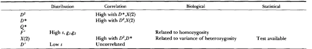
TABLE 13

Summary of general properties of the different gametic disequilibrium measures

Distribution Correlation Biological Statistical

D2 High withD*,X(2) D* High with Dz,X(2)

F’ High s, gJ&

D‘

Related to homozygosity

Q*

X(2) High with D2,D* Related to variance of heterozygosity Test available Low s Uncorrelated

frequency independent while all of the others have frequency dependence. Both F ’ and X ( 2 ) have some biological relevance (Table 13) while the other meas- ures have no particular relationship to biological en- tities such as homozygosity or heterozygosity. Addi- tionally, X ( 2 ) has a statistical advantage because of the presence of a statistical test (BROWN, FELDMAN and NEVO 1980).

From these considerations, in my opinion, one should proceed with caution when using a particular gametic disequilibrium measure. One should be care- ful to use a truly allelic frequency-independent mea- sure such as D’. The normalized measures D*, Q*,

F’ and X ( 2 ) are very frequency dependent. For ex-

ample, the good biological and statistical properties of

X ( 2 ) may be outweighed by its frequency-dependence,

negative values, and variable rate of decay. Further- more, the traditional propensity towards

D 2

and D

*

because of mathematical tractability may be less im- portant than their strong frequency dependence. As a result, prudence would suggest that D’ or some such frequency-independent measure of disequilibrium should be used to insure confidence in conclusions based on statistical associations of alleles at two (or more) loci.

I appreciate the comments of BILL HILL, BILL KLITZ, TOMOKO OHTA, GLENYS THOMSON and an anonymous reviewer on various aspects of this research. I also wish to thank BILL KLITZ and SING KAI-LO for their computer assistance. This research was supported by National lnstitutes of Health grants GM 35326 and HD 12731 to GLENYS THOMSON and University of California-Berkeley IBM ACIS.

LITERATURE CITED

AVERY, P. J. and W. G. HILL, 1979 Variance in quantitative traits due to linked dominant genes and variance in heterozygosity in small populations. Genetics 91: 817-844.

ASMUSSEN, M. A. and M. T. CLEGG, 1982 Rates of decay of linkage disequilibrium under two-locus models of selection. J. Math. Biol. 14: 37-70.

BISHOP, Y. M. M., S. E. FEINBERC and P. W . HOLLAND, 1975 Discrete Multivariate Analysis. MIT Press, Cambridge, Mass.

Multilocus structure of natural populations of Hordeum spontaneum. Ge- netic 96: 523-536.

CHAKRAVARTI, A., K. H. BUETOW, S. E. ANTONARAKIS, P. G. WABER, C. D. BOEHM and H. H. KAZAZIAN. 1984 Nonuniform recombination within the human &globin gene cluster. Am. J. Hum. Genet. 3 6 1239-1258.

BROWN, A. H. D., M. F. FELDMAN and E. NEVO, 1980

CLEGG, M. T., J. F. KIDWELL, M. G. KIDWELL and N. J. DANIEL, 1976 Dynamics of correlated genetic systems. I. Selection in the region of the Glued locus of Drosophila melanogaster. Ge- netics 83: 793-810.

EWENS, W. J., 1979 Mathematical Population Genetics. Springer- Verlag, Berlin.

FRANKLIN, I. R. and R. C . LEWONTIN, 1970 Is the gene the unit of selection? Genetics 65: 707-734.

FUERST, P. and T . MARUYAMA, 1986 Patterns of linkage disequi- librium generated by rapid changes in population size. Genetics

113: S44.

GOLDING, G. B., 1984 The sampling distribution of linkage dise- quilibrium. Genetics 1 0 8 257-274.

HEDRICK, P. W., 1980 Hitchhiking: a comparison of linkage and partial selfing. Genetics 94: 791-808.

HEDRICK, P. W., 1983 Genetics

of

Populations. Jones & Bartlett, Boston.

HEDRICK, P. W., S. JAIN and L. HOLDEN, 1978 Multilocus systems in evolution. Evol. Biol. 11: 101-182.

HEDRICK, P. W. and G. THOMSON, 1986 A two-locus neutrality test. Applications to humans, E. coli and lodgepole pine. Genetics

Linkage disequilibrium among multiple neu- tral alleles produced by mutation in finite population. Theor. Popul. Biol. 8 117-126.

Linkage disequilibrium in finite populations. Theor. Appl. Genet. 38: 226-231.

Properties of a neutral allele model with intragenic recombination. Theor. Popul. Biol. 23: 183-20 1.

T h e sampling distribution of linkage dise- quilibrium under an infinite-allele model without selection. Genetics 1 0 9 611-631.

KARLIN, S. and A. PIAZZA, 1981 Statistical methods for assessing linkage disequilibrium at the HLA-A, B, C loci. Ann. Hum. Genet. 45: 79-94.

LEWONTIN, R. C., 1964 T h e interaction of selection and linkage.

I. General considerations; heterotic models. Genetics 4 9 49- 67.

LEWONTIN, R. C. and K. KOJIMA, 1960 The evolutionary dynam- ics of complex polymorphisms. Evolution 14: 458-472. MARUYAMA, T., 1982 Stochastic integrals and their application to

population genetics, pp. 15 1-1 66. In: Molecular Evolution, Pro-

tein Polymorphism and the Neutral Theory, Edited by M. KIMURA.

Japan Scientific Societies Press, Tokyo.

Linkage disequilibrium between amino acids sites in immunoglobulin genes and other multigene families. Genet. Res. 3 6 181-197.

OHTA, T. and M. KIMURA, 1969 Linkage disequilibrium due to random genetic drift. Genet. Res. 13: 47-55.

SOKAL, R. R. and F. J. ROHLF, 1981 Biometry. W. H. Freeman, San Francisco.

SVED, J. A., 1968 The stability of linked systems of loci with a small population size. Genetics 59: 543-563.

YAMAZAKI, T., 1977 The effects of overdominance on linkage in a multilocus system. Genetics 8 6 227-236.

Communicating editor: M. T. CLEGC

112: 135-156. HILL, W. G., 1975

HILL, W. G. and A. ROBERTSON, 1968

HUDSON, R. R., 1983

HUDSON, R. R., 1985