Scholarship@Western
Scholarship@Western
Electronic Thesis and Dissertation Repository
12-11-2014 12:00 AM
A comparison of community composition analyses for the
A comparison of community composition analyses for the
assessment of responses to wood-ash soil amendment by
assessment of responses to wood-ash soil amendment by
free-living nematodes
living nematodes
Paul B.L. GeorgeThe University of Western Ontario Supervisor
Dr Zoe Lindo
The University of Western Ontario Graduate Program in Biology
A thesis submitted in partial fulfillment of the requirements for the degree in Master of Science © Paul B.L. George 2014
Follow this and additional works at: https://ir.lib.uwo.ca/etd
Part of the Other Ecology and Evolutionary Biology Commons, and the Terrestrial and Aquatic Ecology Commons
Recommended Citation Recommended Citation
George, Paul B.L., "A comparison of community composition analyses for the assessment of responses to wood-ash soil amendment by free-living nematodes" (2014). Electronic Thesis and Dissertation Repository. 2603.
https://ir.lib.uwo.ca/etd/2603
This Dissertation/Thesis is brought to you for free and open access by Scholarship@Western. It has been accepted for inclusion in Electronic Thesis and Dissertation Repository by an authorized administrator of
(Thesis format: Monograph)
by
Paul B.L. George
Graduate Program in Biology
A thesis submitted in partial fulfillment of the requirements for the degree of
Masters of Science
The School of Graduate and Postdoctoral Studies The University of Western Ontario
London, Ontario, Canada
ii
Abstract
Land-use changes can have far-reaching consequences for resident communities and
ecosystem functioning. Developing appropriate assessment methods to observe and quantify this change is an important application of community ecology. Here I compare four methods of community assessment for free-living soil nematodes under forest harvesting disturbance and wood ash application. Neither morphological assessment (richness, abundance, diversity) nor molecular assessment (morpho-richness using T-RFLP) was responsive to experimental treatments. Trait-based approaches (Maturity Index (MI) and Body Size Spectra (BSS)) were more sensitive to forest harvest and wood-ash amendment treatments. The efficacy of these methods was also qualitatively compared. Of all methods, the BSS were found to be the most informative and easiest to implement. Morphological assessment and the MI rely strongly on rare taxonomic expertise and T-RFLP requires considerable optimisation to be effective. The use of trait-based approaches for soil fauna is advocated as an accessible tool for community ecologists, especially those interested in taxonomically difficult groups.
Keywords
iii Co-Authorship Statement
iv
Acknowledgments
I must first give my heartfelt thanks Dr. Zoë Lindo for welcoming me into her lab. She has been patient, encouraging, and incredibly helpful. Such support allowed me to explore my interests during my time at UWO, and made this experience all the more special. This whole process has helped me build towards a future pursuing science that will both excite and challenge me. I could not have asked for a better supervisor.
I would also like to thank my advisors Dr. George Lazarovits and Dr. Greg Thorn. Their insights into the enigma of molecular processes were necessary to achieve my personal research goals. Dr. Thorn must be especially thanked for putting up with my frequent questions and allowing the use of his laboratory. Dr. Marc-André Lachance is also thanked for giving me a great introduction to molecular methods and whose assistance was invaluable in beginning this work. I also thank Dr. Melanie Columbus and Dr. Shawn Garner for the patience, teaching, and advice in this process. Dr. Ben Rubin’s comments on this thesis were necessary to bring it to its current quality.
My research was part of a collaborative effort between government agencies, the forestry industry, and community groups. Dr. Paul Hazlett was instrumental in allowing me to join the project. Thanks to Natural Resources Canada for the accommodation in Chapleau. Starting school mid-year, I was worried that it would be difficult to make friends having missed the previous semester. I could not have been more wrong. Matthew Turnbull, Danielle Griffith, and Catherine Dieleman welcomed me warmly to our lab. I hope to carry their friendships along with all those I made with my fellow graduate students, for a lifetime. I also have to thank the teammates and friends I have made as a member of the Western Mustangs rugby team and London St. George’s RFC. The camaraderie of the rugby
community is astounding, and in London this is certainly the case. My time here would not be the same without them.
Abstract ... ii!
Acknowledgments ... iv!
List of Tables ... vii!
List of Figures ... viii!
List of Maps ... ix!
List of Abbreviations ... x!
1! Introduction ... 1!
1.1! Effects of forestry practices on soil systems ... 1!
1.2! Nematode functional traits and the Maturity Index ... 4!
1.3! Body size as a response-effect functional trait ... 7!
1.4! Molecular markers of community composition ... 9!
1.5! Objectives ... 10!
1.6! Hypotheses & Predictions ... 10!
2! Methods ... 13!
2.1! Site description and experimental design ... 13!
2.2! Sampling regime ... 14!
2.3! Morphological analyses ... 15!
2.4! Trait-based analyses ... 16!
2.4.1! Maturity Index ... 16!
2.4.2! Body Size Spectra ... 17!
2.5! Molecular analyses ... 18!
2.6! Statistical analyses ... 19!
3! Results ... 23!
vi
3.2! Wood ash and the nematode community: trait-based measures ... 24!
3.2.1! Maturity Indices ... 24!
3.2.2! Body Size Spectra ... 25!
3.3! Wood ash and the nematode community: molecular assessment using T-RFLP . 26! 4! Discussion ... 35!
4.1! Response of the nematode community to clear-cutting ... 35!
4.1.1! Morphological measures of nematode communities ... 35!
4.1.2! Trait-based measures of nematode communities ... 37!
4.1.3! Molecular measures of nematode communities ... 38!
4.2! Response of the nematode community to wood ash amendment ... 39!
4.3! Evaluation of assessment methods by a priori criteria ... 41!
4.3.1! Evaluation of molecular T-RFLP assessment ... 41!
4.3.2! Evaluation of morphological community assessment ... 42!
4.3.3! Evaluation of trait-based community assessment ... 42!
4.4! Summary of results & recommendations ... 45!
References ... 48!
vii
List of Tables
Table 2.1: Results of nutrient analyses performed by the Canadian Forest Service – Sault Ste. Marie……… 21!
Table 3.1: Total abundance (per 25 g soil) of each taxon of free-living nematodes collected under forest, clear-cut and the three different wood ash applications from June 2013……... 27!
Table 3.2: Total abundance (per 25 g soil) of each taxon of free-living nematodes collected under forest, clear-cut and the three different wood ash applications from August 2013…... 28!
Table 3.3: Mean abundance, richness, diversity and evenness values by treatment from June and August samples………. 29 Table 3.4: Mean values of the trait-based indices, ΣMI, SI, and EI, as well as abundance by treatment from samples collected in June and August 2013 from the Island Lake Biomass and Harvesting Demonstration area near Chapleau, Ontario……….30
Table 3.5: Mean richness values of OTUs obtained from T-RFLP analyses in June and August sampling………..31 Table 4.1: Simplification of the results of qualitative assessment of each method of
Figure 1.1: A theoretical representation of the continuum of soil states determined by A) the Maturity Index (modified from Ferris et al. (2001) and B) their expected representation in a Local Size Density Relationship model BSS………... 12!
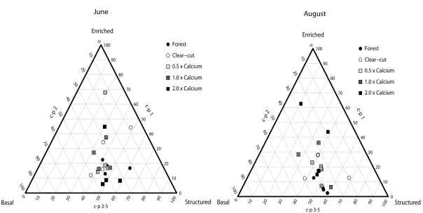
Figure 3.1: Weighted c-p triangles (ternary plots) showing the proportional distribution of c-p groups from each replicate of the forest, clear-cut, and ash-amended treatments in relation to the three soil states identified by the MI from June and August samples………32!
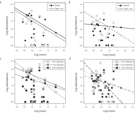
Figure 3.2: The nematode community as seen through the LSDR model of BSS using dry weight (ng) and abundance on a log10 scale of forest and clear-cut treatments in A) June and B) August, and one-half, equivalent, and twice Ca amendment in C) June and D) August.... 33!
Map 2.1: A map of the Island Lake Biomass Research and Demonstration Area, near
c-p: colonizer-persistor MI: Maturity Index
ΣMI: summed Maturity Index
EI: Enrichment Index SI: Structure Index BSS: Body Size Spectra
LSDR: Local Size Density Relationship ISD: Individual Size Density
H’: Shannon-Weiner’s diversity index J’: Pielou’s evenness index
1
Introduction
1.1
Effects of
forestry practi
ces on soil systems
Throughout history, human activities have altered natural systems to suit societal needs. Activities such as urban development, forest clearing, agriculture, and silviculture have altered nutrient and hydrologic cycling, increased global carbon dioxide emissions, degraded and fragmented habitats, and ultimately led to a loss in biodiversity (Foley et al., 2005). The effects of land-use change are well documented, particularly with regard to forest clearing and silviculture practices on soil systems (e.g. Huhta et al., 1967; Keenan & Kimmins, 1993) as well as their invertebrate communities (Huhta et al., 1967; Niemelä, 1997). In particular, communities of micro-invertebrates living within soils have been shown to respond to land-use change in agricultural land (e.g. Ou et al., 2005) as well as under various forestry regimes (Huhta et al., 1967; Panesar et al., 2000; Háněl, 2004).
Forest harvest methods in particular have varying effects on invertebrate communities. Nematode abundance, for example, was only marginally affected or unchanged following clear-cutting in Finnish forests (Huhta et al., 1967), whereas this disturbance caused a distinct decrease in nematode abundance in a Canadian temperate rain forest (Panesar et al., 2000). The causes of declines in soil invertebrates under
various forestry practices are often unclear as they occur in conjunction with other abiotic factors (i.e. site variability, climate, landscape changes). Further, responses to forest harvesting are not always consistent among groups of soil organisms, both taxonomic (Háněl, 2004) and trophic (Forge & Simard, 2001). For example, abundances of
nematodes have been shown to drop following clear-cutting (Huhta et al., 1967; Panesar et al., 2000), whereas this practice may increase the abundance other taxa like molluscs and Collembola (Marshall, 2000).
2014), with frequent fire (Bergeron et al., 2002a) and cyclic outbreaks of insect pathogens (Volney & Fleming, 2000) as the prominent drivers of tree species
composition. Harvesting within the Boreal zone has a lengthy history across the country (Volney & Fleming, 2000) and has generally consisted of clear-cutting followed by short-rotation, even-aged plantations (Bose et al., 2014). However, forestry practices have lately become more focused on ecosystem management practices (Attiwill, 1994; Bergeron et al., 2002b) as it is thought that these approaches will help support endemic species and increase ecosystem resilience (Drever et al., 2006). Ecosystem management practices can be broadly grouped together as partial or selective cutting methods
including shelterwood harvesting (leaving remnant patches), commercial thinning (strip cutting), and diameter-limit cutting (minimum size) amongst others (Bose et al., 2014).
Forestry interests are also looking to increase their annual timber yield whilst simultaneously implementing better management practices. Previous use of clear-cutting has in many cases resulted in the removal of nutrients including: carbon (C) (Grand & Lavkulich, 2012), nitrogen (N), phosphorous (P), potassium (K), and calcium (Ca) (Hornbeck & Kropelin, 1982). This has led to research for possible amendments to reintroduce these nutrients or mitigate the effects of their removal. Wood ash has been identified as one such amendment and has been applied successfully in both agriculture and silviculture (Augusto et al., 2008). Indeed, since as early as 1935, wood ash has been applied to forest soils in attempts to restore biodiversity in acidified soils (Pitman, 2006). Wood ash amendment used in silviculture is generally produced through the combustion of coniferous and deciduous stems, slash, or refuse generated in paper production. The use of wood ash amendment is common across Scandinavia and is growing in popularity in some parts of the United States (Pitman, 2006). However, despite its substantial use in Canadian agriculture (Arshad et al., 2012; Jaramillo-Lopéz & Powell, 2013) wood ash has rarely been applied in Canadian forests (see McDonald et al., 1994).
typically has a greater concentration of Ca for example (Pitman, 2006). The most
beneficial effects of wood ash amendment are an increased ability to retain soil moisture (Pitman, 2006) and increase pH (Arshad et al., 2012). These effects stem from the high neutralising capacity of ash (Deymeyer et al., 2001) and the subsequent increase in dissolved organic C post-amendment. Vance (1996) proposed that wood ash could fill the role of commercial NPK fertilisers, despite containing lower percentages of these
nutrients than traditional products (Naylor & Schmidt, 1989). However, the fertilising effect of ash is likely negligible or minor at best as the majority of both P and K are immobilised in ash (Pitman, 2006) and N is not present in ash (Augusto et al., 2008). However, it should be noted that amendment can increase N availability indirectly through an increase in pH (Vance, 1996).
Wood ash may also have harmful effects on the soil as it can contain substances such as heavy metals and polyaromatic hydrocarbons (Pitman, 2006; Augusto et al., 2008). Wood ash application has been linked to changes in plant (Pitman, 2006; Augusto et al., 2008), microorganism (Pitman, 2006), and animal communities (Nieminen, 2011). However, these changes vary in their magnitude, potentially due to abiotic factors
stemming from soil-wood ash interactions (Pitman, 2006). For example the meta-analysis of Augusto et al. (2008) found wood ash had no effect on tree growth in mineral soils but that growth was positively affected in organic soils. Herbaceous plants (Pitman, 2006) and grasses (Arvidsson et al., 2002) also respond positively to amendment whereas bryophytes (Kellner & Weibull, 1998), shrubs, and lichens (Jacobson & Gustafsson, 2001) commonly respond negatively. Soil fungi have also been shown to display positive (Pitman, 2006) and negative (Nieminen & Setälä, 2001) responses.
Studies quantifying the response of the nematode communities are generally indirect as they are commonly quantified in conjunction with the enchytraeid community and/or used as indicators of microorganism responses (Nieminen & Setälä, 2001; Lirri et al., 2007). In these cases it was determined that nematode abundances were altered indirectly via changes in food sources; Lirri et al. (2007) found that the biomass of ectomycorrhizal fungi was reduced in wood ash amended mesocosms compared to controls, with a
corresponding reduction in the number of fungivorous nematodes. This result is similar to those of Nieminen and Setälä (2001) although they suggested that nematode feeding preference may have influenced the results. It should also be noted that both of these experiments took place in ex situ mesoscosms, whose fidelity to the natural state can be limited by factors like extreme nutrient limitations, loss of natural functions (Nieminen, 2011), and loss of uncommon species (Verhoef, 1996). Bååth et al. (1995) suggest that bacterivorous nematodes are more likely to increase in abundance than fungivores following wood ash amendment as fungi appear to be generally less tolerant of ash amendment. This suggestion has been supported in mesoscosm experiments that found limed soils support greater bacterial abundances than unlimed controls and thereby a larger bacterivorous nematode community (Räty & Huhta, 2003). Wood ash amendment in forest soils in situ has shown that total nematode abundance initially increased with a brief spike in fungivores immediately after amendment, while the proportion of
bacterivores is sustained (Lirri et al., 2002). However, Huhta et al. (1983) found that populations of all soil invertebrates declined after three weeks of exposure to wood ash in a mesocosm study, despite an initial increase in nematode abundance. The effects of wood ash amendment on other nematode feeding groups, including predators, remain unclear.
ease of sampling (Ferris et al., 2001). However, nematode taxonomic expertise is becoming increasingly rare and has a steep learning curve (Chen et al., 2010). This makes quantifying nematode diversity and interpreting community changes and their consequences difficult.
The study of functional traits has become popular in modern ecological theory. Functional traits are life history characteristics of organisms can alter an ecosystem’s functions (effect traits) or respond to environmental changes (response traits), in
particular, anthropogenic disturbance (Suding et al., 2008). The study of functional traits has been instrumental in allowing researchers to investigate both how organisms
influence and respond to changes in the environment. Functional traits influence an individual’s growth, reproductive ability, and survival imparting an overall effect on its fitness (Violle et al., 2007). They have received much more attention in plants than animals (Violle et al., 2007; Suding et al., 2008), and even less so in soil invertebrates. There has been little exploration of effect traits in animals; however, studies focused on response traits such as body size are more common in the literature (e.g. Mulder & Elser, 2009).
stability and thus ‘maturity’ through succession. The majority of nematode species have traits that fall within the r/K continuum, and are classified as c-p levels 2 through 4. Body size has also been shown to generally correlate with the progression of the c-p scale with an increase in body size following the r/K-selection continuum (Vonk et al., 2013).
Using the c-p scale is advantageous as it incorporates both response traits (e.g. body size), which predict how a taxon will react to disturbance, and effect traits (e.g. trophic level) that influence processes including decomposition (Adl, 2003) and trophic transfer efficiency (Lindo et al., 2012). The c-p groups are also related to feeding preferences (Bongers & Bongers, 1998), which are also typically related to body size. Generally, nematodes can be assigned directly to c-p groups at the family-level but lower units (i.e. genus) may be different enough from related taxa to warrant membership to a different c-p group. Many authors who use the MI will include the c-p rankings of
families and genera that they study (e.g. Bongers, 1990; Bongers & Bongers, 1998; Ferris & Matute, 2003; Mills & Adl, 2011), which is helpful, but the c-p designation of
undescribed or previously unassigned species, is still required (Bongers, 1999). The MI is calculated as follows:
(1)
!" = !(!)⋅!(!) !
!!!
where f(i) represents the frequency of taxon i (of n taxa) in a sample and v(i) is the c-p value of taxon i (Bongers, 1990). The MI uses the relative proportions of different functional groups within the nematode community to classify a soil as: basal, enriched, or structured (Bongers & Bongers, 1998; Ferris et al., 2001). Structured soils are
dominated almost exclusively by generalist bacterivores (c-p 1). Over time, soils will become increasingly structured from either the basal or enriched state, as niche space will slowly open up for c-p 3 through c-p 5 taxa, which add trophic links to the community and increase its diversity (Ferris et al., 2001). The MI has produced many derivatives over the past 25 years. When it was originally created, the plant-feeding nematodes of the community were excluded from the calculation (Bongers, 1990), but Yeates (1994) has included this trophic group in the MI by utilising their c-p values and abundances (denoted as the ΣMI with the inclusion of plant-feeding nematodes). Additional indices developed by Ferris et al. (2001) have allowed the community to be further explored by representing the expected responsiveness of the dominant feeding-groups of structured and enriched soils (the SI and EI, respectively). Such derivatives allow for finer-scale details of a community’s composition to be understood.
1.3
Body s
ize as a response-
effect functional trait
As mentioned previously, with some exceptions, body size increases with c-p level (Vonk et al., 2013) making it a component of MI values. Recently, Turnbull et al. (2014)
postulated that body size might be used independently as a response trait metric in free-living soil nematodes. This notion works on the framework that during community disassembly, species loss is determined by the presence or absence of traits (Zavaleta et al., 2009), and that larger species are more likely to go extinct after habitat disturbance (Leck, 1979; Gonzalez & Chaneton, 2002; Cardillo, 2003). Furthermore, studies of soil community responses to disturbance have shown body size as a predictor of extinction risk, and therefore a response to environmental change (Mulder et al., 2008; Mulder & Elser, 2009), as well as trophic interactions and resource utilisation (Mulder et al., 2009; Mulder et al., 2011). Community wide body size measures can be shown for any given system by using abundance-by-body size plots called body size spectra (BSS) to observe community-level responses to disturbance. Indeed, the use of BSS is common in
assessing the effects of disturbance in aquatic systems (Sprules & Munawar, 1986; Transpurger & Bergtold, 2006; White et al., 2007; Petchey & Belgrano, 2010), whilst several studies have also shown the value of BSS in studying soil invertebrate
White et al. (2007) review two methods of assessing BSS, both of which can be applied to soil communities. The first is the local size-density relationship (LSDR) model, in which a species’ average body size is plotted against its population density (Turnbull et al., 2014) on a log-log scale. The second model works without species identification and is known as the individual size distribution (ISD) model. This method groups body size values into classes and plots them against the log population densities of individuals per size class (Turnbull et al., 2014). Both methods have been applied in soil systems (Mulder & Elser, 2009; Lindo et al., 2012).
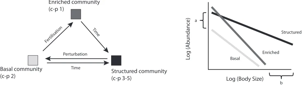
The use of BSS to visualise changes in nematode and other soil invertebrate communities following disturbance, and as a community-wide metric of change or perturbation was recently proposed by Turnbull et al. (2014). Here, they demonstrate how a BSS approach could be used to demonstrate the changes in nematode communities observed using the MI. As body size generally scales with c-p level (Ferris et al., 2001), it is expected that an overall reduction of large-bodied species would be observed under disturbance in a basal MI community, and an overall increase in the abundance of small-bodies species following nutrient addition in an enriched MI community. Visually this would manifest in the BSS plot as differences in intercept and slope of the regression from the log-abundance by log-body size plot (LSDR model), where the structured MI BSS would have a shallow negative slope, the basal MI community would demonstrate a steepening in slope, and the enriched MI community would have a steepened slope and higher intercept (Figure 1).
The slope of the LSDR BSS model, whilst indicating change in the relative abundance of body sizes following non-random species loss (i.e. body size as a response trait), has also been proposed to reflect the trophic transfer efficiency (TTE) of a
been useful and corroborated in aquatic and marine systems, but has not yet been examined for terrestrial systems.
1.4
Molecular markers of community composition
Currently, many biological researchers feel that the use of unique DNA markers is needed to gain a better understanding of biodiversity. Indeed, there has been a popular push to compile unique gene sequence to form the Barcode of Life (Herbert & Gregory, 2005), and a number of other molecular-based methods for community analysis have also been developed. These approaches have allowed researchers to identify quickly and accurately the constituents of communities that can be difficult to ascertain via traditional taxonomic means (Donn et al., 2008). This is especially true of cryptic species (Trewick, 2000) as well as microorganisms (Moreira & López-García, 2002). This method often relies on use of the cytochrome c oxidase 1 gene, which is underreported in nematodes with researchers favouring use of the 18S rRNA gene (Chen et al., 2010). There is also a strong push towards the use of next generation sequencing techniques for community analyses (Taylor & Harris, 2012). Yet, for nematology, next generation sequencing is still in early development (Chen et al., 2010; Martin et al., 2012).The T-RFLP method has been applied successfully to nematode communities in agricultural, dune, forest, and wetland soils (Donn et al., 2008; Donn et al., 2012). However, despite their popularity, molecular methods can prove challenging for beginners, difficult to troubleshoot (Maurer, 2011), and in some cases not ideal for identifying certain taxa (e.g. Cephalopoda, see Strugnell & Lindgren, 2007). Prakash et al. (2014) describe a number of potential areas of concern specifically for T-RFLP analyses including biased cell lysis, incomplete enzyme digestion, and variation in sample size. These problems can become especially apparent when molecular methods are applied to a new system. A full comparison of morphological, trait-based and molecular-based approaches to understand a change in nematode communities under disturbance has not been performed.
1.5
Objectives
This study had three objectives. (1) quantify the effects of wood ash amendment on nematode abundance and diversity. This was done by identifying and enumerating nematodes at the finest level of taxonomic resolution possible and utilising the Shannon-Weiner Index and the MI to detect differences in taxonomic and functional diversity. (2) use BSS to evaluate changes in nematode community structure in response to forest harvest disturbance and subsequent amendment as a trait-based approach. This was determined by comparing the responses of the community via changes in the c-p groups for the MI, and changes in body size using LSDR and ISD models of BSS. (3) quantify changes in diversity and community structure using the molecular T-RFLP approach. These objectives all come together under the goals of assessing the overall impacts of wood ash amendment on free-living nematodes whilst also comparing the efficacy of the four methods (morphotaxa identifications, MI and BSS functional traits, and T-RFLP analysis) used to quantify diversity in the study.
1.6
Hypotheses & Predictions
enrich the soil, resulting in an increased proportion of c-p 1 nematodes, further altering the MI values, which would be amplified with increasing wood ash load. For the BSS, I predict that in the LSDR model a lowered intercept under forest harvesting and a steeper slope and increased intercept to be seen under wood ash application. In the ISD model, I expect that there will be a reduction in the abundances of larger size classes following harvest and an increase in smaller classes under wood ash application. Lastly, I predict that T-RFLP analyses will show similar trends in the reduction of morpho-richness to the morphological assessments. Since comparisons between these methods cannot be
empirically calculated, each method’s effectiveness was qualitatively assessed based on the three following a priori criteria. (1) Is the method informative? In this case, an informative metric will provide information on the community’s sensitivity to treatment effects and give some insight into the mechanisms behind them. (2) Is the method
Figure 1.1: A theoretical representation of the continuum of soil states determined by A) the Maturity Index (modified from Ferris et al. (2001) and B) their expected representation in a Local Size Density Relationship model BSS. A) Basal nematode community is dominated by c-p 2 taxa, generally small-bodied fungivores and bacterivores in a recently disturbed food-web. With fertilization, the proportion of c-p1 taxa (exclusively bacterivores) increases following an influx of resources post-disturbance to create an Enriched community. Both of these states will mature into Structured communities given time without disturbance and increased resource availability, where larger-bodied and greater diversity of trophic groups exist. Under B) initial Structured communities have a shallow BSS slope; following perturbation, as the community shifts to the Basal state, we observe loss in overall abundance (a) and a
disproportionate loss in large-bodied species (b). This results in an overall steepening of slope. Following post-disturbance
fertilisation, the increase in small-bodied species increases overall abundance (Enriched), but the BSS slope remains steep compared to that of the Structured community. Figure reproduced with permission from Turnbull et al. (2014).
phytoplankton to large consumers and found that TTE reduced as body size increased and did not change with alterations in net primary production.
There are also examples of the application of BSS on studies of soil communities. Energy equivalence, for instance, has been demonstrated in arthropods extracted from forest soils (Kampichler, 1995; Meehan et al., 2006), where both studies found that small-bodied arthropods use the same amount of energy
within each size class observed.Kampichler (1995)theorised that
this may be due to larger size classes having the ability to consume a larger volume of food per unit time, whereas smaller size classes may more effectively perceive their environment at small scales allowing them to access resources that larger size classes cannot
obtain.Mulder and Elser (2009)also described changes in soil
or-ganism BSS and food web structure in response to changes in C:N:P ratios and acidity, and found increasing available P alleviated food constraints on smaller primary consumers (microbiovores) thereby allowing larger consumers at higher trophic positions to increase in
abundance. This was supported byMulder et al. (2009)in a study of
Dutch meadows and heathlands, where again higher P availability was related to shallower BSS slopes indicating a more even body size distribution. Collectively, these works support a shallow BSS slope indicating increased TTE.
However, the application of BSS to TTE and energy equivalence is not always a simple process. Indeed, most conclusions about TTE
were drawn from aquatic studies using ISDs (e.g. Jennings et al.,
2002; Blanchard et al., 2009), instead of the LSDRs that are more
fitting for soil ecologists. However, we expect LSDR models to more
accurately describe these relationships and illuminate exceptional cases because the abundance of each species is more easily visual-ized. Studies of TTE in aquatic systems also rely on stable isotope
analysis (Jennings et al., 2002; Jennings and Mackinson, 2003), a
process that is currently being applied to soil systems to infer
tro-phic position (Scheu and Falca, 2000; Schmidt et al., 2004; Crotty
et al., 2011). Yet stable isotope analyses can be problematic for soil
fauna due to their small size and complex feeding strategies (Scheu,
2002). Further, the sheer complexity and overlapping nature of soil
food webs presents problems with establishing definitive trophic
placements (Crotty et al., 2012).Mulder et al. (2009)used enzymatic
information for defining feeding groups to overlay soil food web
characteristics on the BSS following a calculation from aquatic
sys-tems byReuman and Cohen (2004). Here, trophic link length was
calculated as the difference in body size and abundance of con-sumers and their resources. While this demonstrates that body size can be linked to food webs, further work is needed to gain direct, independent measures of TTE. Similarly, the expected outcome of
the energy equivalence rule proposed byDamuth (1981)does not
precisely match the results ofKampichler (1995)andMeehan et al.
(2006), possibly due to inherent differences between endothermic
mammals used in Damuth’s study, and ectothermic invertebrates in
soil systems (Gillooly et al., 2001). It has been theorized that global
size density relationships break down at the local scale (Blackburn
and Gaston, 1997; White et al., 2007; but seeCyr et al., 1997), but this has not been extensively explored in soil systems.
5. Caveats, challenges and limitations
Assessment of BSS involves simple modelling and image capture software, making it an easily accessible option for individuals interested in community change but lacking the time needed for in depth taxonomic training. It can be used in conjunction with more
traditional studies (e.g. the nematode Maturity Index) to confirm
the results of functional diversity measures. We propose that with the popularity of functional diversity assessments and the relative ease of BSS construction, incorporating body size as a community metric can enhance the pertinence of many soil ecology studies. Aquatic ecologists have long recognized the applicability of the BSS to taxonomically diverse systems with complex trophic in-teractions to generate functional conclusions and reveal emergent
size-based relationships (Jennings et al., 2001, 2002; Cohen et al.,
2003). Similarly, the BSS is expected to serve well in exceptionally
diverse soil communities where the vast majority of species are
undescribed (Wall et al., 2005), but this is not without challenges.
The extent to which the taxonomic, developmental and func-tional group differences between and among organisms will modify basic allometric relationships is still an area of consider-ation. While we expect allometric relationships to hold true both within and across taxa, known and observed deviations due to
these factors strongly suggest that species identification will
remain a crucial component of body size analyses (Petchey and
Belgrano, 2010). For example, Blanchard et al. (2009) found
significantly steeper BSS slopes in predatory marine fauna
compared to detritivorous communities, indicating trophic roles
can modify the body size eabundance relationship. This has not
Fig. 1. Comparison of theoretical nematode communities as visualised underA)nematode ColoniserePersister Scale of the Maturity Index, modified fromFerris et al. (2001), andB) hypothetical Body Size Spectra based on the relationship of nematode abundance and body size. UnderA)a Basal nematode community is indicated by the dominance of cep 2 taxa egenerally small-bodied fungivores and bacterivoresein a recently disturbed food-web. With fertilisation the proportion of cep 1 taxa (almost exclusively small-bodied bac-terivores) increases following an influx of resources post-disturbance to create an Enriched community. Both of these states have the potential to develop into Structured com-munities given greater time without disturbance and increased available resources, where larger-bodied and greater diversity of trophic groups exist. UnderB)initial Structured communities have a shallow BSS slope; following perturbation, as the community shifts to the Basal state, we observe loss in overall abundance (a) as well as a disproportionate loss in large-bodied species (b). This results in an overall steepening of the slope of the BSS. Following post-disturbance fertilisation, the increase in small-bodied species increases overall abundance (Enriched), but the BSS slope remains steep compared to that of the Structured community.
M.S. Turnbull et al. / Soil Biology & Biochemistry 68 (2014) 366e372
2
Methods
2.1
Site description and experimental design
Sampling took place at the Island Lake Biomass Harvest Research and Demonstration area located in the Martel Forest near Chapleau, Ontario (47°50’N, 83°24’W). This site was developed through collaboration between forestry companies (Tembec,
FPInnovations), provincial (Ontario Ministry of Natural Resources) and federal
(Canadian Forestry Service) governments, as well as First Nations (Northeast Superior Chief’s Forum) and other community supporters (Northeast Superior Forest Community).
Consisting of sandy, glaciofluvial soil, the area was previously a jack pine (Pinus
banksiana Lamb.) plantation, which was harvested in 1959. Currently, both jack pine and
black spruce (Picea mariana (Mill.) Britton, Sterns & Poggenb.) are being replanted as
part of other ongoing experiments. Forest plots were covered in moss carpets and supported a population of approximately 40-year-old jack pine. Clear-cut and ash amended plots were sparsely covered in vegetation in June but vegetation cover was noticeably greater in August. In these plots grasses, small forbs, and shrubs, especially
blueberry (Vaccinium sp.), were the most common plants.
The experiment had a randomised block design (Map 2.1). Replicate plots were established within a 41.5 ha area that was clear-cut in winter 2011, followed by site preparation (summer 2011) and hand ash application in fall 2011. Ash was generated from branches, bark and other slash collected during harvesting in Tembec’s
Kapuskasing cogeneration plant using air scrubbers and collection trays below the grates to collect the ash. Wood ash produced at this site contains ~ 20% Calcium (Ca) (for
further explanation see Kwiaton et al., 2014). Three ash treatments were applied to each
of four replicate 25 x 25 m plots equating to the addition of: 1) one-half of Ca removed through harvest (100 kg/ha) 2) equivalent Ca (200 kg/ha), and 3) twice the Ca removed through the harvest of full-tree biomass (400 kg/ha). The ash treatment plots were
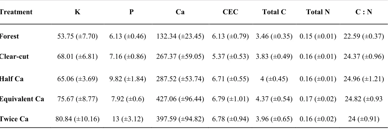
A preliminary assessment of soils was performed in June 2013. Few differences in variables were found and are therefore summarised here as site information only (Table 2.1). Soil pH ranged from 5.04 - 5.22 with no significant difference among treatment plots, but was lowest in clear-cut plots and highest in twice Ca amended plots. Soil moisture content was determined for each plot using the formula:
(2)
!"#$%&'(!!"#$%#$= !"−!"
!" ∙100%
where FW is the fresh weight of soil samples before drying and DW is the dry weight of the soil after it has reached a constant weight (i.e. all moisture has evaporated) following 24 hours of drying at 60°C. Soil moisture ranged from 41.15% in the forest plots to 44.67% in the twice Ca amended plots; no significant soil moisture conditions were observed among treatments. The organic layer of the soil across the harvested plots was
quite thin (35.46 ± 1.28 mm); however, it was significantly deeper in forest plots (55.30 ± 6.18 mm). Acute toxicity of wood ash was tested for using an International Standard Operation with the Collembola species Folsomia candida (Environment Canada, 2007). There was no evidence of toxicity. Nutrient analyses provided by the Canadian Forest Service did not show significant differences in K, total C, total N, exchangeable P, cation exchange capacity, or C : N ratio. Interestingly, there were no significant differences in Ca between treatments; however, soil Ca content did follow the expected trend of being lowest in forest plots and highest in twice Ca amended plots.
2.2
Sampling regime
Sampling occurred in June and August 2013. At each plot, eight subsamples of
Western Ontario for nematode extraction within 72 hours. Upon arrival at Western, soil samples were kept at 4 °C until extractions and assays were run.
Nematodes for morphological and molecular analyses were extracted from soil cores using the Baermann funnel technique (Forge & Kimpinski, 2008). For
morphological analyses, nematodes were extracted and fixed in 4% formalin solution, stained with Rose Bengal, and mounted with Permount® prior to microscopic
observation for body size measurements, identification, and enumeration under 400X magnification. This process involved taking a fixed and stained sample and pouring it into a watch glass under a dissecting microscope at 5x magnification. As nematodes were observed they were collected using a 10 µL pipette to move them in large numbers from the sample liquid to the Permount medium on a microscope slide. Ten to 20 specimens were mounted per slide. For molecular analyses, nematodes were extracted from separate aliquots into water, centrifuged, and stored at -20 °C until DNA extraction and the
terminal restriction fragment length polymorphism (T-RFLP) process.
2.3
Morphological analyses
Slides were scanned visually with a compound microscope at magnifications of 100-400X. When a nematode was observed it was identified to morphotaxa (i.e.
morophologically distinguishable species types) at the genus and family level based on keys from Bongers (1994) and the University of Nebraska – Lincoln (Tarjan et al., 1977) under 100-400X magnification. The taxonomic richness of each 25 g wet soil weight sample was estimated by summing the number of morphotaxa in each sample. Similarly, the abundance of each morphotaxon was estimated by enumerating the total number of individuals from each morphotaxon in every 25 g wet soil weight sample. These data were used to calculate Shannon-Weiner’s diversity index (H’) for each sample through the equation:
(3)
!! =!−Σ !
where pi is the relative proportion of each morphotaxon’s abundance in terms of total abundance (Shannon, 1948). This value was subsequently used to find Pielou’s evenness for each sample using the formula:
(4)
!! =! !′ ln !
where S is the number of morphotaxa in the community (Pielou, 1975). Community composition of the samples also was assessed using morphotaxa identities, richness and abundance of each species. For these indices, unknown individuals were dropped from the analyses.
2.4
Trait
-
based analyses
2.4.1 Maturity Index
Nematode families and genera were assigned to the c-p scale following their
identification as prescribed by Bongers and Bongers (1998). These values were then used to calculate the ΣMI as described by Yeates (1994). This metric uses the equation of the original MI (Bongers, 1990) (Equation 1). However, the MI as described by Bongers (1990) excludes plant-feeding nematodes. Yeates’ ΣMI is different in that plant-feeding nematodes and their c-p values are permitted in the equation (1994). The ΣMI was further broken down into the structure index (SI) and enrichment index (EI). These values are presented as percentages and reflect the position of the community along the gradient of soil conditions posited by the MI (Ferris et al., 2001). These were calculated using the formulae from Ferris et al. (2001):
(5)
!" =100%∙( !
(6)
!"= 100%∙ !
!+!
These calculations incorporate the importance of feeding groups of bacterivore,
fungivore, omnivore, plant-feeder, and predator into the c-p scale. Groups that are more indicative of a structured or enriched community receive higher weights than basal groups. For this study the weights of each feeding group were derived from Ferris et al. (2001). In both cases b denotes the basal component of the community calculated as the sum of the basally weighted taxa using the formula:
(7)
!=! !"∙!"
where, k is the weight assigned to the basal feeding groups assigned by Ferris et al. (2001) and n is the total number of individuals in that each basal group. Similar equations for s and e are used (i.e. instead of b), which utilise the weights (k) associated with structure and enrichment (Ferris et al., 2001).
2.4.2 Body Size Spectra
Following morphological identification, the length and width of each nematode were measured on slide-mounted specimens. For June samples, this was done by digitally capturing the nematode specimen as an image and making calibrated measurements of body length and width using ImageJ® software. For August samples, length and width measurements were made through a digital camera mounted on the microscope and the automated image analysis software program NIS - Elements that can measure calibrated lengths of objects (Nikon Corporation, 2013). This digital imaging system reduced processing times for body size measurements to about 20% of those measured in June.
(8)
!"#!!"#$ℎ!!(!") =( 530∙!∙!! ×1.084) 4
where L is the total length (mm) and W width (mm). This volume is then converted to wet weight (µg) using the specific gravity of 1.084 (Weiser, 1960) and then to dry weight (µg) assuming a dry/wet weight ratio of 0.25 (Juario, 1975). Dry weights were used as body size in two types of BSS. First a Local Size Density Relationship (LSDR) model was created. This model is a regression between the log10 average abundance of each species and the log10 value for the average body size of that species. In this case, average taxon-specific dry weight was determined from 10 randomly selected individuals (or as many as possible when abundances were less than 10). These data were visualised using a scatter plot with regression lines that were determined in the 75th quartile using the package “quantreg” (Koenker, 2005) in R version 2.14.1 (R Development Core Team, 2014). This method was use to reduce the influence of rare taxa.
The other type of BSS used is the Individual Size Distribution (ISD) model sensu
White et al. (2007). This method uses individual body sizes (x) (without species
identities) binned into log2 (x + 0.5) size classes plotted by the average abundance of each class. This method was used to observe purely qualitative trends and as a result, no
statistical analyses were conducted.
2.5
Molecular analyses
The process of extracting DNA for T-RFLP analysis began with breaking up individual nematodes using bead-beating in conjunction with PureLink® genomic DNA extraction kits. This was followed by further purification using a Zymo DNA clean and concentrator kit® and then PCR using the forward primer Nem_SSU_F74 (5’
AARCYGCGWAHRGCTCRKTA 3’) with the fluorescent label 6-fluorescein amidite (6-FAM), the reverse primer SSU_R_81 (5’ TGATCCWKCYGCAGGTTCAC 3’) (Donn
forward primer, 1.25 µL reverse primer (both at 20 pMolar concentration), and 5 µL DNA template. A positive control for the PCR was derived from a commercial culture of the nematodes Heterorhabditis bacteriophora and Steinernema carpocapsae. The PCR reaction was conducted in a thermocycler following the method of Donn et al. (2011): 94 °C, 2 min; then 35 cycles of 94°C, 30s; 51 °C, 1 min; 68 °C, 2 min and a final extension step of 68 °C for 10 min. This process yielded a product of approximately 1750 base pairs that was subsequently digested with HinfI restriction endonuclease (Donn et al., 2012) in a 32 µL reaction consisting of: 10 µL PCR reaction mixture, 18 µL nuclease-free water, 2 µL 10X buffer R, and 2 µL Hinf1. The digestion products were sent to the
Advanced Analysis Centre at the University of Guelph where they were processed using a 500 LIZ size standard and returned for statistical analyses.
Restriction fragment analyses were conducted using GeneMarker (Softgenetics), which produces an output that displays bands as peaks. This allowed for the
quantification of the number of operational taxonomic units (OTU) (i.e. peaks) into a richness value for each 25 g wet soil weight sample. These data were used to conduct community comparisons as described below.
2.6
Statistical analyses
In the LSDR model, the slopes and intercepts of the body size spectra for each treatment were calculated using 75% quantile regression and compared using analysis of covariance (ANCOVA). The ISD model of body size spectra was assessed visually without further statistical analyses. Body size spectra were analysed (or visualized for the ISD model) separately for June and August samples. The richness and relative abundance of OTU’s based on the molecular assessment of the nematode communities (T-RFLPs) were compared using RM-ANOVA followed by Tukey post hoc testing where
Table 2.1: Results of nutrient analyses performed by the Canadian Forest Service – Sault Ste. Marie. Mean values are expressed as ppm for K, exchangeable P, and Ca, as me/100g for CEC, as percentage for total C and N, and as a ratio for C : N. Standard errors are listed in parenthesis.
Treatment K P Ca CEC Total C Total N C : N
Forest 53.75 (±7.70) 6.13 (±0.46) 132.34 (±23.45) 6.13 (±0.79) 3.46 (±0.35) 0.15 (±0.01) 22.59 (±0.37)
Clear-cut 68.01 (±6.81) 7.16 (±0.86) 267.37 (±59.05) 5.37 (±0.53) 3.83 (±0.49) 0.16 (±0.01) 24.37 (±0.96)
Half Ca 65.06 (±3.69) 9.82 (±1.84) 287.52 (±53.74) 6.71 (±0.55) 4 (±0.45) 0.16 (±0.01) 24.96 (±1.21)
Equivalent Ca 75.67 (±8.77) 7.92 (±0.6) 427.06 (±96.44) 6.79 (±1.01) 4.37 (±0.54) 0.17 (±0.02) 24.82 (±0.93
3
Results
3.1
Wood ash and the nematode community:
morphological assessment
Samples collected in June and August 2013 yielded a total of 5377 nematode individuals that could be identified into a total of 26 morphotaxa. In June samples, 3437 individual nematodes were enumerated of which, 2933 were identified using morphological characteristics from Tarjan et al. (1977) and Bongers (1994). These individuals were classified to 20 genera and 2 families that could not be further subdivided for a total of 22 morphotaxa (Table 3.1). The most abundant groups at this time were: Plectus sp.,
Acrobeloides sp., and Rhabditidae sp. August sampling yielded a total of 1940
nematodes, of which, 1741 were identified to 22 genera and 2 families from which no further identifications could be made (24 total morphotaxa) (Table 3.2). The most
common taxa in the August samples were: Acrobeloides sp., Plectus sp., and Rhabditidae sp.
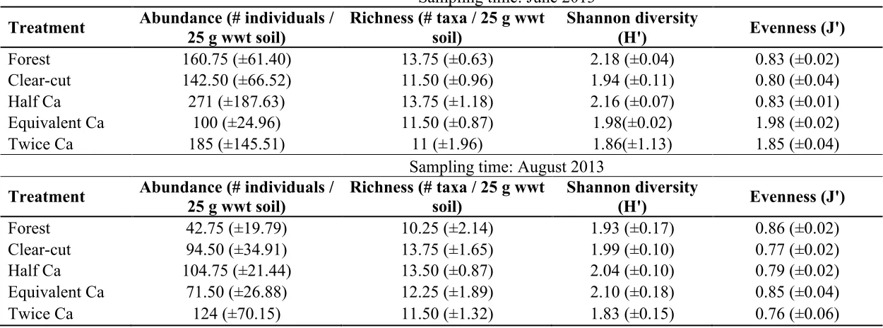
The RM-ANOVA for morphotaxa richness did not suggest any differences among treatments (F4, 15 = 0.675, p = 0.620), sampling time (June versus August) (F1, 15 = 0.004,
p = 0.953), nor a time by treatment interaction (F4, 15 = 1.309, p = 0.311). In June, the
forest and one-half treatments were equally the most species rich, supporting on average 13.75 species per 25 g wet weight soil, whereas the twice Ca plots were the lowest (11.00 species / 25 g wwt soil). August samples showed a much different trend, with clear-cut plots hosting an average of 13.75 species but only a mean of 10.25 species / g wwt soil were present in the forest treatment.
Overall sampling densities ranged between 400 individuals/25 g wet soil in the equivalent Ca plots and 1084 individuals/25 g wet soil in the one-half Ca plots in June, and 190 individuals/25 g wet soil in the forest plots to 552 individuals/25 g wet soil in the twice Ca plots in August (Table 3.3). However, repeated measures ANOVA found no significant differences in mean abundance between the five treatments (F4, 15 = 0.335, p =
0.384, p = 0.817). Mean values of H’ (Shannon diversity) were highest in the forest treatment and reached their low point in the twice Ca amended treatment. Yet again, there were no significant differences observed through RM-ANOVA between treatments (F4, 15 = 1.518, p = 0.247), sampling time (F1, 15 = 0.338, p = 0.570) or time by treatment
interaction (F4, 15 = 0.703, p = 0.602). The equivalent Ca treatment had the highest average J’ (Pielou’s evenness index) value, the lowest was observed in the clear-cut in June samples. This trend was different in the August sampling where mean J’ was highest in the equivalent Ca and lowest in the twice Ca. As with other morphological variables, there were no significant differences observed in J’ between treatments (F4, 15 = 1.27, p = 0.325), sampling time (F1, 15 = 0.231, p = 0.638) or time by treatment (F4, 15 = 0.878, p = 0.500) (Table 3.3). Non-metric multidimensional scaling revealed no distinct groupings of treatment communities; this was confirmed by an analysis of similarity tests in June (global R = -0.080, p = 0.810) and August (global R = 0.045, p = 0.247).
3.2
Wood ash and the nematode comm
unity:
trait-based measures
3.2.1 Maturity Indices
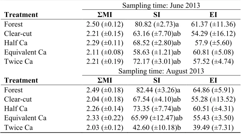
The taxa identified ranged the entire breadth of the p scale (Table 3.1, 3.2); however, c-p 5 taxa were only observed in August samc-ples. Rec-peated measures ANOVA found no
significant differences among the ΣMI or EI indices between treatments (F4, 15 = 1.925, p
= 0.158; F4, 15 = 1.726, p = 0.197, respectively) sampling time (F1, 15 = 0.151, p = 0.703; F1, 15 = 0.223, p = 0.643, respectively) or from time by treatment interactions (F4, 15 = 0.564, p = 0.693; F4, 15 = 0.336, p = 0.844, respectively) (Table 3.4). The SI was the only Maturity Index to show a significant treatment effect: the highest mean SI values
3.2.2 Body Size Spectra
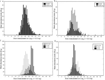
Both the LSDR and ISD models of BSS showed similar patterns for change between the forest and clear-cut treatments at the June sampling. This is seen in the LSDR model via the regression lines, whose slopes were not significantly different from each other (forest slope = -0.579; clear-cut = -0.592) nor were the y-intercepts (forest = 1.934; clear-cut = 1.785); however data did show a slight reduction in the overall mean abundance (Figure 3.2a). In the ISD model, this trend was observed via the slight reduction in both small and large-bodied taxa (Figure 3.3a). Trends in the LSDR model of ash treatments were
unclear. There was an increase of smallbodied taxa in the half Ca treatment (slope = -0.708, intercept = 2.015). However, this did not carry over into the equivalent and twice Ca treatments, which show shallower slopes than all other treatments (slope = -0.305, intercept = 1.512; slope = -0.411, intercept = 1.860, respectively) (Figure 3.2c). Overall, there was a statistically significant difference between treatments in slope (F8, 100 > 100, p
< 0.001) but not intercept (F4, 100 = 0.944, p = 0.441). In the ISD model, an increase in all
body size classes, not just the smaller ones, was observed in the half Ca treatment, whereas a shift towards larger-bodied individual was seen in the other two Ca treatments (Figure 3.3c).
In August samples, the LSDR model produced much different results. The forest community was very low in abundance (intercept = 1.23) and had the regression line with the shallowest slope (slope = -0.093). Abundance in the clear-cut was unexpectedly high as well and the slope was representative of a community with more large-bodied
constituents than the forest community (intercept = 1.66, slope = -0.601) (Figure 3.2b). Results from the ash treatments were also not as expected. The twice Ca community seemed to show an unexpected enrichment effect, with the highest recorded intercept and steepest slope (intercept = 1.673, slope = -0.698). Half and equivalent Ca regressions had shallower slopes indicating the greater presence of larger taxa (intercept = 1.60, slope = -0.428; intercept = 1.387, slope = -0.309, respectively). There was a significant difference between treatment levels in slope (F8, 88 = 2.321, p = 0.026) but not intercept (F4, 88 =
distribution, but similar to the June samples, it shows a reduction in the largest and smallest size classes (Figure 3.3b). However, in the Ca amended soils, the opposite trend was seen in August when compared to June. Smaller body size classes dominated the equivalent and twice Ca treatments, whereas the half Ca treatment was shifted towards larger individuals (Figure 3.3d).
3.3
Wood ash and the nematode community:
molecular assessment using
T
-
RFLP
Table 3.1: Total abundance (per 25 g soil) of each taxon of free-living nematodes collected under forest, clear-cut and the three different wood ash applications from June 2013. Taxa are listed in order of lowest to highest c-p rank.
Taxon (c-p rank) Forest Clear-cut
Half Ca (100g/ha)
Equivalent Ca (200g/ha)
Twice Ca (400g/ha)
Rhabditidae (1) 86 76 62 66 75
Panagrolaimidae (1) 67 34 103 33 42
Acrobeloides (2) 66 130 114 80 92
Cephalobus (2) 0 2 1 1 0
Chiloplacus (2) 0 0 0 1 0
Eucephalobus (2) 2 0 6 0 0
Plectus (2) 54 62 200 86 128
Wilsonema (2) 29 20 101 24 85
Criconema (3) 1 0 0 0 2
Criconemoides (3) 1 0 0 0 0
Hemicycliophora (3) 10 3 16 0 6
Prismatolaimus (3) 1 0 5 2 3
Teratocephalus (3) 57 21 73 5 34
Trichostoma (3) 0 0 1 0 0
Tripyla (3) 5 27 22 10 20
Tylolaimophorus (3) 3 1 1 6 4
Alaimus (4) 72 61 76 22 64
Clarkus (4) 6 4 4 8 11
Epidorylaimus (4) 1 1 2 1 1
Eudorylaimus (4) 38 9 26 14 20
Paramphidelus (4) 27 39 94 9 31
Thonus (4) 4 6 7 2 6
Table 3.2: Total abundance (per 25 g soil) of each taxon of free-living nematodes collected under forest, clear-cut and the three different wood ash applications from August 2013. Taxa are listed in order of lowest to highest c-p rank.
Taxon (c-p rank) Forest Clear-cut
Half Ca (100g/ha)
Equivalent Ca (200g/ha)
Twice Ca (400g/ha)
Rhabditidae (1) 19 53 37 25 56
Panagrolaimidae (1) 18 31 30 20 13
Acrobeloides (2) 7 39 37 43 222
Plectus (2) 35 83 84 59 51
Cephalobus (2) 0 29 17 39 73
Wilsonema (2) 10 15 19 7 14
Eucephalobus (2) 1 2 0 5 24
Fungiotonchium (2) 0 0 3 0 1
Hemicycliophora (3) 10 10 16 7 9
Teratocephalus (3) 4 9 17 3 4
Tylolaimophorus (3) 3 5 1 7 1
Prismatolaimus (3) 0 3 2 9 0
Bastiania (3) 2 5 5 0 1
Tripyla (3) 2 4 2 3 0
Macroposthonia (3) 1 0 0 0 0
Eudorylaimus (4) 13 23 70 23 10
Paramphidelus (4) 16 21 31 9 16
Alaimus (4) 7 26 18 8 5
Thonus (4) 5 9 5 11 2
Clarkus (4) 12 4 7 7 1
Epidorylaimus (4) 1 1 7 2 0
Paravulvus (5) 4 0 0 0 0
Sectonema (5) 1 0 0 0 0
Table 3.3: Mean abundance, richness, diversity and evenness values by treatment from June and August samples. Standard errors are listed in parenthesis.
Sampling time: June 2013
Treatment Abundance (# individuals / 25 g wwt soil)
Richness (# taxa / 25 g wwt soil)
Shannon diversity
(H') Evenness (J')
Forest 160.75 (±61.40) 13.75 (±0.63) 2.18 (±0.04) 0.83 (±0.02)
Clear-cut 142.50 (±66.52) 11.50 (±0.96) 1.94 (±0.11) 0.80 (±0.04)
Half Ca 271 (±187.63) 13.75 (±1.18) 2.16 (±0.07) 0.83 (±0.01)
Equivalent Ca 100 (±24.96) 11.50 (±0.87) 1.98(±0.02) 1.98 (±0.02)
Twice Ca 185 (±145.51) 11 (±1.96) 1.86(±1.13) 1.85 (±0.04)
Sampling time: August 2013
Treatment Abundance (# individuals / 25 g wwt soil) Richness (# taxa / 25 g wwt soil) Shannon diversity (H') Evenness (J')
Forest 42.75 (±19.79) 10.25 (±2.14) 1.93 (±0.17) 0.86 (±0.02)
Clear-cut 94.50 (±34.91) 13.75 (±1.65) 1.99 (±0.10) 0.77 (±0.02)
Half Ca 104.75 (±21.44) 13.50 (±0.87) 2.04 (±0.10) 0.79 (±0.02)
Equivalent Ca 71.50 (±26.88) 12.25 (±1.89) 2.10 (±0.18) 0.85 (±0.04)
Table 3.4: Mean values of the trait-based indices, ΣMI, SI, and EI, as well as abundance by treatment from samples collected in June and August 2013 from the Island Lake Biomass and Harvesting Demonstration area near Chapleau, Ontario. Indices SI and EI are expressed as percentages. Standard errors are listed in parenthesis. Values followed by the same letter in the same column are not significantly different based on Tukey post hoc test among treatments.
Sampling time: June 2013
Treatment ΣMI SI EI
Forest 2.50 (±0.12) 80.82 (±2.73)a 61.37 (±11.36) Clear-cut 2.21 (±0.15) 63.16 (±7.70)ab 54.29 (±16.12) Half Ca 2.29 (±0.11) 68.52 (±2.80)ab 57.9 (±5.60) Equivalent Ca 2.11 (±0.08) 58.63 (±1.21)ab 60.81 (±5.08) Twice Ca 2.21 (±0.19) 72.17 (±3.01)ab 57.52 (±4.74)
Sampling time: August 2013
Treatment ΣMI SI EI
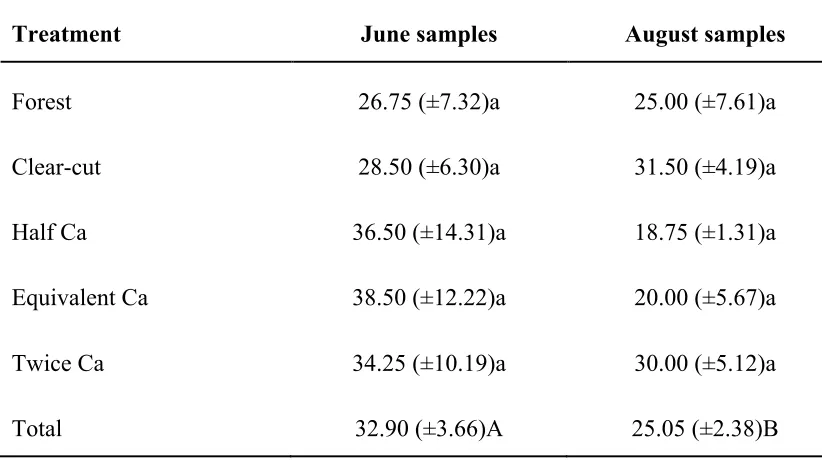
Table 3.5: Mean richness values of OTUs obtained from T-RFLP analyses in June and August sampling. Standard errors are listed in parenthesis. Letters followed by the same letter in the same column are not significantly different based on Tukey post hoc test among treatments (lower case) and time (upper case).
Treatment June samples August samples
Forest 26.75 (±7.32)a 25.00 (±7.61)a
Clear-cut 28.50 (±6.30)a 31.50 (±4.19)a
Half Ca 36.50 (±14.31)a 18.75 (±1.31)a
Equivalent Ca 38.50 (±12.22)a 20.00 (±5.67)a
Twice Ca 34.25 (±10.19)a 30.00 (±5.12)a
Figure 3.1: Weighted c-p triangles (ternary plots) showing the proportional distribution of c-p groups from each replicate of the forest, clear-cut, and ash-amended treatments in relation to the three soil states identified by the MI from June and August samples.
100 90 80 70 60 50 40 30 20 10 0
0 10 20 30 40 50 60 70 80 90
100 0 10 20 30 40 50 60 70 80 90 100 c-p 2 c-p 1 c-p 3-5 Enriched Structured Basal 100 90 80 70 60 50 40 30 20 10 0
0 10 20 30 40 50 60 70 80 90
Figure 3.2: The nematode community as seen through the LSDR model of BSS using dry weight (ng) and abundance on a log10 scale of forest and clear-cut treatments in A) June and B) August, and one-half, equivalent, and twice Ca amendment in C) June and D) August. Regression lines were fit using the 75th quartile.
−0.5 0.0 0.5 1.0 1.5 2.0 2.5 Log (mass) Log (ab undance) 0.0 0.5 1.0 1.5 2.0 2.5 Forest
Clear−cut
A
−0.5 0.0 0.5 1.0 1.5 2.0 2.5 0.0 0.5 1.0 1.5 2.0 2.5 Log (mass) Log (ab undance)
2.0 x Calcium 0.5 x Calcium 1.0 x Calcium
C
−0.5 0.0 0.5 1.0 1.5 2.0 2.5 Log (mass) Log (ab undance) 0.0 0.5 1.0 1.5 2.0 2.5 Forest
Clear−cut
B
−0.5 0.0 0.5 1.0 1.5 2.0 2.5 0.0 0.5 1.0 1.5 2.0 2.5 Log (ab undance)
2.0 x Calcium 0.5 x Calcium 1.0 x Calcium
D
Figure 3.3: The nematode community as seen through the ISD model of BSS with mean body size classes based on Log2 plus 0.5 ng
and abundance of forest and clear-cut treatments in A) June and B) August, and one-half, equivalent, and twice Ca amendment in C) June and D) August.
1 5 9 13 17 21 25 29 33 37 41 45 49 53 Size class (based on Log2 x + 0.5 ng)
0 10 20 30 40 50 60 70 80 90
Mean abundance (indiv./25 g)
Forest Clear-cut
1 5 9 13 17 21 25 29 33 37 41 45 49 53 Size Class (based on Log2 x + 0.5 ng)
0 20 40 60 80 100 120 140 160 180 200
Mean abundance (indiv./25 g)
0.5 x Ca 1 x Ca 2 x Ca
1 5 9 13 17 21 25 29 33 37 41 45 49 53 Size class (based on Log2 x + 0.5 ng)
0 10 20 30 40 50 60
Mean abundance (indiv./25 g)
Forest Clear-cut
1 5 9 13 17 21 25 29 33 37 41 45 49 53 0 20 40 60 80 100 120
0.5 x Ca 1 x Ca 2 x Ca
Mean abundance (indiv./25 g)
Size class (based on Log2 x + 0.5 ng)
A B
4
Discussion
4.1
Response of the nematode community to
clear-cutting
4.1.1 Morphological measures of nematode communities
The nematode community appeared to be resistant to clear-cutting disturbance in this study. Although nematodes have been frequently observed to negatively respond to clear-cutting, these responses are hardly uniform. Changes in the nematode community after clear-cutting, if they are present, likely stem from alterations in the physical
characteristics of the soil, including moisture and temperature regimes, as well as alterations in physical structure (Marshall, 2000; Sohlenius, 2002). Gross abundances of nematodes often decrease following clear-cutting (Huhta et al.,1967; Panesar et al., 2000) yet species richness (Hánĕl, 2004) and diversity indices are often unaffected, especially in the time shortly following harvesting (Panesar et al., 2000; Forge & Simard, 2001). Such a situation often arises following significant reductions in relative
abundances of the most abundant taxa, thereby increasing diversity and evenness values (Forge & Simard, 2001), yet richness stays roughly the same. This was not apparent in the present study with the same three groups (Plectus sp., Acrobeloides sp., Rhabditidae sp.) remaining the most abundant at both sample times, and diversity indices not
changing significantly. Rather I found that lower relative abundances of some groups (e.g. Alaimus sp.) were countered with greater abundances in other groups (e.g.
Though not expected, a lack of major change in richness and abundance of nematodes following forest harvesting is not altogether unusual; it has been observed with some frequency in the literature (Marshall, 2000; Hánĕl, 2004), and there are several factors that may contribute to this lack of change. For instance, Huhta et al. (1967), who are often cited as evidence for the negative effects of clear-cutting on nematodes, suggest that non-significant changes can arise due to greater pressure from the so-called
“prevailing situation” of the system than disturbance itself. Though vague, this phrase can be understood to mean the host of abiotic factors present in a system that leads to high variability and obscures treatment effects. Indeed, Huhta et al. (1967) later note that the nematode communities they studied displayed a greater response to seasonality than to clear-cutting itself. Although the present study did not show a significant seasonality of the nematode communities, this could be due to sampling occurring at the beginning and middle of the growing season, which generally are not much different from one another (Panesar et al., 2000).
Though microclimate variation following clear-cutting has been extensively considered in the succession of soil fauna (Siira-Pietikäinen & Haimi, 2009) there were no apparent differences in the physical properties of the soil at the time of June sampling. However, this was early in the season. Removal of the canopy within the clear-cut would increase solar radiation and precipitation, and thereby increase soil temperature and temperature fluctuations (Keenan & Kimmins, 1993), as well as soil moisture