Adaptive Security of Constrained PRFs
Georg Fuchsbauer1, Momchil Konstantinov2, Krzysztof Pietrzak1?, and Vanishree Rao3
1
IST Austria,{gfuchsbauer,pietrzak}ist.ac.at
2
London School of Geometry and Number Theory, UK 3 UCLA, USA
Abstract. Constrained pseudorandom functions have recently been introduced independently by Boneh and Waters (Asiacrypt’13), Kiayias et al. (CCS’13), and Boyle et al. (PKC’14). In a standard pseudorandom function (PRF) a keyKis used to evaluate the PRF on all inputs in the domain. Constrained PRFs additionally offer the functionality to delegate “constrained” keysKS which allow to evaluate the PRF only on a subsetS of the domain.
The three above-mentioned papers all show that the classical GGM construction (J.ACM’86) of a PRF from a pseudorandom generator (PRG) directly yields a constrained PRF where one can compute constrained keys to evaluate the PRF on all inputs with a given prefix. This constrained PRF has already found many interesting applications. Unfortunately, the existing security proofs only show selective security (by a reduction to the security of the underlying PRG). To achieve full security, one has to use complexity leveraging, which loses an exponential factor 2N in security, whereN is the input length.
The first contribution of this paper is a new reduction that only loses a quasipolynomial factorqlogN, whereqis the number of adversarial queries. For this we develop a new proof technique which constructs a distinguisher by interleaving simple guessing steps and hybrid arguments a small number of times. This approach might be of interest also in other contexts where currently the only technique to achieve full security is complexity leveraging.
Our second contribution is concerned with another constrained PRF, due to Boneh and Waters, which allows for constrained keys for the more general class of bit-fixing functions. Their security proof also suffers from a 2N loss, which we show is inherent. We construct a meta-reduction which shows that any “simple” reduction of full security from a non-interactive hardness assumption must incur an exponential security loss.
Keywords: Constrained PRF, complexity leveraging, full security, meta-reduction.
1 Introduction
PRFs. Pseudorandom functions (PRFs) were introduced by Goldreich, Goldwasser and Micali [GGM86]. A PRF is an efficiently computable keyed function F: K × X → Y, where F(K,·), instantiated with a random keyK ← K∗ , cannot be distinguished from a function randomly chosen from the set of all functions
X → Y with non-negligible probability.
Constrained PRFs. Recently, the notion of constrained PRFs (CPRFs) was introduced independently by Boneh and Waters [BW13], Boyle, Goldwasser and Ivan [BGI14] and Kiayias, Papadopoulos, Trian-dopoulos and Zacharias [KPTZ13].4
A constrained PRF is defined with respect to a set system S ⊆ 2X and supports the functionality to “delegate” (short) keys that can only be used to evaluate the function F: K × X → Y on inputs specified by a subset S ∈ S. Concretely, there is a “constrained” keyspace Kc and additional algorithms
F.constrain:K × S → Kc and F.eval:Kc× X → Y, which for all K ∈ K, S ∈ S, x ∈ S and KS ←
F.constrain(K, S), satisfyF.eval(KS, x) =F(K, x) if x∈S and F.eval(KS, x) =⊥otherwise. ?Research supported by ERC starting grant (259668-PSPC)
4
The GGM and the Boneh-Waters construction. All three papers [BW13,BGI14,KPTZ13] show that the classical GGM construction [GGM86] of the PRF GGM:{0,1}λ × {0,1}N → {0,1}λ from a
length-doubling pseudorandom generator (PRG)G:{0,1}λ → {0,1}2λ directly yields a constrained PRF,
where for any key K and input prefix z ∈ {0,1}≤N, one can generate a constrained key K
z that allows
to evaluate GGM(K, x) for any x with prefix z. This simple constrained PRF has found many appli-cations; apart from those discussed in [BW13,BGI14,KPTZ13], it can be used to construct so-called “punctured” PRFs, which are a key ingredient in almost all the recent proofs of indistinguishability obfuscation [SW14,BCPR13,HSW14].
Boneh and Waters [BW13] construct a constrained PRF for a much more general set of constraints, where one can delegate keys that fix any subset of bits of the input (not just the prefix, as in GGM). The construction is based on leveled multilinear maps [GGH13] and its security is proven under a generalization of the decisional Diffie-Hellman assumption.
Security of constrained PRFs. The security definition for standard PRFs is quite intuitive. One considers two experiments: the “real” experiment and the “random” experiment, in both of which an adversaryAgets access to an oracleO(·) and then outputs a bit. In the real experiment O(·) implements the PRFF(K,·) using a random key; in the random experimentO(·) implements a random function. The PRF is secure if every efficient Aoutputs 1 in both experiments with (almost) the same probability.
Defining the security of constrained PRFs requires a bit more thought. We want to give an adversary access not only toF(K,·), but also to the constraining functionF.constrain(K,·). But now we cannot expect the values F(K,·) to look random, as an adversary can always ask for a keyKS←F.constrain(K, S) and
then for anyx∈S check whether F(K, x) =F.eval(KS, x).
Instead, security is formalized by defining the experiments in two phases. In the first phase of both experiments the adversary gets access to the same oracles F(K,·) and F.constrain(K,·). The experiments differ in a second phase, where the adversary chooses some challenge queryx∗. In the real experiment the adversary then obtainsF(K, x∗), whereas in the random experiment she gets a random value. Intuitively, when no efficient adversary can distinguish these two games, this means that the outputs ofF(K,·) look random on all points that the adversary cannot compute by herself using the constrained keys she has received so far.
Selective vs. full security. In the above definition we let the adversary choose the challenge input x∗ after she gets access to the oracles. This is the notion typically considered, and it is called “full security” or “adaptive security”. One can also consider a weaker “selective security” notion, where the adversary must choosex∗ before getting access to the oracles.
The reason to consider selective security notions, also for other objects like identity-based encryp-tion [BF01,BB04,AFL12], is that it is often much easier to achieve. Although there exists a simple generic technique called “complexity leveraging”, which translates any selective security guarantee into a security bound for full security, this technique (which really just consists of guessing the challenge) typically loses an exponential factor (in the length of the challenge) in the quality of the reduction, often making the resulting security guarantee meaningless for practical parameters.
1.1 Our Contributions
negative result, showing that for a large class of reductions, an exponential loss is necessary. We now elaborate on these results.
A quasipolynomial reduction for GGM. To prove full security ofGGM:{0,1}λ× {0,1}N → {0,1}λ,
the “standard” proof proceeds in two steps (we give a precise statement in Proposition 3).
1. A guessing step (a.k.a. complexity leveraging), which reduces full to selective security. This step loses an exponential factor 2N in the input lengthN.
2. Now one applies a hybrid argument which loses a factor 2N.
Readers not familiar with hybrid arguments can find a simple application of this technique in Appendix A. The above two steps transform an adversary Af that breaks the full security ofGGM with advantage into a new adversary that breaks the security of the underlying pseudorandom generator G (used to construct the GGMfunction) with advantage /(2N·2N). As a consequence, even if one makes a strong exponential hardness assumption on the PRGG, one must use a PRG whose domain isΘ(N) bits in order to get any meaningful security guarantee.
The reason for the huge security loss is the first step, in which one guesses the challengex∗∈ {0,1}N
the adversary will choose, which is correct with probability 2−N. To avoid this exponential loss, one must thus avoid guessing the entire x∗. Our new proof also consists of a guessing step followed by a hybrid argument.
1. A guessing step, where (for some `) we guess which of the adversary’s queries will be the first one that agrees with x∗ in the first `positions.5 This step loses a factor q, which denotes the number of queries made by the adversary.
2. A hybrid argument which loses a constant factor 3.
The above two steps only lose a factor 3q. Unfortunately, after one iteration of this approach we do not get a distinguisher forGright away. At a high level, these two steps achieve the following: We start with two games which in some sense are at distanceN from each other, and we end up with two games which are at distanceN/2. We can iterate the above processn:= logN times to end up with games at distance N/2n = 1. Finally, from any distinguisher for games at distance 1 we can get a distinguisher for the
PRGGwith the same advantage. Thus, starting from an adversary against the full security ofGGMwith advantage, we get a distinguisher for the PRG with advantage/(3q)logN.
We can optimize this by combining this approach with the original proof, and therby obtain a quasipolynomial loss of 2qlogq·(3q)logN−log logq. To give some numerical example, let the input length be N = 210 = 1024 and the number of queries be q= 232. Then we get a loss of 2qlogq·(3q)logN−log logq= 2·232·32·(3·232)10−5= 2198·35≤2206, whereas complexity leveraging loses 2N2N = 21035.
Although our proof is somewhat tailored to theGGMconstruction, the general “fine-grained” guessing approach outlined above might be useful to improve the bounds for other constructions (like CPRFs, and even IBE schemes) where currently the only proof technique that can be applied is complexity leveraging.
A lower bound for the Boneh-Waters CPRF and Hofheinz’s construction. We then turn our attention to the bit-fixing constrained PRF by Boneh and Waters [BW13]. For this construction too, complexity leveraging—losing an exponential factor—is the only known technique to prove full security. We give strong evidence that this is inherent (even when the construction is only used as a prefix-fixing CPRF).
Concretely, we prove that every “simple” reduction (which runs the adversary once without rewinding; see Section 5.2) of the full security of this scheme from any decisional (and thus also search) assumption
must lose an exponential factor. Our proof is a so-called meta-reduction [BV98,Cor02,FS10], showing that any reduction that breaks the underlying assumption when given access to any adversary that breaks the CPRF, could be used to break the underlying assumption without the help of an adversary.
This impossibility result is similar to existing results, the closest one being a result of Lewko and Wa-ters [LW14] ruling out security proofs without exponential loss for so-called “prefix-encryption” schemes (which satisfy some special properties). Other related results are those of Coron [Cor02] and Hofheinz et al. [HJK12], which show that security reductions for certain signature schemes must lose a factor polynomial in the number of signing queries.
The above impossibility proofs are for public-key objects, where a public key uniquely determines the input/output distribution of the object. This property is crucially used in the proof, wherein one first gets the public key and then runs the reduction, rewinding the reduction multiple times to the point right after the public key has been received.
As we consider a secret-key primitive, the above approach seems inapplicable. We overcome this by observing that for the Boneh-Waters CPRF we can initially make some fixed “fingerprint” queries, which then uniquely determine the remaining outputs. We then use the responses to these fingerprint queries instead of a public key as in [LW14].
Hofheinz [Hof14] has (independently and concurrently with us) investigated the adaptive security of bit-fixing constrained PRFs. He gives a new construction of such PRFs which is more sophisticated than the Boneh-Waters construction, and for which he can give a security reduction that only loses a polynomial factor. The main tool that allows Hofheinz to overcome our impossibility result is the use of a random oracle H(·). Very informally, instead of evaluating the PRF on an inputX, it is evaluated on H(X) which forces an attacker to make every query X explicit. Unfortunately, this idea does not work directly as it destroys the structure of the preimages, and thus makes the construction of short delegatable keys impossible. Hofheinz deals with this problem using several other ideas.
2 Preliminaries
For a ∈N, we let [a] :={1,2, . . . , a} and [a]0 := {0,1, . . . , a}. By {0,1}≤a =Si≤a{0,1}i we denote the
set of bitstrings of length at mosta, including the empty string∅. ByUa we denote the random variable
with uniform distribution over {0,1}a. We denote sampling s uniformly from a set S by s ∗
← S. We let xky denote the concatenation of the bitstrings x and y. For sets X,Y, we denote by F[X,Y] the set of all functionsX → Y; moreover,F[a, b] is short forF[{0,1}a,{0,1}b]. Forx∈ {0,1}∗, we denote by x
i the
i-th bit ofx, and by x[i . . . j] the substringxikxi+1k. . .kxj.
Definition 1 (Indistinguishability). Two distributions X and Y are (, s)-indistinguishable, de-noted X ∼(,s) Y, if no circuit D of size at most s can distinguish them with advantage greater than , i.e.,
X ∼(,s)Y ⇐⇒ ∀D,|D| ≤s: Pr[D(X) = 1]−Pr[D(Y) = 1] ≤ .
X∼δ Y denotes that the statistical distance of X and Y is δ (i.e., X∼(δ,∞) Y), andX ∼Y denotes that
they have the same distribution.
Definition 2 (PRG). An efficient function G: {0,1}λ → {0,1}2λ is an (, s)-secure (length-doubling) pseudorandom generator (PRG) if
Definition 3 (PRF). A keyed functionF:K × X → Y is an (, s, q)-secure pseudorandom function
if for all adversaries A of size at mosts making at most q oracle queries
Pr
K←K∗ [AF(K,
·) →1]−Pr
f←F∗ [X,Y][A
f(·)→1] ≤ .
Constrained pseudorandom functions. Following [BW13], we say that a function F:K × X → Y is a constrained PRF for a set systemS ⊆2X, if there is a constrained-key space Kc and algorithms
F.constrain:K × S → Kc and F.eval:Kc× X → Y ,
which for all K∈ K,S ∈ S,x∈S and KS ←F.constrain(K, S) satisfy
F.eval(KS, x) =
F(K, x) ifx∈S
⊥ otherwise .
That is, F.constrain(K, S) outputs a key KS that allows evaluation of F(K,·) on allx∈S.
Informally, a constrained PRF F is secure, if no efficient adversary can distinguish F(K, x∗) from random, even given access to F(K,·) andF.constrain(K,·) which he can query on all x 6=x∗ and S ∈ S
wherex∗ 6∈S, respectively. We will always assume thatS contains all singletons, i.e.,∀x∈ X : {x} ∈ S; this way we do not have to explicitly give the adversary access to F(K,·), as F(K, x) can be learned by querying forKx ←F.constrain(K,{x}) and computingF.eval(Kx, x).
We distinguish between selective and full security. In the selective security game the adversary must choose the challenge x∗ before querying the oracles. Both games are parametrized by the maximum number q of queries the adversary makes, of which the last query is the challenge query.
ExpselCPRF(A,F, b, q)
K ∗
← K, Sˆ:=∅, c:= 0
x∗←A AO(·)
C0← Y∗ , C1:=F(K, x∗)
AgetsCb ˜
b←A
ifx∗∈Sˆ, return 0 return ˜b
ExpfullCPRF(A,F, b, q)
K ∗
← K, Sˆ:=∅, c:= 0
AO(·) x∗←A
C0← Y∗ , C1:=F(K, x∗)
AgetsCb ˜b←A
ifx∗∈Sˆ, return 0 return ˜b
OracleO(S)
ifc=q−1, return⊥
c:=c+ 1 ˆ
S:= ˆS ∪S
KS←F.constrain(K, S) returnKS
Foratk∈ {sel,full} we defineA’s advantage as
AdvatkF (A, q) = 2Prb←{∗
0,1}[ExpatkCPRF(A,F, b, q) =b]−12
(1)
and denote with
AdvatkF (s, q) = maxA,|A|≤sAdvatkF (A, q) the advantage of the bestq-query adversary of size at mosts.
Definition 4 (Selective and full security of CPRFs). A constrained PRF F is
– selectively (, s, q)-secure ifAdvselF (s, q)≤ and
K∅
K0
K00
K000 K001
K01
K010 K011
K1
K10
K100 K101
K11
K110 K111
Fig. 1.Illustration of the GGM PRF. Every left childKzk0of a nodeKz is defined as the first half ofG(Kz), the right child
Kzk1 as the second half. The circled node corresponds toGGM(K∅,010).
Remark 1 (CCA1 vs. CCA2 security). In the selective and full security notion, we assume that the chal-lenge queryx∗ is only made at the very end, whenAhas no longer access to the oracle (this is reminiscent of CCA1 security). All our positive results hold for stronger notions (reminiscent to CCA2 security) where
Astill has access to O(·) after making the challenge query, but may not query it on any S wherex∗ ∈S.
Remark 2 (Multiple challenge queries). We only allow the adversary one challenge query. As observed in [BW13], this implies security against anyt >1 challenge queries, losing a factor oftin the distinguishing advantage, by a standard hybrid argument.
Using what is sometimes called “complexity leveraging”, one can show that selective security implies full security: given an adversary A against full security, we construct a selective adversary B, which at the beginningguesses a challengex∗ and outputs it, then runsAand aborts if the challenge thatAeventually outputs is different fromx∗. The distinguishing advantage drops thus by a factor of the domain size|X |. The following is proved in Appendix B.1.
Lemma 1 (Complexity leveraging). If a constrained PRF F: K × X → Y is (, s, q)-selectively
secure then it is(|X |, s0, q)-fully secure (where s0 =s−O(log|X |)), i.e.,
AdvfullF (s0, q)≤ |X | ·AdvselF (s, q) .
3 The GGM Construction
The GGM construction, named after its inventors Goldreich, Goldwasser and Micali [GGM86], is a keyed function GGMG:{0,1}λ × {0,1}∗ → {0,1}λ defined by any length-doubling pseudorandom generator
G:{0,1}λ→ {0,1}2λ recursively as
GGM(K∅, X) =KX , where ∀Z ∈ {0,1}≤N−1: KZk0kKZk1=G(KZ) (2)
(cf. Figure 1). In [GGM86] it is shown that when the inputs are restricted to{0,1}N thenGGMGis a secure PRF if Gis a secure PRG. Their proof is one of the first applications of the so-called hybrid argument.6 The proof loses a factor of q·N in distinguishing advantage (where q is the number of queries).
Proposition 1 (GGM is a PRF [GGM86]). If G:{0,1}λ → {0,1}2λ is an (
G, sG)-secure PRG then
(for any N, q) GGMG:{0,1}λ× {0,1}N → {0,1}λ is an (, s, q)-secure PRF with
=G·q·N and s=sG−O(q·N· |G|) .
We will not give a proof of this proposition here; however it follows from Proposition 2 below, for which we give a proof sketch. In his book [Gol01] Goldreich presents several generalizations of GGM, including a variant which is secure even if we allow the entire domain{0,1}∗as inputs. Here, we’d like to mention that
the original GGM construction is a secure “prefix-free” PRF as defined below. The reason for presenting this variant of GGM here is so we can later, in Remark 3, discuss why this variant of GGM does not
already imply security of GGM as a constrained PRF. Instead of the number q of points queried by the adversary, the security of a prefix-free PRF with domain {0,1}∗ is parametrized by the sum m of the bitlengths of all queries.
Definition 5 (PF-PRF). A keyed functionF:K × {0,1}∗ → Y is an (, s, m)-secureprefix-free
pseu-dorandom function(PF-PRF) if for all adversariesAof size at mostsmaking queries of total bitlength at mostm, but where no query can be a prefix of another query,
PrK∗
←K[AF(K,
·)→1]−Pr
f←F∗ [{0,1}∗,Y][Af(·)→1]
≤ .
Proposition 2 (GGM is a PF-PRF). If G:{0,1}λ → {0,1}2λ is an (
G, sG)-secure PRG then (for
anym)GGMG:{0,1}λ× {0,1}∗→ {0,1}λ is an (, s, m)-secure PF-PRF with
=G·m and s=sG−O(m· |G|) .
We prove this proposition in Appendix B.2. Note that if we drop the restriction that queries must be prefix-free, the construction is trivially insecure, as fromy=GGMG(K, x) one can computey0=GGMG(K, xkz) for anyz, thusy0 is not pseudorandom given y. Also note that restricting the domain to{0,1}N, we get
m=q·N, as stated in Proposition 1.
3.1 GGM is a Constrained PRF
As observed recently by three different works independently [BW13,BGI14,KPTZ13], the GGM construc-tion can be used as a constrained PRF for the set system Spre of sets of inputs with common prefixes, defined as
Spre={Sp : p∈ {0,1}≤N} , where Sp ={pkz : z∈ {0,1}N−|p|} .
Thus, given a key Kp for the set Sp, one can evaluateGGMG(K,·) on all inputs with prefix p. Formally,
the constrained PRF with key K=K∅ is defined using (2) as follows:
GGMG.constrain(K∅, p) =GGMG(K∅, p) =Kp and GGMG.eval(Kp, x=pkz) =GGMG(Kp, z) =Kx .
An interior nodeKp in Figure 1 is thus the constrained key for the setSp.
Remark 3. One might be tempted to think that the fact that GGM is a PF-PRF (Proposition 2), together with the fact that constrained-key derivation is simply the GGM function itself, already implies that it is a secure constrained PRF. Unfortunately, this is not sufficient, as the (selective and full) security notions for constrained PRFs do allow queries that are prefixes of previous queries.
Remark 4. In the proof of Proposition 3 and Theorem 1 we will slightly cheat, as in the security game whenb= 0 (i.e., when the challenge output is random) we not only replace the challenge outputKx∗, but
also its siblingKx∗[1...N−1]x∗
N, with a random value. Thus, technically this only proves security for inputs
of lengthN−1 (as we can e.g. simply forbid queriesxk0, x∈ {0,1}N−1, in which case it is irrelevant what the sibling is, as it will never be revealed). The proofs without this cheat require one extra hybrid, which requires a somewhat different treatment than all others hybrids and thus would complicate certain proofs and definitions. Hence, we chose to not include it. The bounds stated in Proposition 3 and Theorem 1 are the bounds we getwithout this cheat.
Proposition 3. IfG:{0,1}λ → {0,1}2λ is an(
G, sG)-secure PRG then (for anyN, q)GGMG:{0,1}N →
{0,1}λ is a constrained PRF forS
pre which is
1. selectively (, s, q)-secure, with
=G·2N and s=sG−O(q·N· |G|) ;
2. fully (, s, q)-secure, with
=G·2N2N and s=sG−O(q·N· |G|) .
Full security as stated in Item2. of the proposition follows from selective security (Item1.) by complexity leveraging as explained in Lemma 1. To prove selective security, we let H0 be the real game for selective security and letH2N−1 be the random game, that is, whereKx∗ is random. We then define intermediate
hybrid games H1, . . . , H2N−2 by embedding random values along the path to Kx∗. (See Figure 5 in
Appendix A for an illustration.) In particular, in hybridHi, for 1≤i≤N, the nodesK∅, Kx∗
1, . . . , Kx∗[1...i]
are random and forN+ 1≤i≤2N−1 the nodesK∅, Kx∗1, . . . , Kx∗[1...2N−1−i]andKx∗ are random. Thus
two consecutive games Hi, Hi+1 differ in one node that is real in one game and random in the other, and the parent of that node is random, meaning we can embed a PRG challenge. From any distinguisher for two consecutive games we thus get a distinguisher for the PRG G with the same advantage. (See Appendix B.3 for a formal proof.)
This hybrid argument only loses a factor 2N in distinguishing advantage, but complexity leverag-ing loses a huge factor 2N. In the next section we show how to prove full security avoiding such an exponential loss.
4 Full Security with Quasipolynomial Loss
Theorem 1. If G:{0,1}λ → {0,1}2λ is an (
G, sG)-secure PRG then (for any N, q) GGMG:{0,1}N →
{0,1}λ is a fully(, s, q)-secure constrained PRF forS
pre, where
=G·(3q)logN and s=sG−O(q·N · |G|) .
At the end of this section we will sketch how to combine the proof of this theorem with the standard complexity leveraging proof from Proposition 3 to get a smaller loss of =G·2qlogq·(3q)logN−log logq.
Proof idea. We can view the real and the random game for CPRF security as having distanceN, in the sense that from the only node in which they differ (which is the challenge nodeKx∗) we have to walk up
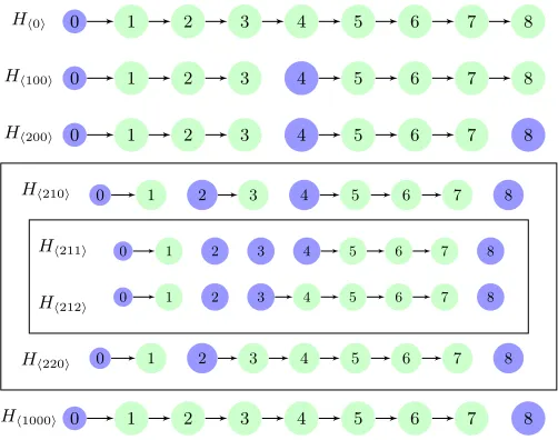
As outlined in Section 1.1, our goal is to halve that distance. For this, we could define two intermediate hybrids which are defined as the real and the random games, except that the node half way down the path tox∗, i.e.,Kx∗[1...N/2], is a random node. This is illustrated in Figure 2, where a row depicts the path from
the root (labeled ‘0’) to x∗ (labeled ‘8’) and where blue nodes correspond to random values. The path at the top of the figure is the real game and the one at the bottom is the random game (ignore anything in the boxes for now), and the intermediate hybrids are the 2nd and the 3rd path. Of these 4 hybrids, each pair of consecutive hybrids has the following property: they differ in one node and its distance to the closest random node above is N/2.
There is a problem with this approach because the intermediate hybrid games we have just constructed are not even well-defined, as the valuex∗[1. . . N/2] is only known when the adversary makes his challenge query. This is also the case forx∗itself, butKx∗only needs to be computed oncex∗ is queried; in contrast,
Kx∗[1...N/2] could have been computed earlier in the game, if the value of some constrained-key query is
a descendant of it. In order to avoid possible inconsistencies, we do the following: we guess which of the adversary’s queries will be the first one with a prefix x∗[1. . . N/2]. As there are at most q queries and there always exists a query with this property (at latest the challenge query itself), the probability of guessing correctly is 1/q. If we guess correctly then the node x∗[1. . . N/2] is known precisely when the valueKx∗[1...N/2] is computed for the first time and we can correctly simulate the game. If our guess was
wrong, we abort.
Assuming an attacker can distinguish between the real and the random game, there must be two consecutive hybrids of the 4 hybrids that it can distinguish with at least one third of his original advantage. Between these two hybrids, which differ in one noded, we can then embed two new intermediate hybrids, which have a random value half way betweendand the closest random node above (cf. the outer box in Figure 2). We continue to do so until we reach two hybrids where there is a random node immediately above the differing node. A distinguisher between two such games can then be used to break the PRG.
Neighboring sets with low weight. Before starting with the proof, we introduce some notation. It will be convenient to work with ternary numbers, which we represent as strings of digits from {0,1,2}
within angular brackets h. . .i. We denote repetition of digits as 0n= 0. . .0 (n times). Addition will also
be in ternary, e.g., h202i+h1i=h210i.
Let N = 2n be a power of 2. In the proof of Theorem 1 we will construct 3n+ 1 subsets Sh0i, . . . ,
Sh10ni ⊂ {0, . . . , N}. These sets will define the positions in the path to the challenge where we make random guesses in a particular hybrid. The following definition measures how “close” sets (that differ in one element) are and will be useful in defining neighboring hybrids.
Definition 6 (Neighboring sets). Fork∈N+, two setsS,S0 ⊂
N0 are k-neighboring if
1. S∆S0 := (S ∪ S0)\(S ∩ S0) ={d} for some d∈N0, i.e., they differ in exactly one element d.
2. d−k∈ S.
3. ∀i∈[k−1] : d−i6∈ S.
We define the first set (with index 0 =h0i) and the and last set (with index 3n=h10ni) as
Sh0i:={0} and Sh10ni:={0, N} . (3)
(They will correspond to the real game, where only the root at depth ‘0’ is random, and the random game, where the value for x∗ at depth N is random too.) The remaining intermediate sets are defined recursively as follows. For`= 0, . . . , n, we define the`-th level of sets to be all the sets of the formSh?0n−`i
Hh0i
Hh100i
Hh200i
Hh1000i
Hh210i
Hh220i
Hh211i
Hh212i
0 1 2 3 4 5 6 7 8
0 1 2 3 4 5 6 7 8
0 1 2 3 4 5 6 7 8
0 1 2 3 4 5 6 7 8
0 1 2 3 4 5 6 7 8
0 1 2 3 4 5 6 7 8
0 1 2 3 4 5 6 7 8
0 1 2 3 4 5 6 7 8
Fig. 2.Concrete example (n= 3) illustrating the iterative construction of hybrids in Theorem 1.
Let SI,SI0 be two consecutive level-`sets, by which we mean thatI0 =I +h10n−`i. By construction,
these sets will differ in exactly one element {d} (i.e., SI 6= SI0; and SI∪ {d} = SI0 or SI0 ∪ {d} = SI).
Then the two level-(`+ 1) sets between the level-`setsSI,SI0 are defined as SI+h10
n−(`+1)i:=SI∪ {d− N
2`+1} and SI0−h10
n−(`+1)i:=SI0 ∪ {d− N
2`+1} . (4)
A concrete example forN = 2n= 23 = 8 is illustrated in Figure 2 (where the blue nodes ofHI correspond
toSI).
An important fact we will use is that consecutive level-`sets are (N/2`)-neighboring (see Definition 6);
in particular, consecutive level-nsets (the 4 lines in the box in Figure 2 illustrate 4 consecutive sets) are thus 1-neighboring, i.e.,
∀I ∈ {h0i, . . . ,h2ni}: SI∆SI+h1i ={d} and d−1∈ SI . (5)
Proof of Theorem 1. Below we prove two lemmata (2 and 3) concerning the games defined in Figure 3, from which the theorem follows quite immediately. As the games and the lemmata are rather technical, we first intuitively explain what is going on, going through a concrete example as illustrated in Figure 2. To prove the theorem, we assume that there exists an adversary Af that breaks the full security of
GGMG with some advantage , and from this, we want to construct a distinguisher forG with advantage at least/(3q)n, wheren= logN. Like in the proof of Proposition 3, we can think of the two games that
Af distinguishes as the games where we let Af query GGMG, but along the path from the root K∅ down
to the challengeKx∗ the nodes are either computed by Gor they are random values. The position of the
random values are defined by the setSh0i={0}for the real game and bySh10ni ={0, N} for the random game: in both cases the root K∅ is random, and in the latter game the final output Kx∗ is also random.
We call these two games Hh∅0i and Hh∅10
ni, and they correspond to the games defined in Figure 3 with
P =∅, and I =h0i and h10ni, respectively). As just explained, they satisfy
Hh∅0i∼ExpfullCPRF(Af,GGMG,0, q) and Hh∅10ni∼Exp
full
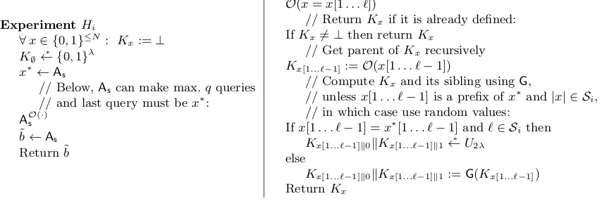
ExperimentHIP
//I∈ {h0i, . . . ,h10ni}
//P={p1, . . . , pt} ⊆ {1, . . . , N−1} //SI ⊆ P ∪ {0, N},SI as in eq. (3) and (4). ∀x∈ {0,1}≤N: K
x:=⊥
K∅
∗ ← {0,1}λ
// Initialize counters: ∀j= 1. . . N−1 : cj= 0
// Make a random guess for each // element inP={p1, . . . , pt}: ∀j∈[t] : qpj
∗ ←[q]
// BelowAf can make exactlyqdistinct
// oracle queriesx1, . . . , xq. The last (chal-// lenge) queryxq=x∗ must be in{0,1}N.
AOf (·)
˜b←A
f
// Only if guessesqp1, . . . , qpt were
// correct, return ˜b, otherwise return 0: If∀p∈ P: x∗[1. . . p−1] =zp−1 then
return ˜b
Else return 0
O(x=x[1. . . `])
// ReturnKxif it is already defined: ifKx6=⊥then returnKx
// Get parent ofKxrecursively:
Kx[1...`−1]:=O(x[1. . . `−1])
// Increase counter for level`−1:
c`−1=c`−1+ 1
// ComputeKxand its sibling usingG, unless its parent //Kx[1...`−1]is a node which we guessed will be on the // path fromK∅andKx∗ and as`∈ P we must use a // random value at this level; OR this is the challenge // queryxq=x∗andN∈ SI, which means the answer // to the challenge is random:
If (`∈ P andc`−1=q`−1) OR (x=xq andN∈ SI)
Kx[1...`−1]k0kKx[1...`−1]k1 ∗ ←U2λ
// Store this node to check if guess was correct later:
z`−1=x[1. . . `−1] else
Kx[1...`−1]k0kKx[1...`−1]k1:=G(Kx[1...`−1])
ReturnKx
Fig. 3.Definition of the hybrid games from the proof of Theorem 1. The setsSI are as in Equations (3) and (4). The hybrid
HIPis defined like the full security game of aq-query adversaryAfagainst the constrained PRFGGMG, but where we “guess”,
for any value inp∈ P, at which point in the experiment the node at depthpon the path from the rootK∅to the challenge
Kx∗is computed (concretely, the guess is that it’s thecp−1th time we compute the children of anp−1 level node, we define theplevel nodeKx∗[1...`] on the path). At a subset of these points, namelySI, we embed random values. The final output is 0 unless all guesses were correct, in which case we forwardAf’s output.
Thus, ifAf breaks the full security ofGGMG with advantagethen
Pr[Hh∅0i= 1]−Pr[Hh∅10
ni= 1]
≥ . (6)
In the proof of Proposition 3 we were able to “connect” the real and random experimentsH0 and H2N−1 via intermediate hybrids H1, . . . , H2N−2, such that from a distinguisher for any two consecutive hybrids we can build a distinguisher forG with the same advantage.
We did this by using random values (instead of applying G) in some steps along the path from the rootK∅ to the challengeKx∗. Here we cannot use the same approach to connectH∅
h0iandH ∅
h10ni, as these
games consider full (and not selective) security, where we learn x∗ only at the very end, and thus “the path tox∗” is not even defined until the adversary makes the challenge query.
We could reduce the problem from the full to the selective setting by guessingx∗ at the beginning like in the proof of Lemma 1, but this would lose a factor 2N, which is what we want to avoid.
Instead of guessing the entire x∗, we will guess something easier. During the experimentHh0i we have
to compute at most q children Kzk0kKzk1 =G(Kz) of nodes at level N/2−1, i.e., z∈ {0,1}N/2−1. One
of these Kz satisfies z= x∗[1. . . N/2−1], that is, it lies on the path from the root K∅ to the challenge
Kx∗ (potentially this happens only at the very last query xq = x∗). We randomly guess qN/2 ←∗ [q] for
which invocation ofGthis will be the casefor the first time. Note that we have to wait untilAf makes its last query xq=x∗ before we know whether our guess was correct. If the guess was wrong, we output 0;
should equal the path to x∗ as superscript of the hybridH. The experiment just described corresponds thus to hybrid Hh{0N/i 2}, as defined in Figure 3.
The gamesHh{0N/i 2} and Hh{10N/2}
ni behaveexactly likeH ∅
h0i andH ∅
h10ni, except for the final output, which
in the former two hybrids is set to 0 with probability 1−1/q, and left unchanged otherwise (namely, in case our random guessqN/2
∗
←[q] turns out to be correct, which we know after learningx∗). This implies
Pr[Hh{0N/i 2}= 1] = Pr[Hh∅0i = 1]·1
q and Pr[H {N/2}
h10ni = 1] = Pr[H ∅
h10ni= 1]· 1 q ,
and with (6)
Pr[H
{N/2}
h0i = 1]−Pr[H {N/2} h10ni = 1]
≥/q . (7)
What did we gain? We paid a factor q in the advantage for aborting when our guess qN/2 was wrong. What we gained is that when we guess correctly we know x∗[1. . . N/2], i.e., the node halfway in between the root and the challenge.
We use this fact to define two new hybrids Hh{10N/2}
n−1i, H {N/2}
h20n−1i which are defined like H {N/2} h0i , H
{N/2} h10ni ,
respectively, but where the children ofKx∗[1...N/2−1] are uniformly random instead of being computed by
applying GtoKx∗[1...N/2−1].
Figure 2 (ignoring the boxes for now) illustrates the path fromK∅ toKx∗ in the hybridsH{4}
h0i, H {4} h100i,
Hh{2004}i, Hh{10004} iassuming the guessing was correct (a node with labelicorresponds toKx∗[1...i], blue nodes
are sampled at random, and green ones by applyingG to the parent).
By (7) we can distinguish the first from the last hybrid with advantage /q, and thus there are two consecutive hybrids in the sequence Hh{0N/i 2}, Hh{10N/2}
n−1i, H {N/2} h20n−1i, H
{N/2}
h10ni that we can distinguish with
advantage at least /(3q). For concreteness, let us fix parameters N = 8 = 23 = 2n as in Figure 2 and assume that this is the case for the last two hybrids in the sequence, i.e.,
|Pr[Hh{2004}i= 1]−Pr[Hh{10004} i= 1]| ≥/(3q) . (8)
The central observation here is that the above guessing step (losing a factor q) followed by a hybrid argument (losing a factor 3) transformed a distinguishing advantagefor two hybridsHh∅0i, Hh∅1000i which have random values embedded along the path fromK∅ toKx∗ on positions defined byN-neighboring sets Sh0i,Sh1000i, into a distinguishing advantage of/(3q) for two hybrids that correspond toN/2-neighboring sets, e.g. Sh200i andSh1000i.
We can now iterate this approach, losing in each iteration a factor 3q in distinguishing advantage, but obtaining hybrids that correspond to sets of half the neighboring distance. Aftern= logN iterations we end up with hybrids that correspond to 1-neighboring sets, and can be distinguished with advantage /(3q)n. (We will make this formal in Lemma 3 below.) From any distinguisher for hybrids corresponding to two 1-neighboring sets we can construct a distinguisher for G with the same advantage, as formally stated in Lemma 2 below. Let’s continue illustrating the approach using the hybrids illustrated in Figure 2. Recall that we assumed that we can distinguishHh{2004}iandHh{10004} i as stated in eq. (8). We now embed hybrids corresponding to the setsSh210i,Sh220iin between, illustrated in the outer box in Figure 2 (ignore
the inner box for now). Since Sh200i∆Sh1000i = {4}, by eq. (4) for ` = 1, we construct Sh200i+h10i =
Sh200i∪ {4− 8
22 = 2}and Sh1000i−h10i =Sh1000i∪ {2} . We add this new element{2} to the “guessing set”
{4}, at the price of losing a factorq in distinguishing advantage compared to eq. (8):
Pr[H
{2,4}
h200i = 1]−Pr[H {2,4} h1000i= 1]
We can now consider the sequence of hybridsHh{2002,4i}, Hh{2102,4}i, Hh{2202,4}i, Hh{10002,4}i. There must be two consecutive hybrids that can be distinguished with advantage /(32q2). Let’s assume this is the case for the middle two.
Pr[H
{2,4}
h210i = 1]−Pr[H {2,4} h220i = 1]
≥/(32q2) . (10)
NowSh210i∆Sh220i={4}, and 4−8/23 = 3, so we add {3} to the guessing set losing another factorq:
Pr[H
{2,3,4}
h210i = 1]−Pr[H {2,3,4} h220i = 1]
≥/(32q3) , (11)
and can now consider the games Hh{2102,3i,4}, Hh{2112,3,i4}, Hh{2122,3,i4}, Hh{2202,3,i4} as shown inside the two boxes in Figure 2. Two consecutive hybrids in this sequence must be distinguishable with advantage at least 1/3 of the advantage we had for the first and last hybrid in this sequence; let’s assume this is the case for the last two, then:
Pr[H
{2,3,4}
h212i = 1]−Pr[H {2,3,4} h220i = 1]
≥/(33q3) . (12)
We have thus shown the existence of two gamesHIPandHIP+h1i(whatPandIare exactly is not important for the rest of the argument) that can be distinguished with advantage/(3q)n. Any two consecutive (i.e., 1-neighboring) hybrids have the following properties (cf. eq. (5)). They only differ in one node on the path to x∗ and its parent node is random. Moreover, by construction, the position of the differing node is in the guessing set P, meaning we know its position in the tree. Together, this means we can use a distinguisher betweenHIP and HIP+h1i to break G as follows. Given a challenge forG we embed it as the value of the differing node and, depending on whether it was real or random, simulate one hybrid or the other. We formalize this in the following lemma, which is proven in Appendix B.4.
Lemma 2. For anyI ∈ {h0i, . . . ,h2ni},P ⊂ {1, . . . , N−1}where SI∪ SI+h1i⊆ P ∪ {0, N}(so the games
HIP+h1i, HIP are defined) the following holds. If
Pr[HIP = 1]−Pr[HIP+h1i= 1] =δ
thenG is not a (δ, s)-secure PRG for s=|Af| −O(q·N· |G|).
Lemma 3. For`∈ {0, . . . , n−1}, any consecutive level-` sets SI,SI0 (i.e., I, I0 are of the form h?0n−`i andI0 =I+h10n−`i) and anyP for which the hybridsHIP, HIP0 are defined (that is,SI∪SI0 ⊆ P ∪{0, N}), the following holds. If
Pr[HIP = 1]−Pr[HIP0 = 1]
=δ (13)
then for some consecutive level-(`+1)setsJ ∈ {I, I+h10n−(`+1)i, I+h20n−(`+1)i}andJ0 =J+h10n−(`+1)i
and some P0:
Pr[HP
0
J = 1]−Pr[HP
0
J0 = 1]
=δ/(3q) .
The proof of Lemma 3 is in Appendix B.5. The theorem now follows from Lemmata 2 and 3 as follows. Assume aq-query adversaryAfbreaks the full security ofGGMGfor domainX ={0,1}2
n
with advantage, which, as explained in the paragraph before eq. (6), means that we can distinguish the two level-0 hybrids Hh∅0i andHh∅10
niwith advantage. Applying Lemma 3ntimes, we get that there exist consecutive level-n
hybrids HIP, HIP+h1i that can be distinguished with advantage /(3q)n, which by Lemma 2 implies that we can break the security of Gwith the same advantage/(3q)n. This concludes the proof of Theorem 1.
and have constructed games that are (logq)-neighboring. We can now use a proof along the lines of the proof of Proposition 3, and guess the entire remaining path of length logq at once. This step loses a factor 2qlogq (a factor q = 2logq to guess the path, and another 2 logq as we have a number of hybrids which is twice the length of the path).
5 Impossibility Result for Prefix-Fixing Boneh-Waters PRF
In this section we show that we cannot hope to prove full security using known techniques without an exponential loss for another constrained PRF, namely the one due to Boneh and Waters [BW13].
5.1 The Boneh-Waters Constrained PRF
Leveled κ-linear maps. The Boneh-Waters constrained PRF [BW13] is based on leveled multilinear maps [GGH13], of which they use the following abstraction.
We assume agroup generator G that takes as input a security parameter 1λ and the number of levels κ ∈ N and outputs a sequence of groups (G1, . . . ,Gκ), each of prime order p > 2λ, generated by gi,
respectively, such that there exists a set of bilinear maps {ei,j:Gi×Gj →Gi+j |i, j≥1; i+j≤κ}with
∀a, b∈Zp : ei,j(gia, gjb) = (gi+j) ab .
(For simplicity we will omit the indices ofe.) Security of the PRF is based on the following assumption. The κ-multilinear decisional Diffie-Hellman assumption states that given the output of G(1λ, κ) and (g1, gc11 , . . . , g1cκ+1) for random (c1, . . . , cκ+1)
∗
← Zκp+1, no polynomial-time adversary can distinguish
(gκ)
Q
j∈[κ+1]cj from a random element in
Gκ with better than negligible advantage in λ.
The Boneh-Waters bit-fixing PRF. Based on a multilinear-group generator G, Boneh and Waters [BW13] define a PRF with domainX ={0,1}N and range Y=
Gκ, whereκ=N+ 1. The sets S⊆ X for
which constrained keys can be derived are subsets ofX where certain bits are fixed; a setSis described by a vector v∈ {0,1,?}N (where ‘?’ acts as a wildcard) asS
v :={x∈ {0,1}N | ∀i∈[N] :vi= ? ∨ xi =vi}.
The PRF is set up for domainX ={0,1}N by runningG(1λ, N + 1) to generate a sequence of groups
(G1, . . . ,GN+1). We letg denote the generator ofG1. Secret keys are random elements fromK:=Z2pN+1:
k= (α, d1,0, d1,1, . . . , dN,0, dN,1) . (14) and the PRF is defined as
F:K × X → Y , (k, x)7→(gN+1)α
Q
i∈[N]di,xi .
F.constrain(k, v): On input a key k as in (14) and v ∈ {0,1,?}N describing the constrained set, output
the key kv := v, K,{Di,b}i∈[N]\V, b∈{0,1}
, whereV :={i∈[N]|vi 6= ?} is the set of fixed indices,
K := (g|V|+1)α
Q
i∈Vdi,vi and Di,b :=gdi,b , fori∈[N]\V, b∈ {0,1} .
F.eval(kv, x): On inputkv = (v, K,{Di,b}i∈[N]\V, b∈{0,1}) and x∈ X:
– if for somei∈V:xi 6=vi, return⊥(as xis not in Sv); – if|V|=N, output K (asSv={v} and K=F(k, v)); – else, compute T := (gN−|V|)
Q
i∈[N]\Vdi,xi via repeated application of the bilinear maps to the
elements Di,xi =gdi,xi fori∈[N]\V and output e(T, K) = (gN+1)α
Q
In [BW13] it is shown how to use an adversary breaking the constrained PRF for N-bit inputs with advantage (λ) to break the (N + 1)-multilinear decisional Diffie-Hellman assumption with advantage
1
2N ·(λ). (The exponential factor comes from security leveraging.) In the next section we show that this
is optimal in the sense that every simple reduction (Definition 9) from a decisional problem must lose a factor that is exponential in the input lengthN.
We actually prove a stronger statement. First, this security loss is necessary even when the CPRF is only used as a prefix-fixing PRF, that is, constrained keys are only issued for sets S(z,?...?) with z ∈
{0,1}≤N. Second, the loss is necessary even for proofs of unpredictability of the CPRF, a weaker notion
where the adversary mustcompute F(k, x∗) instead of distinguishing it from random.
Definition 7 (Unpredictability). For a constrained PRF (F,F.constrain,F.eval)consider the following experiment.
– The challenger chooses k← K∗ ;
– A can query F.constrainfor sets Si;
– A wins if it outputs (x,F(k, x)) withx∈ X and x /∈Si for all queried Si.
The CPRF is (, t, q)-unpredictable if no A running in time at most t making at most q queries wins the above game with probability greater than .
Since unpredictability follows from pseudorandomness without any security loss (we assume that the domainX is of superpolynomial size), our impossibility result holds a forteriori for pseudorandomness. In particular, this precludes security proofs for the Boneh-Waters CPRF using the technique from Section 4.
5.2 Adaptive Security of the Boneh-Waters CPRF
Hierarchical identity-based encryption (HIBE) [HL02] is a generalization of identity-based encryption where the identities are arranged in a hierarchy and from a key for an identity id one can derive keys for any identities that are below id. In the security game for HIBE the adversary receives the system parameters and can query keys for any identity. He then outputs (id, m0, m1) and, provided thatidis not below any identity for which he queried a key, receives the encryption for idof one of the two messages, and wins if he guesses which one it was.
Lewko and Waters [LW14], following earlier work [Cor02,HJK12], show that it is hard to prove full security of HIBE schemes if one can check whether secret keys and ciphertexts are correctly formed w.r.t. the public parameters. In particular, they show that a simple black-box reduction (that is, one that runs the attacker once without rewinding; see below) from a decisional assumption must lose a factor that is exponential in the depth of the hierarchy. We adapt their proof technique and show that a proof of full security of the Boneh-Waters PRF with constrained keys for prefix-fixing must lose a factor that is exponential in the length of the PRF inputs.
The proof idea in [LW14] is the following. Assume that there exists a reduction which breaks a challenge with some probability δ after interacting with an adversary that breaks the security of the HIBE with some probability. We define a concrete adversaryA, which, after receiving the public parameters, guesses a random identityidat the lowest level of the hierarchy and then queries keys for all identities exceptid, checking whether they are consistent with the parameters. Finally it outputs a challenge query forid.
Given a challenge, we run the reduction and simulate this adversary until we have keys for all identities exceptid. We then rewind the reduction to the point right after it sent the parameters toAand simulate
challenge forid0 and can break it by using the key forid0 it received in the first run. It is crucial that keys can be verified w.r.t. the parameters, as this guarantees that the reduction cannot detect that a key from the first run was used to win in the second run (the parameters being the same in both runs).
The reduction can thus be used to break the challenge without any adversary, as we can simulate the adversary ourselves. (The actual proof, as well as that of Theorem 2 is more complex, as we need to rewind more than once.) We formally define decisional problems and simple reductions, following [LW14].
Definition 8. A non-interactive decisional problem Π = (C,D) is described by a set of challenges C and a distribution D on C. Each c∈ C is associated with a bit b(c), the solution for challenge c. An algorithmA (, t)-solvesΠ if A runs in time at most t and
Pr
c←−D C
b(c)←A(c)
≥ 1
2 + .
Definition 9. An algorithmRis asimple(t, , q, δ, t0)-reductionfrom a decisional problemΠto break-ing unpredictability of a CPRF if, when given black-box access to any adversary A that (t, , q)-breaks unpredictability then R (δ, t0)-solves Π after simulating the unpredictability game once for A.
We show that every simple reduction from a decisional problem to unpredictability of the Boneh-Waters CPRF must lose at least a factor exponential inN. Instead of checking validity of keys computed by the reduction w.r.t. the public parameters, as in [LW14], we show that after two concrete key queries, the secret key k used by the reduction is basically fixed; the two received constrained keys are thus a “fingerprint” of the secret key. Moreover, we show that, by using the multilinear map, correctness of any key can be verified w.r.t. to this fingerprint; which gives us the required checkability property. We define an adversary A that we can simulate by rewinding the reduction: After making the fingerprint queries,
A chooses a random value x∗ ∈ X and queries keys which allow it to evaluate all other domain points, checking every key is consistent with the fingerprint. (Note that keys for (1−x∗1,?, . . .), (x1∗,1−x∗2,?, . . .), . . . ,(x∗1, . . . , x∗N−1,1−x∗N) allow evaluation of the PRF on X \{x∗}.)
By rewinding the reduction to the point after receiving the fingerprint and choosing a differentx0 6=x, we can break security by using one of the keys obtained in the first run to evaluate the function at x0. The proof of the following can be found in Appendix C.
Theorem 2. Let Π(λ) be a decisional problem such that no algorithm running in time t =poly(λ) has an advantage non-negligible in λ. Let R be a simple (t, , q, δ, t0) reduction from Π to unpredictability of the Boneh-Waters prefix-constrained PRF with domain {0,1}N, with both t, t0 =poly(λ), andq ≥N−1.
Then δ vanishes exponentially as a function of N (up to terms that are negligible in λ).
The reason why the same argument does not apply to the GGM construction is that its constrained keys are not “checkable”. This is why in the intermediate hybrids we can embed random nodes on the path tox∗, which lead to constrained keys that are not correctly computed.
References
[AFL12] Michel Abdalla, Dario Fiore, and Vadim Lyubashevsky. From selective to full security: Semi-generic transformations in the standard model. In Marc Fischlin, Johannes Buchmann, and Mark Manulis, editors,PKC 2012, volume 7293 ofLNCS, pages 316–333. Springer, 2012.
[BCPR13] Nir Bitansky, Ran Canetti, Omer Paneth, and Alon Rosen. Indistinguishability obfuscation vs. auxiliary-input extractable functions: One must fall. Cryptology ePrint Archive, Report 2013/641, 2013. http://eprint.iacr.org/.
[BF01] Dan Boneh and Matthew K. Franklin. Identity-based encryption from the Weil pairing. In Joe Kilian, editor,CRYPTO 2001, volume 2139 ofLNCS, pages 213–229. Springer, 2001.
[BGI14] Elette Boyle, Shafi Goldwasser, and Ioana Ivan. Functional signatures and pseudorandom functions. In Hugo Krawczyk, editor,PKC 2014, volume 8383 ofLNCS, pages 501–519. Springer, 2014.
[BV98] Dan Boneh and Ramarathnam Venkatesan. Breaking RSA may not be equivalent to factoring. In Kaisa Nyberg, editor,EUROCRYPT’98, volume 1403 ofLNCS, pages 59–71. Springer, 1998.
[BW13] Dan Boneh and Brent Waters. Constrained pseudorandom functions and their applications. In Kazue Sako and Palash Sarkar, editors, ASIACRYPT 2013, Part II, volume 8270 of LNCS, pages 280–300. Springer, 2013.
[Cor02] Jean-S´ebastien Coron. Optimal security proofs for PSS and other signature schemes. In Lars R. Knudsen, editor, EUROCRYPT 2002, volume 2332 ofLNCS, pages 272–287. Springer, 2002.
[FS10] Marc Fischlin and Dominique Schr¨oder. On the impossibility of three-move blind signature schemes. In Henri Gilbert, editor,EUROCRYPT 2010, volume 6110 ofLNCS, pages 197–215. Springer, 2010. [GGH13] Sanjam Garg, Craig Gentry, and Shai Halevi. Candidate multilinear maps from ideal lattices. In
Thomas Johansson and Phong Q. Nguyen, editors,EUROCRYPT 2013, volume 7881 ofLNCS, pages 1–17. Springer, 2013.
[GGM86] Oded Goldreich, Shafi Goldwasser, and Silvio Micali. How to construct random functions. J. ACM, 33(4):792–807, 1986.
[GM84] Shafi Goldwasser and Silvio Micali. Probabilistic encryption.Journal of Computer and System Sciences, 28(2):270–299, 1984.
[Gol01] Oded Goldreich. Foundations of Cryptography: Basic Tools, volume 1. Cambridge University Press, Cambridge, UK, 2001.
[HJK12] Dennis Hofheinz, Tibor Jager, and Edward Knapp. Waters signatures with optimal security reduction. In Marc Fischlin, Johannes Buchmann, and Mark Manulis, editors,PKC 2012, volume 7293 ofLNCS, pages 66–83. Springer, 2012.
[HL02] Jeremy Horwitz and Ben Lynn. Toward hierarchical identity-based encryption. In Lars R. Knudsen, editor,EUROCRYPT 2002, volume 2332 ofLNCS, pages 466–481. Springer, 2002.
[Hof14] Dennis Hofheinz. Fully secure constrained pseudorandom functions using random oracles. IACR Cryp-tology ePrint Archive, Report 2014/372, 2014.
[HSW14] Susan Hohenberger, Amit Sahai, and Brent Waters. Replacing a random oracle: Full domain hash from indistinguishability obfuscation. In Phong Q. Nguyen and Elisabeth Oswald, editors, EURO-CRYPT 2014, volume 8441 ofLNCS, pages 201–220. Springer, 2014.
[HW09] Susan Hohenberger and Brent Waters. Short and stateless signatures from the RSA assumption. In Shai Halevi, editor,CRYPTO 2009, volume 5677 ofLNCS, pages 654–670. Springer, 2009.
[KPTZ13] Aggelos Kiayias, Stavros Papadopoulos, Nikos Triandopoulos, and Thomas Zacharias. Delegatable pseudorandom functions and applications. In Ahmad-Reza Sadeghi, Virgil D. Gligor, and Moti Yung, editors,ACM CCS 13, pages 669–684. ACM Press, 2013.
[LW14] Allison B. Lewko and Brent Waters. Why proving HIBE systems secure is difficult. In Phong Q. Nguyen and Elisabeth Oswald, editors,EUROCRYPT 2014, volume 8441 ofLNCS, pages 58–76. Springer, 2014. [SW14] Amit Sahai and Brent Waters. How to use indistinguishability obfuscation: deniable encryption, and
more. In46th ACM STOC, pages 475–484. ACM Press, 2014.
A Hybrid Proofs
K0 K4
X4 K5
X5
K8
X8 K1
X1 K2
X2 K3
X3
K6
X6 K7
X7
0 1 2 3 4 5 6 7 8
Fig. 4.The left picture shows the evaluation ofSCG
{0,4,5,8}(8). The output isX1, . . . , X8. The arrows indicate the evaluation of
G, e.g., (K1, X1)←G(K0). The blue values are sampled uniformly at random. The right picture illustrates the corresponding compact representation we will use.
simple proofs in this section already exemplify some of the techniques that we will use in the proof of Proposition 3 and Theorem 1.
Given a function G:{0,1}λ → {0,1}2λ, we define the function SCG:
N× {0,1}λ → {0,1}∗ as
SCG(N, K0) = (X1, . . . , XN) , where for i≥1 : (Ki, Xi)←G(Ki−1) . (15)
For S ⊂N0 ={0,1, . . .}, we denote by SCG
S(N) the random variable that has the output distribution of
SCG(N, K0) instantiated with a random key K0, but where for every i∈ S, the output in thei-th round is replaced with a uniformly random value:
For N ∈N,S ⊂N0 : SCSG(N)→(X1, . . . , XN) .
where K0
∗
← {0,1}λ and for i≥1 :
(Ki, Xi)←G(Ki−1) ifi6∈ S (Ki, Xi)
∗
← {0,1}2λ otherwise (16)
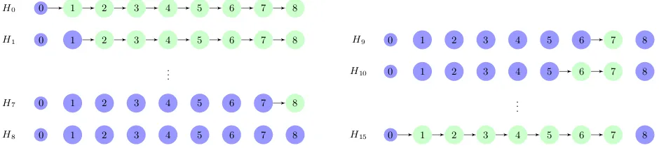
It will be convenient to require that 0 is always contained in S (which makes sense as K0 is always random). In Figure 4 we illustrate the evaluation ofSCG{0,4,5,8}(8). Note that
SCG{0}(N)∼SCG(N, Uλ) and SCG{0,...,N}(N)∼UN λ .
Definition 10. SCG:N× {0,1}λ→ {0,1}∗ is (N, 0, s0)-pseudorandomif no circuit of size s0 can
dis-tinguish with advantage greater than0 the firstN blocks of output ofSCG from random when instantiated with a random key, i.e.,
SCG(N, Uλ)∼(0,s0)UN λ .
We say that SCG is (N, 0, s0) next-block pseudorandom if, for any N0 ≤N, no circuit of size s0 can distinguish the N0-th output block from random given the first N0−1 blocks, i.e.,
SCG(N0, Uλ)∼(0,s0)SCG{0,N0}(N0)∼SCG(N0−1, Uλ)kUλ .
To prove (next-block) pseudorandomness of SCG, we will use a hybrid argument. We call two hybrids
SCGS(N) and SCGS0(N)neighboring ifS andS0 are 1-neighboring, as in Definition 6. The following lemma
shows that two neighboring hybrids are indistinguishable if Gis pseudorandom.
Lemma 4. For anyN ∈N+ and two neighboring setsS ⊂ S0⊆[N]
G(Uλ)∼(,s)U2λ ⇒ SCGS(N)∼(,s0)SCGS0(N) ,
Proof. We assume w.l.o.g. that |S0|>|S|. Given a PRG challengeC∈ {0,1}2λ, we can sample a variable
X s.t.
X∼SCGS(N) if C ∼G(Uλ) and X ∼SCGS0(N) if C∼U2λ
as follows. Let d∈ S0 be the (unique) element not in S. Now sample SCGS(N) as in (16), except that in thed-th step we use (Kd, Xd) :=C. (Note that (Kd−1, Xd−1) is random as per 2. in Definition 6.) Thus, from any distinguisher for SCGS(N) and SCGS0(N), we get a distinguisher for the PRG G with the same
advantage. ut
We will also use the triangle inequality for indistinguishability.
Proposition 4. Consider any random variablesH0, H1, . . . , HN then
H0 6∼(,s)HN ⇒ ∃i∈[N] : Hi−16∼(N,s)Hi .
Together with Lemma 4, this yields that the construction of the stream-cipher SCG in eq. (15) is secure.
Proposition 5. If G: {0,1}λ → {0,1}2λ is an (, s)-secure PRG, then SCG is (N, 0, s0) pseudorandom
with
0 =·N and s0 ≈s−N|G| .
Proof. Consider the hybrids H0, . . . , HN whereHi =SCG[i]0(N) (as illustrated in Figure 5 for N = 8; the
hybrids H9, . . . , H15 in the figure are not needed in this proof). Assume for contradiction that SCG{0}(N)
is not (N, s0) indistinguishable fromSCG[N]
0(N), i.e.,
H0 6∼(N,s0)HN .
Then by Proposition 4, for some i∈[N]
Hi−1 6∼(,s0)Hi .
Since [i−1]0 and [i]0 are neighboring sets, applying Lemma 4, we get,
G(Uλ)6∼(,s0+N|G|)U2λ ,
contradicting (, s)-security ofG. ut
Proposition 6. If G:{0,1}λ → {0,1}2λ is an (, s)-secure PRG, then SCG is (N, 0, s0) next-block
pseudorandom with
0=· 1
2N−1 and s
0 ≈s−(2N−1)|G| .
We omit the proof as it is almost identical to the proof of Proposition 5, except that we use hybridsH0 toH2N−1 (not just HN) as illustrated in Figure 5.
Here each hybrid Hi corresponds to the variable SCGSi(N), for S0, . . . ,S2N−1 ⊆ [N] where S0 =
{0},S2N−1 ={0, N}and for any i, the setsSi−1 and Si are neighboring. Concretely,
S0={0}
Si={0,1, . . . , i} fori∈ {1, . . . , N} (17)
0 1 2 3 4 5 6 7 8
0 1 2 3 4 5 6 7 8
0 1 2 3 4 5 6 7 8
0 1 2 3 4 5 6 7 8
0 1 2 3 4 5 6 7 8
0 1 2 3 4 5 6 7 8
0 1 2 3 4 5 6 7 8
. . .
. . . H0
H1
H7
H8
H9
H10
H15
Fig. 5. The hybrids H0, . . . , HN (for N = 8) are as defined in the proof of Proposition 5. The proof of Proposition 6 additionally uses the hybridsHN+1, . . . , H2N−1.
B Omitted Proofs
B.1 Proof of Lemma 1
From any adversary Af against the full security of F we can construct an adversary As (of basically the same size) against the selective security ofF losing a factor of |X |in the advantage, i.e.
AdvselF (As, q) = |X |1 ·AdvfullF (Af, q) , (18)
as follows. As initially simply outputs a random x0
∗
← X in the selective security game. Using its own oracle to answer Af’s queries, As then runsA
O(·)
f , which outputs somex
∗. If x∗ =x0 then A
s uses Af for the rest of the experiment, i.e., it forwards the challenge Cb to Af and then returns the bit ˜b that Af outputs. Ifx∗ 6=x0 thenAsanswers with ˜b= 0. Thus, As outputs 0 with probability 1−|X |1 , and whatever
Af outputs otherwise. Let (possibly negative) be such that
Prb←{∗
0,1}
ExpfullCPRF(Af,F, b, q) =b] = 12 + . (19)
Then
Pr
b←{∗ 0,1}
[ExpselCPRF(As,F, b, q) =b
= Pr
b←{∗ 0,1}
ExpselCPRF(As,F, b, q) =b
x∗ =x0
Pr[x∗ =x0] +
Pr
b←{∗ 0,1}
ExpselCPRF(As,F, b, q) =b
x∗ 6=x0
Pr[x∗ 6=x0]
= Prb←{∗
0,1}[ExpfullCPRF(Af,F, b, q) =b]·|X |1 +12 · 1− 1
|X |
= 12+|X |1 +12 · 1− 1
|X |
= 12 +|X | .
By (1) this means 2|| 1
|X | =AdvselF (As, q); on the other hand (1) and (19) give 2||=AdvfullF (Af, q), which proves (18).
B.2 Proof of Proposition 2
We consider two hybrid games H0 and Hm, which will correspond to the experiments
H0 ∼AF(K,·) and Hm∼Af(·) , where K
∗
ExperimentHi ∀x∈ {0,1}≤N
: Kx:=⊥
K∅← {0∗ ,1}λ
x∗←As
// Below,Ascan make max.q queries
// and last query must bex∗:
AOs(·)
˜b←A
s
Return ˜b
O(x=x[1. . . `])
// ReturnKxif it is already defined: IfKx6=⊥then returnKx
// Get parent ofKxrecursively
Kx[1...`−1]:=O(x[1. . . `−1])
// ComputeKx and its sibling usingG,
// unlessx[1. . . `−1] is a prefix ofx∗and|x| ∈ Si, // in which case use random values:
Ifx[1. . . `−1] =x∗[1. . . `−1] and`∈ Si then
Kx[1...`−1]k0kKx[1...`−1]k1 ∗ ←U2λ else
Kx[1...`−1]k0kKx[1...`−1]k1 :=G(Kx[1...`−1])
ReturnKx
Fig. 6.Definition of the hybrid gamesH0, . . . , H2N−1 from the proof of Proposition 3, whereSi are as in eq. (17).
For ease of describing the subsequent hybrids, we describe H0 as follows. In H0 we begin by initially defining Kx =⊥ for all x ∈ {0,1}∗ and then sampling K∅
∗
← K. We then invoke A, who makes queries x1, x2, . . . (of total length at most m), where we answer each query x = x[1. . . `] with Kx, defined
as follows: determine the largest `0 s.t. Kx[1...`0] 6= ⊥, and then for j = `0, . . . , `−1 recursively define
Kx[1...jk0]kKx[1...jk1] := G(Kx[1...j]). The output of H0 is whatever A finally outputs. We just emulated
F(K,·) for A, and thus H0 ∼AF(K,·).
Now for any i≥0, we define the experimentHi to be the same as the experiment H0, except that we replace the outputs of the firstiinvocations ofGwith uniformly random values. We haveHm ∼Af(·), as
all the outputsAgets in Hm are uniformly random, exactly like the outputs of f(·).
It follows that ifAcan distinguishF(K,·) from a random function (i.e., distinguishH0 fromHm) with
advantagethen there are two hybrids Hi, Hi+1 s.t.
Pr[1←Hi]−Pr[1←Hi+1] ≥ m .
Using this, we can distinguish the output G(Uλ) from a random U2λ with the same advantage: given a
challengeC, simulate the experimentHi up to the (i+ 1)-th invocation ofG, and replace its output with
C. IfC =G(Uλ), this emulates experimentHi, and if C =U2λ, this emulates experimentHi+1.
B.3 Proof of Proposition 3
Full security as stated in Item2. of the proposition follows from selective security (Item1.) by complexity leveraging as explained in Lemma 1.
To prove selective security, we will use hybrid gamesH0, . . . , H2N−1 as defined in Figure 6. By inspec-tion we see that the first and last hybrids defined in Figure 6 are exactly the real and random selective security game, i.e.,
H0 ∼ExpselCPRF(As,GGMG,0, q) and H2N−1 ∼ExpselCPRF(As,GGMG,1, q) .
The other hybrids correspond to games where we sometimes use uniformly random values instead of the output of G on the path from the root K∅ to the challenge output Kx∗. More precisely, in Hi we use
random values in the j-th step along the path computing the output for x∗ for all j ∈ Si, with Si as in