Efficient Template Attacks
Omar Choudary and Markus G. Kuhn
Computer Laboratory, University of Cambridge [email protected]
Abstract. Template attacks remain a powerful side-channel technique to eavesdrop on tamper-resistant hardware. They model the probabil-ity distribution of leaking signals and noise to guide a search for se-cret data values. In practice, several numerical obstacles can arise when implementing such attacks with multivariate normal distributions. We propose efficient methods to avoid these. We also demonstrate how to achieve significant performance improvements, both in terms of informa-tion extracted and computainforma-tional cost, by pooling covariance estimates across all data values. We provide a detailed and systematic overview of many different options for implementing such attacks. Our experimental evaluation of all these methods based on measuring the supply current of a byte-load instruction executed in an unprotected 8-bit microcontroller leads to practical guidance for choosing an attack algorithm.
Keywords:side-channel attacks, template attack, multivariate analysis.
1
Introduction
Side-channel attacks are powerful tools for inferring secret algorithms or data (passwords, cryptographic keys, etc.) processed inside tamper-resistant hard-ware, if an attacker can monitor some channel leaking such information out of the device, most notably the power-supply current and unintended electromag-netic emissions.
One of the most powerful techniques for evaluating side-channel information is thetemplate attack[4], which relies on a multivariate model of the side-channel traces. While the basic algorithm is comparatively simple (Section 2), there are a number of additional steps that must be performed in order to obtain a practical and efficient implementation.
We evaluate all these methods in practice, against an unprotected 8-bit mi-crocontroller, comparing their effectiveness using the guessing entropy (Section 6). We focus on gathering information about individual data values,independent
of what algorithm these are part of. Other algorithm-specific attacks that use dependencies between different data values, e.g. to recover keys from a specific cipher, could be implemented on top of that, but are outside the scope of this paper. We show that PCA and LDA provide the best results overall, and that a previous guideline of selecting at most one point per clock cycle is not optimal in general. Based on these experiments and theoretical background, we provide practical guidance for the choice of template-attack algorithm.
2
Template Attacks
To implement a template attack, we need physical access to a pair of identical devices, which we refer to as theprofiling and theattacked device. We wish to infer some secret valuek?∈ S, processed by the attacked device at some point. For an 8-bit microcontroller, S={0, . . . ,255} might be the set of possible byte values manipulated by a particular machine instruction.
We assume that we determined the approximate moments of time when the secret value k? is manipulated and we are able to record signal traces (e.g., supply current or electro-magnetic waveforms) around these moments. We refer to these traces as leakage vectors. Let{t1, . . . , tmr} be the set of timesamples andxr∈
Rm r
be the random vector from which leakage traces are drawn. During theprofiling phase we record npleakage vectorsxrki∈R
mr
from the profiling device for each possible valuek∈ S, and combine these as row vectors
xr
ki
0 in the leakage matrixXr
k∈R np×mr.1
Typically, therawleakage vectorsxr
kiprovided by the data acquisition device
contain a large numbermrof samples (random variables), due to high sampling
rates used. Therefore, we mightcompress them before further processing, either by selecting only a subset of m mr of those samples, or by applying some
other data-dimensionality reduction method (see Section 4). We refer to such compressed leakage vectors as xki ∈Rm and combine all of these as rows into the compressed leakage matrix Xk ∈ Rnp×m. (Without any such compression step, we would haveXk=Xrk andm=mr.)
Using Xk we can compute the template parameters ¯xk ∈ Rm and Sk ∈ Rm×m for each possible valuek∈ S as
¯
xk= n1 p
np
X
i=1
xki, Sk= n1
p−1
np
X
i=1
(xki−¯xk)(xki−¯xk)0, (1)
where the sample mean ¯xk and the sample unbiased2 covariance matrixSk are
the estimates of the true mean µk and true covarianceΣk. Note that a sum of
1 Throughout this paperx0
is the transpose ofx. 2
squares and cross products matrix such as
np
X
i=1
(xki−xk¯ )(xki−xk¯ )0,from (1) can
also be written as
np
X
i=1
(xki−x¯k)(xki−x¯k)
0
=Xe0kXek, (2)
whereXek isXk with ¯x0k subtracted from each row.
3
Side-channel leakage traces can generally be modeled well by a multivariate normal distribution [4], which we also observed in our experiments. In this case, the sample mean ¯xk and sample covarianceSkaresufficient statistics: they com-pletely define the underlying distribution [10, Chapter 4]. Then the probability density function (pdf) of a leakage vectorx, given ¯xk and Sk, is
f(x|xk¯ ,Sk) = p 1
(2π)m|Sk|exp
−1
2(x−xk¯ )
0
S−k1(x−¯xk)
. (3)
In the attack phase, we try to infer the secret value k? ∈ S processed by the attacked device. We obtain na leakage vectors xi ∈Rm from the attacked device, using the same recording technique and compression method as in the profiling phase, resulting in the leakage matrix Xk? ∈ Rna×m. Then, for each
k∈ S, we compute adiscriminant score d(k|Xk?). Finally, we try allk∈ S on the attacked device, in order of decreasing score (optimized brute-force search, e.g. for a password or cryptographic key), until we find the correctk?. Given a tracexi fromXk?, a commonly used discriminant [8,11,14], derived from Bayes’ rule, is
d(k|xi) = f(xi|¯xk,Sk)P(k), (4)
where the denominator from Bayes’ rule is omitted, as it is the same for each
k. Assuming a uniform a-priori probability P(k) = |S|−1, applying Bayes’ rule
becomes equivalent to computing the likelihood
l(k|xi) = d(k|xi) = l(¯xk,Sk |xi) = f(xi|¯xk,Sk), (5)
where the latter can be computed from (3). However, we do not need to compute a proper a-posteriori probability for each candidatekgiven a tracexi, but only a discriminant function that allows us to sort scores and identify the most likely candidates. Section 5 shows how the latter can be much more efficient.
3
Implementation Caveats
We now present several problems that can appear when implementing the tem-plate attack, especially when using a large number of samplesm.
Σkis theunbiased estimatorwith 1/(np−1); the MLE merely maximises the joint likelihood from the multivariate normal distribution. In practice, we found this choice made no significant performance difference (even down tonp= 10, m= 6). 3
3.1 Inverse of Covariance Matrix
Several authors [15,14] noted that inverting the covariance matrixSk from (1),
as needed in (3), can cause numerical problems for largem. However, we consider it important to explain why Sk can become singular (|Sk| ≈ 0), causing these
problems.
SinceSk is essentially the matrix productXe0kXek (2), bothSk and Xek have
the same rank. ThereforeSk is singular iffXke has dependent columns, which is
guaranteed ifnp< m. The constraint onXke to have zero-mean rows implies that
it has dependent columns even for np =m. Therefore, np > m is a necessary
condition forSkto be non-singular. See [10, Result 3.3] for a more detailed proof.
The restrictionm < npis one main reason for reducingm through
compres-sion (see Section 4). However, it is not mandatory to compressm further than what is needed to keep the columns of Xke independent. Note that in practice
some samples can be highly correlated, in which casenpneeds to be somewhat
larger thanm (e.g., np≥3000 form= 1250 with our Section 6 data).
If we cannot obtain np > m then we can try the covariance estimator of
Ledoit and Wolf [5], which gave us a non-singularSkeven fornp< m. However,
a much better option is to use the pooled covariance matrix (see Section 5.2) when possible.
3.2 Floating-point Limitations
One practical problem with (3) is that for largem the statistical distance
(x−xk¯ )0Sk−1(x−¯xk)
can reach values that cause the subsequent exponentiation operation to overflow. For example, in IEEE double precision, exp(x) is only safe with|x|<710, easily exceeded for largem.
Another problem is that for largem the determinant |Sk|can overflow. For
example, considering that |Sk|is the product of the eigenvalues of Sk, in some
of our experiments the 100 largest eigenvalues were at least 106 and multiplying
merely 52 such values again overflows the IEEE double precision format.
4
Compression Methods
A compression method can be used to reduce the length (dimensionality) of leakage vectors from mr tom. As detailed in Section 3, this may be needed if
we do not have enough traces for a full rank covariance matrix or to cope with computational or memory restrictions. Several approaches are described in the literature, which can be divided into two categories: (a) selecting some of the samples based on some criteria; (b) using some linear combinations of the leakage vectors, based on the principal components or Fisher’s linear discriminant. All of the following techniques evaluate the differences ¯xk−x¯ where
¯
x= 1
|S| X
k∈S
¯
1 1.5 2 2.5 clock cycles
dom sosd snr std clock
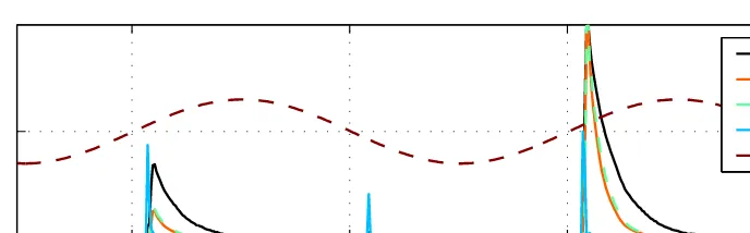
Fig. 1. Signal-strength estimates from DOM, SOSD and SNR (identical to SOST) for a LOAD instruction processing all possible 8-bit values, along with the average standard deviation (STD) of the traces and clock signal. We used 2000 traces per value. All estimates are rescaled to fit into the plot, so the vertical axis (linear) has no scale.
4.1 Selection of Samples
In this method we first compute a signal-strength estimates(t), t∈ {t1, . . . , tmr}, and then we select a subset ofm points based on this estimate.
There are several proposals for producings(t), such as difference of means (DOM) [4, Section 2.1], thesum of squared differences (SOSD) [9], theSignal to Noise Ratio (SNR)[15] andSOST [9]. All these are similar, with the notable difference that the first two do no take the variance of the traces into considera-tion, while the latter two do. We show the difference between these estimates for our experiments in Figure 1. The methods SNR and SOST are in fact the same if we consider the variance at each sample point to be independent of the can-didatek, which is expected in our setting. Under this condition SNR and SOST reduce to computing the following value used by the F-test in the Analysis of Variance [10]:
F(t) =
np
X
k∈S
(¯xk(t)−x¯(t))2 !
(|S| −1)
X
k∈S
np
X
i=1
(xki(t)−¯xk(t))2
!
(|S|(np−1))
. (7)
F(t) can be used to reject, at any desired significance level, the hypothesis that the sample mean values at sample pointtare equal, therefore providing a good indication of which samples contain more information about the means.
4.2 Principal Component Analysis (PCA)
Archambeau et al. [8] proposed the following method for using PCA as a com-pression method for template attacks. First compute thesample between groups
matrixB:
B=np
X
k∈S
(¯xrk−x¯r)(¯xrk−x¯r)0. (8)
Next obtain the singular value decomposition (SVD) B =UDU0, where each column of U ∈Rmr×mr is an eigenvector u
j of B, and D ∈ Rm r×mr
contains the corresponding eigenvaluesδj on its diagonal.4The crucial point is that only
the firstm eigenvectors [u1. . .um] =Umare needed in order to preserve most
of the information from the mean vectors ¯xr
k. Therefore we can restrict U to Um ∈
Rm r×m
. Finally, we can project the mean vectors ¯xr
k and covariance
matricesSr
k (computed with (1) on the raw tracesxri) into the new coordinate
system defined by Um to obtain the PCA template parameters ¯xk ∈ Rm and
Sk∈Rm×m:
¯
xk=Um0x¯r
k, Sk=Um
0Sr
kUm. (9)
Choice of PCA Components. Archambeau et al. [8] propose to select only those first m eigenvectorsuj for which the corresponding eigenvalues δj are a
few orders of magnitude larger than the rest. This technique, also known as
elbow rule or Scree Graph [6], requires manual inspection of the eigenvalues. Another technique, which does not require manual inspection of the eigenvalues, is known as theCumulative Percentage of Total Variation [6]. It selects thosem
eigenvectors that retain at least fraction f of the total variance, by computing the score
φ(m) =
P
1≤j≤mδj P
1≤j≤mrδj
, 1≤m ≤mr, (10)
and selecting the lowest m for which φ(m)> f.5 We recommend trying both
approaches, as “there is no definitive answer [to the question of how many com-ponents to choose]” [10, Chapter 8].
Alternative Computation of PCA Templates. Even though in [11, Section 4.1] the authors mention that PCA can help where computing the full covariance matrix Sr
k is prohibitive (due to large m
r), their approach still requires the
computation ofSr
k (see (9)). Also, numerical artifacts during the double matrix
4
Archambeau et al. [8] show a method for computingUthat is more efficient when mr |S|, but in our experiments withmr= 2500 this direct approach worked well. 5
multiplication in (9) can makeSk non-symmetric. One way to avoid the latter
is to use the Cholesky decompositionSr
k =C
0Cand compute
Sk =Um0SrkUm=Um0C0CUm= (CUm)0(CUm) =V0V. (11)
However, to avoid both the numerical artifacts and the computation of large covariance matrices, we propose an alternative PCA method, based on the fol-lowing result: given the leakage matrixXr
k and the PCA projection matrixUm,
it can be shown [10, Eq. (2-45)] that
Sk= Cov(XrkU
m) =Um0Cov(Xr
k)U
m=Um0Sr
kU
m. (12)
Therefore, instead of first computingSr
k and then applying (9) or (11), we
can first compute the projected leakage matrix
Xk=XrkU
m (13)
and then compute the PCA-based template parameters using (1). We use this method for all the results shown in Section 6.
4.3 Fisher’s Linear Discriminant Analysis (LDA)
Given the leakage tracesxr
ki (rows ofXrk), Fisher’s idea [2,10] was to find some
coefficientsaj ∈Rm r
that maximise the following ratio:
X
k∈S
(¯ykj−y¯j)2
Var(yj)
=
X
k∈S
(aj0(¯xrk−x¯r))2
Var(aj0x)
= aj
0Baj
aj0Spooledaj
, (14)
where the linear combinations yj = aj0x are known as sample discriminants, B is the treatment matrix from (8) and Spooled = |S|1 Pk∈SS
r
k is the common
covariance of all groups (see also Section 5.2). Note the similarity between the left hand side of (14) and (7) which is used by the F-test, SNR and SOST. This allows us to make an interesting observation: while in the sample selection method we first compute (7) for each sample and then select the samples with the highest F(t), Fisher’s method finds the linear combinations of the trace samples that maximise (14). The coefficientsaj that maximise (14) are the eigenvectors [u1. . .umr] =Ucorresponding to the largest eigenvalues ofS−pooled1 B.6
As with PCA, we only need to use the firstm coefficientsa1, . . . ,am, which
can be selected using the same rules discussed in Section 4.2. If we let A = [a1. . .am] = Um be the matrix of coefficients, we can project each leakage
matrix as:
Xk =XrkA=X
r
kU
m (15)
and compute the LDA-based template parameters using (1).
6
Several authors [11,14] have used Fisher’s LDA for template attacks, but without mentioning two important aspects. Firstly, the condition of equal covari-ances (known ashomoscedasticity) may be important for the success of Fisher’s LDA. Therefore, the PCA method (Section 4.2), which does not depend on this condition, might be a better choice in some settings. Secondly, the coefficients that maximise (14) can be obtained using scaled versions ofSpooled7or different
approaches [11,14], which will result in a different scale of the coefficientsaj. This difference has a major impact on the template attack: only when we scale the coefficientsaj, such thataj0Spooledaj = 1, the covariance between discriminants
becomes the identity matrix [10], i.e.Sk =I. That means the sample means in (1) suffice and we can discard the covariance matrix from the discriminant scores in Section 5, which greatly reduces computation and storage requirements.
Continuing the steps that led to (15), we can compute the diagonal matrix
Q ∈ Rm×m, having the values qjj = (aj0S 1 pooledaj)
1
2 = ( 1
uj0Spooleduj) 1 2 on its diagonal, to obtain the scaled coefficientsAQ=UmQ, and replace (15) by
Xk=XrkAQ=X
r
kU
mQ. (16)
An alternative approach is to compute the eigenvectorsujofS
−1 2
pooledBS
−1 2
pooledand
then obtain the coefficients aj =S−
1 2
pooleduj, which leads directly to coefficients
that satisfyaj0Spooledaj = 1.
5
Efficient Implementation of Template Attacks
In this section we introduce methods that avoid the problems identified in Sec-tion 3 and implement template attacks very efficiently.
5.1 Using the Logarithm of the Multivariate Normal Distribution
Mangard et al. [15, p. 108] suggested calculating the logarithm of (3), as in
log f(x|¯xk,Sk) =−1
2 log [(2π)
m|Sk|] + (x−xk¯ )0
S−k1(x−xk¯ ). (17)
They then claim that“the template that leads to the smallest absolute value [of (17)] indicates the correct [candidate]”.
The first problem with this approach is that (17) does not avoid the compu-tation of|Sk|, which we have shown to be problematic. Therefore we propose to compute the logarithm of the multivariate normal pdf as
log f(x|x¯k,Sk) =−
m
2 log 2π− 1
2log|Sk| − 1
2(x−x¯k)
0
S−k1(x−x¯k), (18)
7
Instead ofSpooledwe could useW=|S|(np−1)Spooled, known as asample within
where we compute the logarithm of the determinant as
log|Sk|= 2 X
cii∈diag(C)
logcii, (19)
using the Cholesky decompositionSk =C0Cof the symmetric matrixSk. (Since
C is triangular, its determinant is the product of its diagonal elements.) Secondly, it is incorrect to choose the candidatekthat leads to the “small-est absolute value” of (17,18), since the logarithm is a monotonic function and preserves the property that thelargest value corresponds to the correctk.8
We can use (18,19), dropping the first term which is constant across allk, to compute a discriminant score based on the log-likelihood:
dLOG(k|xi) =−
1
2log|Sk| − 1
2(xi−xk¯ )
0
S−k1(xi−xk¯ ) (20)
= log f(xi |xk¯ ,Sk) +m
2 log 2π= log l(k|xi) + const.
5.2 Using a Pooled Covariance Matrix
When the leakages from different candidates k have different means but the same covarianceΣ =Σ1=Σ2=· · ·=Σk, it is possible topool the covariance
estimatesSk into apooledcovariance matrix [10, Section 6.3]
Spooled=
1
|S|(np−1)
X
k∈S
np
X
i=1
(xki−x¯k)(xki−x¯k)
0
, (21)
an average of the covariancesSk from (1). The great advantage of Spooled over
Sk is that it represents a much better estimator of the real covariance Σ, since
Spooled estimates the covariance usingnp|S|traces, whileSk uses onlynp. This
in turn means that the condition for a non-singular matrix (see Section 3.1) relaxes tonp|S|> m ornp> |S|m. Therefore the number of traces that we must
obtain for each candidate k is reduced by a factor of|S|, a great advantage in practice. Nevertheless, the quality of the mean estimate ¯xk still depends directly
on np. Also note that for Fisher’s LDA (Section 4.3) we need to compute the
inverse ofSpooled ∈Rm r×mr
, which requiresnp|S|> mr.
Several authors usedSpooled with template attacks [12,16], but gave no
moti-vation for its use. We would expect the assumption of equal covariances to hold for many side-channel applications, because Sk captures primarily information about hownoise, that is variation in the recorded traces unrelated tok, is corre-lated across trace samples. After all, the data-dependent signal ¯xk was already
subtracted. As a result, we should not expect substantial differences between the Sk for different candidate values k, unless the targeted device contains a
8
mechanism by which k can modify the correlation between samples (which we do not completely exclude).
Box’s test [3] can be used to reject the hypothesis of equal covariances, al-though it can be misleading for large |S| or largem. In our experiments, with
|S| = 28, m = 6 and n
p = 2000, Box’s variable C ∼Ff1,f2(α) had the value
2.03, which was above the rejection threshold for any realistic significance level (e.g. Ff1,f2(0.99) = 1.045). Nevertheless, we found the differentSk to be
visu-ally similar (viewed as bitmaps with linear colour mapping), and we consider that our hypothesis was confirmed by the superior results from using the pooled estimate (Section 6).
UsingSpooled, we can discard the first two terms in (18) and use the
gener-alized statistical distance
d2M(x|xk¯ ,Spooled) = (x−xk¯ )0S−pooled1 (x−xk¯ )≥0, (22)
also known as the Mahalanobis distance [1], to compare the candidatesk. The inequality in (22) holds because the covariance matrix is positive semidefinite. From (18,22) we can derive the discriminant score
dMD(k|xi) =−
1 2d
2
M(xi|x¯k,Spooled) = dLOG(k|xi) + const., (23)
where the constant does not vary withk.
5.3 Linear Discriminant Score
When using the pooled covariance matrix Spooled we can rewrite the distance
from (22) as:
d2M(x|¯xk,Spooled) =x0S−pooled1 x−2¯x 0
kS−
1
pooledx+ ¯x
0
kS−
1
pooled¯xk, (24)
and observe that the first term is constant for all groupskso we can discard it. That means, that we can now use the followinglinear discriminant score:
dLINEAR(k|xi) = ¯x0kS−
1
pooledxi−
1 2¯x
0
kS−
1
pooled¯xk= dMD(k|xi) + const., (25)
which depends linearly on xi (where const. does not depend on k). Although equivalent, the linear discriminant dLINEAR can be far more efficient to compute
than the quadratic dMD.
5.4 Combining Multiple Attack Traces
We have to combine thena individual leakage tracesxi fromXk? into the final
Option 1: Average all the traces inXk? (similar to the mean computation in
(1)) in order to remove as much noise as possible and then use this single mean trace ¯xk?to compute
davg(k|Xk?) = d(k|¯xk?). (26)
This option is computationally fast, requiringO(nam+m2) time for any
pre-sented discriminant, but it does not use all the information from the available attack traces (in particular the noise).
Option 2: Compute the joint likelihood l(k | Xk?) = Y
xi∈Xk?
l(k | xi). By
applying the logarithm to both sides we have log l(k|Xk?) = X
xi∈Xk?
log l(k|xi)
and we obtain the derived scores:
djointLOG(k|Xk?) =−na
2 log|Sk| − 1 2
X
xi∈Xk?
(xi−xk¯ )0Sk−1(xi−¯xk), (27)
djointMD(k|Xk?) =−1
2
X
xi∈Xk?
(xi−xk¯ )0Sk−1(xi−¯xk), (28)
djointLINEAR(k|Xk?) = ¯x0kS−
1 pooled
X
xi∈Xk?
xi
−na
2 x¯
0
kS−
1
pooledx¯k. (29)
Given thenaleakage tracesxi∈Xk?, dLOGand dMDrequire timeO(nam2)
while dLINEAR only requires O(nam+m2), since the operations ¯x0kS
−1
pooled and
¯
x0kS−pooled1 xk¯ only need to be done once, which is a great advantage in practice.
As a practical example, our evaluations of the guessing entropy (see Section 6) for m = 125 and 1≤ na ≤ 1000 took about 3.5 days with dLOG but only 30
minutes with dLINEAR.9We note that for dLINEARthe computation time is the
same regardless of which option we use to combine the traces, and both give the same results for the template attack.
5.5 Unequal Prior Probabilities
In the previous descriptions we have assumed equal prior probabilities among the candidatesk. When this is not the case, we only need to add the term logP(k) to the discriminant scores davgLOG, davgMD, dLINEARavg , ornalogP(k) to the discriminant
scores djointLOG, djointMD, djointLINEAR.
6
Evaluation of Methods
We evaluated the efficiency of many template-attack variants on a real hard-ware platform, comparing all the compression methods from Table 110 and all
9
MATLAB, single core CPU with 3794 MIPS.
10We arbitrarily chose to use the DOM estimate, computed as the sum of absolute
Table 1.List of compression methods evaluated in this paper.
Name Description m
DOM 1ppc DOM, 1 sample per clock at most 6–10
DOM 3ppc DOM, 3 samples per clock at most 18–30
DOM 20ppc DOM, 20 samples per clock at most 75–79
DOM allap DOM, all samples above 95th percentile of F(t) 125
PCA Fixed selection of number of principal components 4
LDA Fixed selection of number of coefficients 4
the implementation options from Section 5. We compare the commonly used high-compression methods, such as PCA, LDA and sample selection using the guideline [7] of 1 sample per clock at most (1ppc), against weak compressions providing a larger number of samples: the 3ppc,20ppcandallap selections.11
6.1 Experimental Setup
Our target is the 8-bit CPU Atmel XMEGA 256 A3U, an easily available micro-controller without side-channel countermeasures, mounted on our own evaluation board to monitor the total current in all CPU ground pins via a 10 ohm resistor. We powered it from a battery via a 3.3 V regulator and supplied a 1 MHz sine clock. We used a Tektronix TDS 7054 8-bit oscilloscope with P6243 active probe, at 250 MS/s, with 500 MHz bandwidth in SAMPLE mode. We used the same device for both the profiling and the attack phase, which provides a good setting for the focus of our work.
For each candidate valuek∈ {0, . . . ,255} we recorded 3072 tracesxrki (i.e., 786 432 traces in total), which we divided into a training set (for the profil-ing phase) and an evaluation set (for the attack phase). Each trace contains
mr= 2500 samples, recorded while the target microcontroller executed the same sequence of instructions loaded from the same addresses: a MOV instruction, followed by several LOAD instructions. All the LOAD instructions require two clock cycles to transfer a value from RAM into a register, using indirect address-ing. In all the experiments our goal was to determine the success of the template attacks in recovering the byte k processed by the second LOAD instruction. All the other instructions were processing the value zero, meaning that in our traces none of the variability should be caused by variable data in other nearby instructions that may be processed concurrently in various pipeline stages.12
11The selections 1ppc, 3ppc and 20ppc provide a variable number of samples because
of the additional restriction that the selected samples must be above the highest 95th percentile of F(t), which varies withnpfor each clock edge.
12
6.2 Guessing Entropy
We use theguessing entropy as the sole figure of merit to compare all methods. It estimates the (logarithmic) cost of any optimized search following a template attack to find the correctk?among the values kwith the highest discriminant scores. It gives the expected number of bits of uncertainty remaining about the target valuek?. The lower the guessing entropy, the more successful the attack has been and the less effort remains to search for the correctk?.
To compute the guessing entropy, we compute the score d(k|Xk?) (see Sec-tion 5) for each combinaSec-tion of candidate valuekand target value k?, resulting in a score matrix M ∈ R|S|×|S| with M(k?, k) = d(k | Xk?). Each row in M contains the score of each candidate valuekgiven the tracesXk?corresponding to a given target valuek?. Next we sort each row ofM, in decreasing order, to obtain a depth matrixD∈N|S|×|S| with
D(k?, k) = position of d(k|Xk?) in the sorted row ofM(k?,·). (30)
Finally, using the matrixD we define the guessing entropy
g= log2 1
|S| X
k∈S
D(k, k). (31)
Standaert et al. [13] also used this measure, but without the logarithm.
6.3 Experimental Results and Practical Guidance
We performed each attack 10 times for each combination ofna,kandk?, using
a different random selection of Xk? for each na and k?. We plot in Figure 2
and 3 the averaged guessing entropy, resulting in highly reproducible graphs. The standard deviation across all experiments is around 0.1 bits.
These results, as well as the considerations discussed earlier, allow us to provide the following practical guidance regarding the choice of algorithm:
1. Use Option 2 (djoint) in preference to Option 1 (davg) to combine the
dis-criminant scores forna>1 attack traces.Forna= 1 or when usingSpooled,
these options are equivalent. Otherwise, as the numberna of attack traces
increases and the covariance matrix is better estimated (e.g. due to a large numbernpof profiling traces or small numberm of variables) djoint
outper-forms davg for all compression methods.
2. Try using a common covariance matrix Spooled with dLINEAR (unless
dif-ferences between individual estimatesSk are very evident, e.g. from visual inspection). Failing a statistical test for homoscedasticity (e.g., Box’s test) alone does not imply that using individual estimates Sk will improve the
template attack. Using individual estimates Sk prevents use of the
signifi-cantly faster and more robust discriminant dLINEAR. Then:
(a) If your target allows you to acquire a large number of traces (na>100):
try the compression methods PCA, LDA and sample-selection withlarge
100 101 102 103 0
1 2 3 4 5 6
na(log axis)
Guessing entropy (bits)
100 101 102 103 0
1 2 3 4 5 6
na(log axis)
Guessing entropy (bits)
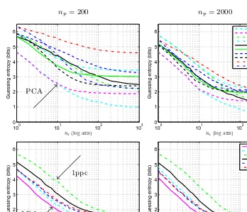
PCA, m=4 joint PCA, m=4 avg sample, 1ppc joint sample, 1ppc avg sample, 3ppc joint sample, 3ppc avg sample, 20ppc joint sample, 20ppc avg sample, allap joint sample, allap avg
100 101 102 103 0
1 2 3 4 5 6
na(log axis)
Guessing entropy (bits)
100 101 102 103 0
1 2 3 4 5 6
na(log axis)
Guessing entropy (bits)
LDA, m=4 PCA, m=4 sample, 1ppc sample, 3ppc sample, 20ppc sample, allap
Sk
(d
LOG
)
Sp
o
oled
(d
LINEAR
)
np= 200 np= 2000
PCA
LDA
1ppc
Fig. 2. Guessing entropy remaining after template attacks, with different compres-sions, for np = 200 (left) and np = 2000 (right) profiling traces, using individual covariancesSkwith dLOG(top) or a pooled covarianceSpooledwith dLINEAR(bottom).
(b) If your target allows only acquisition of a limited number of attack traces (na < 10): use LDA. Note that in this case, as the covariance
esti-mate improves due to large |S|np, performance increases with larger
m (cf. 3ppc, 20ppc, allap). In particular, for na < 10, we see in
Fig-ure 2 (bottom) that we got more than 1 bit of data from 20ppc and
allapcompared to1ppc, which contradicts the claim [7, Section 3.2] that “additional [samples] in the same clock cycle do not provide additional information”. In this setting,20ppcandallap can outperform PCA.
3. If you cannot use the pooled covariance Spooled, then use the individual
co-variancesSk withdLOG and use PCA as the compression method.
np na= 1
200 2000
1 2 3 4 5 6
np na= 1000
200 2000
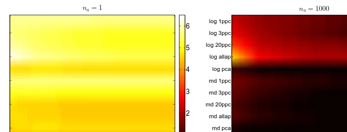
log 1ppc
log 3ppc
log 20ppc
log allap
log pca
md 1ppc
md 3ppc
md 20ppc
md allap
md pca
md lda 1
2 3 4 5 6
Fig. 3. Guessing entropy from the methods discussed, for na = 1 (left) and na = 1000 (right), using djoint (atnp∈ {200,500,1000,1500,2000}, linearly interpolated).
7
Conclusions
In this paper, we have explored in detail the implementation of template attacks based on the multivariate normal distribution, comparing different compression methods, discriminant scores, and number of profiling and attack traces.
We explained why several numerical obstacles arise when dealing with a large number mof variables (e.g. when retaining a large part of the leakage vectors), and we presented efficient methods that can be used in this case, such as the discriminant dLOG.
Based on the observation that the covariance matricesSk of each candidate
kare similar, we explained the use of the pooled covariance estimateSpooled and
we showed howSpooled allows us to derive alinear discriminant dLINEAR which
is much more efficient than dLOG. For na = 1000 attack traces and m = 125
samples, the computation of the guessing entropy remaining after the template attacks can be reduced from 3 days (using dLOG) to 30 minutes (using dLINEAR).
This is a great advantage for the evaluation of template attacks, which is often a requirement to obtain Common Criteria certification.
We applied all the methods presented in this paper on real traces from an unprotected 8-bit microcontroller and we evaluated the results using the guessing entropy. Using the efficient methods presented in this paper we were able to obtain a guessing entropy close to 0, i.e. we are able to extractall8 bits processed by asingle LOAD instruction, not just their Hamming weight.
Based on these results and theoretical arguments, we proposed a practical guideline for the choice of algorithm when implementing template attacks.
Data and Code Availability:In the interest of reproducible research we make available our data and associated MATLAB scripts at:
http://www.cl.cam.ac.uk/research/security/datasets/grizzly/
References
1. P.C. Mahalanobis, “On the Generalised Distance in Statistics”. In: Proceedings National Institute of Science, India, vol. 2, pp 49–55, 1936.
2. R.A. Fisher, “The Statistical Utilization of Multiple Measurements”, in Annals of Eugenics, 8, pp 376–386, 1938.
3. G.E.P. Box, “Problems in the Analysis of Growth and Wear Curves”, in Bio-metrics, 6, pp 362–389, 1950.
4. S. Chari, J. Rao, and P. Rohatgi, “Template Attacks”, CHES 2002, Springer, 2003, LNCS 2523, pp 51–62.
5. O. Ledoit, M. Wolf, “A well-conditioned estimator for large-dimensional covari-ance matrices”, in Journal of Multivariate Analysis, 2004.
6. I. Jolliffe, “Principal Component Analysis”. John Wiley & Sons, Ltd, 2005. 7. C. Rechberger and E. Oswald, “Practical Template Attacks”, in Information
Security Applications, Springer, 2005, LNCS 3325, pp 440–456.
8. C. Archambeau, E. Peeters, F. Standaert, and J. Quisquater, “Template Attacks in Principal Subspaces”, in CHES 2006, Springer, 2006, LNCS 4249, pp 1–14. 9. B. Gierlichs, K. Lemke-Rust, and C. Paar, “Templates vs. Stochastic Methods”,
in CHES 2006, Springer, LNCS 4249, pp 15–29.
10. R. Johnson and D. Wichern, “Applied Multivariate Statistical Analysis”, 6th ed. Pearson, 2007.
11. F.-X. Standaert and C. Archambeau, “Using Subspace-Based Template Attacks to Compare and Combine Power and Electromagnetic Information Leakages”, in CHES 2008, Springer, LNCS 5154, pp 411–425.
12. L. Batina, et al. “Comparative Evaluation of Rank Correlation Based DPA on an AES Prototype Chip”, Information Security, 2008, LNCS 5222, pp 341–354. 13. F.-X. Standaert, et al. “A Unified Framework for the Analysis of Side-Channel
Key Recovery Attacks”, Eurocrypt 2009, LNCS 5479, pp 443–461.
14. T. Eisenbarth, C. Paar, and B. Weghenkel, “Building a Side Channel Based Disassembler”, Trans. on Computational Science X, 2010, vol. 6340, pp 78–99. 15. S. Mangard, E. Oswald, and T. Popp, “Power Analysis Attacks: Revealing the
Secrets of Smart Cards”, 1st ed., Springer, 2010.
16. D. Oswald and C. Paar, “Breaking Mifare DESFire MF3ICD40: Power Analysis and Templates in the Real World”, in CHES 2011, LNCS 6917, pp 207–222.
A
Evaluation Board
For our experiments, we built a custom PCB for the Atmel microcontroller (see Figure 4, left). This 4-layer PCB has inputs for the clock signal and supply voltage, a USB port to communicate with a PC, and a 10-ohm resistor in the ground line for power measurements. The PCB connects all the ground pins of the microcontroller to the same line, which leads to the measurement resistor.
B
Executed Code
5a5c: 00 00 nop ; several previous NOPs ommited in this listing 5a5e: fc 01 movw r30, r24 ; 1 clock cycle, recorded traces start here 5a60: 81 90 ld r8, Z+ ; 2 clock cycles per ld instruction
5a62: 91 90 ld r9, Z+ ; this is our target instruction (2 clock cycles) 5a64: a1 90 ld r10, Z+ ; we want to infer the data loaded in r9 5a66: b1 90 ld r11, Z+
5a68: c1 90 ld r12, Z+ ; recorded trace ends after first clock cycle of this ld
The load instructions use the Z pointer (which refers to registers r31:r30) for indirect RAM addressing. The initial value of registers r8–r12 before the load operations is zero. The initial value of Z before the first load instruction is 2020.
C
Some Proofs
In Section 5.3 we rewrote (22) as (24). This is possible because
¯
x0kS−pooled1 x= (¯x0kS−pooled1 x)0=x0S−pooled1 0x¯k =x0S−pooled1 ¯xk. (32)
In Section 5.4 we state that dLINEAR provides the same results for both
op-tions of combining the traces (from average trace and based on joint likelihood). This happens because if we letck=−12x¯0kS
−1
pooled¯xk for anyk, then we have
djointLINEAR(k|Xk?) = ¯x0kS −1 pooled
X
xi∈Xk?
xi
+nack, (33)
davgLINEAR(k|Xk?) = ¯x 0 kS −1 pooled 1 na X
xi∈Xk?
xi
+ck, (34)
and therefore for anyu, v∈ S it is true that
davgLINEAR(u|Xk?)>davgLINEAR(v|Xk?)⇔
¯
x0uS −1 pooled 1 na X
xi∈Xk?
xi
+cu>x¯0vS −1 pooled 1 na X
xi∈Xk?
xi
+cv⇔
¯
x0uS −1 pooled
X
xi∈Xk?
xi
+nacu>x¯ 0 vS −1 pooled X
xi∈Xk?
xi
+nacv⇔
djointLINEAR(u|Xk?)>djointLINEAR(v|Xk?).
0 2 4 6 8 10
−2 −1 0 1 2 3x 10
4
Time [µs]
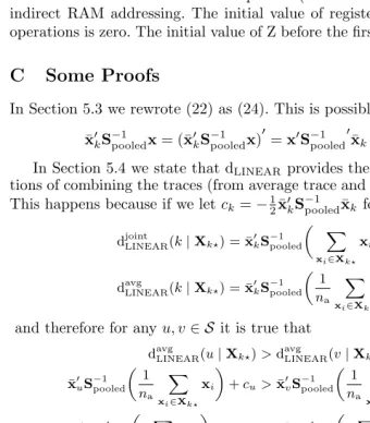
O sc il lo sc o p e 1 6 -b it d a ta MOV LDk
Fig. 4. Left: the device used during our experiments. Right: A single example trace
xr