Development and Assessment of Smoothed Particle Hydrodynamics Method for Analysis of External Hazards.

ABSTRACT

LIN, LINYU. Development and Assessment of Smoothed Particle Hydrodynamics Method for Analysis of External Hazards. (Under the direction of Dr. Nam Dinh).

improve the assessment framework by identifying and bridging the gaps of practical issues and application requirements.

Development and Assessment of Smoothed Particle Hydrodynamics Methods for Analysis of External Hazards

by Linyu Lin

A dissertation submitted to the Graduate Faculty of North Carolina State University

in partial fulfillment of the requirements for the degree of

Doctor of Philosophy

Nuclear Engineering

Raleigh, North Carolina 2019

APPROVED BY:

__________________________ _____________________________

Dr. Nam T. Dinh Dr. Igor A. Bolotnov

Committee Chair

__________________________ _____________________________

Dr. Maria N. Avramova Dr. Abhinav Gupta

ii DEDICATION

iii BIOGRAPHY

iv ACKNOWLEDGMENTS

First, I would like to appreciate Dr. Nam T. Dinh for guiding my research in the past five years. His knowledge, talent, and character have impressed me so much, and it is always my greatest honor to be one of his students. My English does not allow me to find the most accurate description for his profile in my mind, but I believe that the Chinese word “君子” and its profound meaning could be the most appropriate.

Next, I would also like to thank Dr. Igor Bolotnov, Dr. Maria Avramova, Dr. Robert Youngblood, and Dr. Abhinav Gupta for serving as my committee. Your insights and suggestions are most valuable to me. Especially, I would like to thank Dr. Robert Youngblood for opening the door to a new area.

Next, I would like to thank Dr. Curtis Smith and Steven Prescott for offering an internship opportunity to me in Idaho National Laboratory. My works there mark the start of this study. I would also like to thank Ram Sampath, Niels Montanari, Dr. Nadir Akinci, and Dr. Anh Bui for their supports and suggestions on SPH simulations. Besides, I would like to thank my friends and colleagues at North Carolina State University, Goujing Hou, Han Bao, Chih-Weih Chang, Yangmo Zhu, Yang Liu, Jun Fang, Yuwei Zhu, Hao-Ping Chang, Jinyong Feng, Botros Hanna, Paridhi Athe, Joomyung Lee, Xu Han, Alp Tezbasaran, Anil Gurgen, Nadish Saini, and many others. It has been a pleasure for me to work with you in the past five years.

Finally, I would like to give my special thanks to my parents and my beloved Mengnan for your support and accompany.

v TABLE OF CONTENTS

List of Figures ... viii

List of Tables ... xii

Nomenclature ... xiv

1. Introduction ... 1

1.1. NPPs’ Risk due to External Hazards ... 2

1.1.1. Risk of Flooding Hazards ... 2

1.1.1.1. Flooding Hazards due to Dam Failure ... 3

1.1.1.2. Flooding Hazards due to Tsunami ... 5

1.1.1.3. Flooding Hazards due to Surge ... 6

1.1.2. Risk of High Wind Hazards ... 8

1.2. Risk Analysis for External Hazards ... 9

1.2.1. Probabilistic Risk Analysis (PRA)... 10

1.2.2. Risk Informed Safety Margin Characterization (RISMC) ... 14

1.3. Model Validation and Uncertainty Quantification (VUQ) ... 17

1.3.1. Model Validation Framework ... 18

1.3.1.1. Validation of Computational Fluid Dynamics (CFD) ... 18

1.3.1.2. CSAU/EMDAP ... 20

1.3.1.3. Predictive Capability Maturity Model ... 22

1.3.2. Uncertainty Quantification... 23

1.3.3. Decision Analysis ... 25

1.3.4. Uncertainty in Decision Analysis ... 26

1.4. Summary Remarks ... 29

2. Dissertation Background ... 31

2.1. Motivation, Objective, and Technical Approach ... 31

2.2. Dissertation Conditions and Assumptions ... 32

2.3. Dissertation Overview and Outline ... 36

3. Smoothed Particle Hydrodynamics (SPH) ... 38

3.1. State of the Art ... 38

3.2. SPH in Fluid Simulations... 43

vi

3.2.2. Laminar Flow Modeling ... 44

3.2.3. Turbulent Flow Modeling ... 45

3.2.4. Fluid-Structure Interactions ... 47

3.3. Theoretical Error Analysis ... 48

3.3.1. Truncation Error Analysis... 48

3.3.2. Discretization Error Analysis ... 52

3.3.3. Simulation Error Analysis... 55

3.4. Summary Remarks ... 57

4. SPH Credibility Assessment with EMDAP framework ... 59

4.1. Establish Requirement for Evaluation Model Capability ... 60

4.1.1. Identify and Rank Key Phenomena and Processes ... 61

4.1.2. Performance Measurement Standards ... 66

4.2. Develop Assessment Base and Evaluation Model ... 69

4.3. Assess Evaluation Model Adequacy ... 73

4.3.1. External-Flooding Scenario ... 74

4.3.1.1. Dam Break ... 74

4.3.1.2. Moving Solids in Static Fluid ... 81

4.3.2. High-Wind Scenario ... 88

4.3.2.1. Flow over Obstacle ... 88

4.3.2.2. Cavity Flow ... 92

4.3.3. Summary of Assessment Results ... 97

4.4. Scaling Analysis... 97

4.5. Adequacy Decision ... 101

4.6. Issues and Challenges ... 103

4.7. Summary Remarks ... 105

5. Validation Framework for RISMC Methodology ... 107

5.1. Sufficient Accuracy ... 107

5.1.1. Technical Development ... 107

5.1.2. Case Study ... 112

5.1.2.1. Scenario Description ... 112

5.1.2.2. Vent Overflow Sufficient Accuracy ... 115

vii

5.1.3. Findings and Issues ... 125

5.2. Predictive Capability Maturity Quantification by Bayesian Network ... 126

5.2.1. Technical Development ... 127

5.2.2. Case Study ... 133

5.2.2.1. PCMQBN for Landscape Overflow Model ... 134

5.2.2.2. PCMQBN for Core Flow Pressure Loss Model ... 137

5.2.3. Findings and Issues ... 140

5.3. Local Data-Driven Uncertainty Quantification ... 142

5.3.1. Technical Development ... 142

5.3.2. Case Study ... 147

5.3.3. Findings and Issues ... 153

5.4. RISMC Model Validation Framework ... 154

5.4.1. Blocks Improved by Formalized Methodologies ... 155

5.4.2. Scoping Developments for Validation Data Plan and Uncertainty Scaling ... 156

5.4.3. Extended Framework Development ... 161

5.5. Issues and Challenges ... 163

5.6. Summary Remarks ... 164

6. Conclusion: Summary of Findings and Future Work ... 166

6.1. Summary ... 166

6.2. Contributions... 171

6.3. Recommendations for Future Work... 174

7. References ... 176

viii LIST OF FIGURES

Figure 1-1: Picture of Fukushima accident from BNN [1]. ... 1

Figure 1-2: NRC post-Fukushima safety enhancements [12]. ... 3

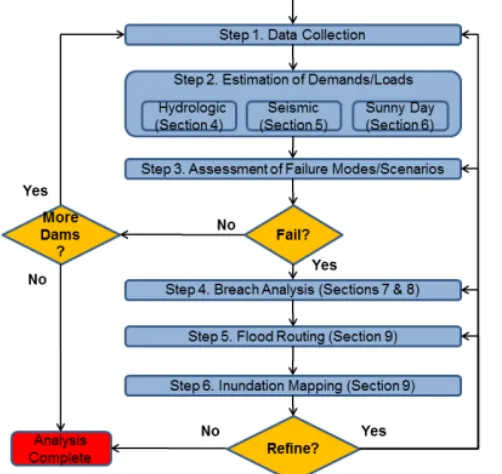
Figure 1-3: Overview of detailed dam failure flood hazard analysis from figure 2 of JLD-ISG-2013-01 [10]. ... 4

Figure 1-4: An illustration of the dam breaching process by overtopping: (a) rills and cascade of small overfalls at t 1⁄4 7 min; (b) consolidation of small overfalls at t 1⁄4 13 min; (c) headcut at downstream crest at t 1⁄4 16 min; (d) headcut at upstream crest at t 1⁄4 31 min; (e) flow through breach at t 1⁄4 40 min; (f) transition to final breach stage at t 1⁄4 51 min [14]. ... 5

Figure 1-5: Picture of 2004 Indian ocean tsunami [15]. ... 6

Figure 1-6: Illustration of 200 synthetic storm tracks [17]. ... 7

Figure 1-7: Structural damage to Turkey Point unit 1 exhaust stack [24]. ... 9

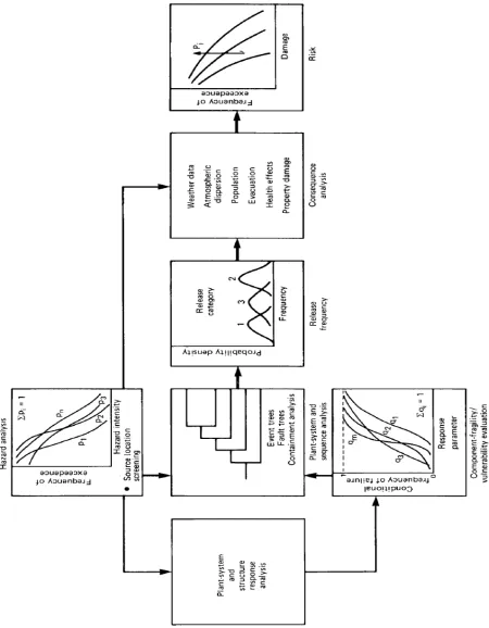
Figure 1-8: Risk-assessment procedure for external events from figure 10-1 of NUREG/CR-2300 [27]. ... 11

Figure 1-9: Simple representation of load and capability in regular PRA (left) and RISMC (right) analysis. The shaded region in right plot is where the load exceeds capacity and risk could possibly happens. ... 15

Figure 1-10: Flowchart of applying RISMC in external flooding analysis by C. Smith, et al. [26]. ... 16

Figure 1-11: NEUTRINO simulation for the Fukushima tsunami event [39]. ... 16

Figure 1-12: Flowchart of CFD V&V and Uncertainty Quantification (UQ) Process. ... 19

Figure 1-13: Demonstration of validation tiers... 20

Figure 1-14: EMDAP validation framework. ... 22

Figure 1-15: Schematic flowchart of uncertainty analysis, including examples of inputs and outputs for each component. ... 25

Figure 1-16: Illustration of pyramid-type validation framework, and its connection to adequacy decision, model credibility, and the safety decision. Letter “E” stands for Evidence, while letter “A” stands for Argument. Both evidence and argument are for model credibility/uncertainty. After the integration by validation framework, an adequacy decision will be made with respect to the selected model and application. If the model turns to be adequate, the credibility/uncertainty information will be fed into the safety analysis framework any safety-related decision. ... 30

Figure 2-1: An illustration of dissertation structures and flowcharts. ... 37

Figure 3-1: Demonstration of particles inside one support region with radius ht. ... 53

Figure 3-2: Comparison of SPH simulation and analytical solution of Poiseuille flow. ... 56

Figure 3-3: Plot of convergent rate against particle size in SPH simulation. ... 57

Figure 4-1: Demonstration of adequacy decision process. ... 60

Figure 4-2: Demonstration for a postulated external flooding scenario induced by dam failures. A full-scale simulation is prepared with NEUTRINO software package [78]. ... 71

ix Figure 4-4: Evolution of the water collapse and interaction with the column simulated by

NEUTRINO. (a) start of simulation; (b) primary wave hitting dam structure; (c) wave reflected; (d) Reflected wave hitting dam structure. ... 76 Figure 4-5: Particle size convergence plot for force magnitude and contacting time of

primary and reflected wave. ... 77 Figure 4-6: Plot of relative error against computing time for force magnitude and

contacting time of primary and reflective wave. ... 78 Figure 4-7: Evolution of the water collapse and interaction with the column based on

Aureli’s setups. (a) start of simulation; (b) primary wave hitting dam structure. ... 79 Figure 4-8: Comparison of the measured against SPH predicted peak force with different

dimensionless ratio 𝑥𝑥 ∗. ... 80 Figure 4-9: Plot of 𝐿𝐿1 relative error norm for predicting the peak force versus the

dimensionless ratio 𝑥𝑥 ∗ with particle size as 0.02m. ... 80 Figure 4-10: Dimensions of the water tank and cube in the falling experiment (left) and the

floating experiment (right). The density of water is 1000 𝑘𝑘𝑘𝑘/𝑚𝑚3. ... 82 Figure 4-11: Transient plots of falling solids in fluid from NEUTRINO. ... 82 Figure 4-12: Comparison of vertical displacement of falling block simulated NEUTRINO

with three particle sizes. ... 83 Figure 4-13: Transient plots of floating solids in fluid from NEUTRINO. ... 84 Figure 4-14: Comparison of vertical displacement of floating block simulated by

NEUTRINO. ... 85 Figure 4-15: Setup and dimensions of channel flow with block. ... 88 Figure 4-16: Comparison of velocity profile with and without particle shifting algorithm

along vertical probe behind the block at x=0.38m. ... 89 Figure 4-17: Velocity profile along vertical probe behind the block at x=0.38m. ... 89 Figure 4-18: Plot of relative error for the minimum velocity for SPH with and without the

particle shifting algorithm at x = 0.38m... 90 Figure 4-19: The particle distribution of SPH simulation for the lid-driven cavity flow. The

red particles represent lid that is driven by a constant speed, black particles represent the stationary boundaries, while the blue particle represent the fluid. .. 93 Figure 4-20: Comparison of velocity profiles from OpenFOAM and experimental

measurements along the vertical centerline (left) and horizontal centerline (right) when 𝑅𝑅𝑅𝑅𝑅𝑅= 10000. ... 94 Figure 4-21: Velocity profile of different particle size on the vertical centerline with

𝑅𝑅𝑅𝑅𝑅𝑅=100 (left) and 𝑅𝑅𝑅𝑅𝑅𝑅 =1000 (right). ... 95 Figure 4-22: Plot of 𝐿𝐿1 relative error norm for x-direction velocity field versus the Reynolds

number. ... 95 Figure 4-23: Particle distribution of SPH simulation with Re=10000. ... 96 Figure 5-1: Demonstration of landscape (left) and vent (right) overflow scenario. ... 113 Figure 5-2: Transient plot of water depth for the synthetic overflow scenario with the

maximum depth 𝐻𝐻0 = 2𝑚𝑚. ... 114 Figure 5-3: Demonstration of error distribution for high maturity, low maturity, and 50%

belief on high maturity. ... 116 Figure 5-4: Plot of predicted response time against the belief on the model’s high maturity

x where the response time should be higher than 30min. The point that two lines intercept is defined as critical belief, where the safety goal can always be

satisfied given the belief is higher than the critical value. ... 117

Figure 5-5: Estimated critical belief on high-maturity model versus the initial flood depth, the region on the left of function line is the acceptance domain. The regions in red boxes suggest the situations where subjective beliefs on model maturity levels do not affect the satisfaction of safety goal. The bottom box indicates the situations where safety margins of facilities or components are much more than the model uncertainties, while the upper box indicates that the margins are less than the model uncertainty. ... 118

Figure 5-6: Demonstration of risk-informed load and capability distributions for (a) scenarios with no overlap between load and capacity distribution (b) scenarios where load distribution is so wide that it fully covers the capacity distribution. Scenario (a) corresponds to the region ①, and the safety goal is always satisfied given all ranges of subjective beliefs on the model’s maturity. Scenario (b) corresponds to the region ②, and the safety goal can never be satisfied by whatever subjective beliefs. ... 119

Figure 5-7: Demonstration of error distribution for high maturity, low maturity, and 50% belief on high maturity. ... 120

Figure 5-8: Plot of predicted response time against the belief on the model’s high maturity level when 𝑄𝑄 = 0.5𝑚𝑚3/𝑠𝑠. The dashed line represents the safety requirement where the response time should be higher than 30min. The point that two lines intercept is defined as critical belief, where the safety goal can always be satisfied given the belief is higher than the critical value ... 121

Figure 5-9: Estimated critical belief on high-maturity model versus the flow rate, the region on the left of function line is the acceptance domain. ... 122

Figure 5-10: Demonstration of error bounds for parameter 𝛼𝛼 and 𝛽𝛽. ... 123

Figure 5-11: Comparison of errors bounds for predicting the flow rate 𝑄𝑄 with inferred parameters against the error bounds with direct sampling. ... 124

Figure 5-12: Relationship of subjective belief and response time with respect to three uncertain scenarios. Comparisons are also made for each scenario by using the inferred parameters and the direct sampled prediction error. ... 125

Figure 5-13: Example of Bayesian network for a “separate” code adequacy assessment with equal and unequal weights. The plot is prepared with AgenaRisk [164] ... 132

Figure 5-14: Demonstration of phenomenon decomposition for flow over the broad-crested weir. The IET measures the flow directly with respect to upstream water depth, while two SETs measure the discharge coefficient and the approach velocity coefficient respectively. ... 135

Figure 5-15: Plot of model predictions for SET and IET calibrated parameters versus experimental data. (a) discharge coefficient; (b) approach velocity coefficient; (c) flow rate. ... 136

Figure 5-16: Scheme of validation decision and the performance of Bayesian Sensitivity Study. ... 141

Figure 5-17: Illustration of forward and inverse uncertainty quantification. ... 144

Figure 5-18: Illustration of workflow for global and local data-driven UQ approach. ... 145

xi Figure 5-20: Time averaged L2 relative error norm by four time-windows versus physical

time for at fully developed state with 𝑅𝑅𝑅𝑅𝑅𝑅= 10000. ... 149 Figure 5-21: Comparison of 𝑉𝑉𝑥𝑥 at the vertical centerline. ... 149 Figure 5-22: Histogram of PEML predicted uncertainty when the training group contains a

single simulation and the target group has 𝑅𝑅𝑅𝑅𝑅𝑅 − 𝑡𝑡𝑡𝑡𝑡𝑡𝑘𝑘𝑅𝑅𝑡𝑡 = 10000. ... 152 Figure 5-23: Histogram of PEML predicted uncertainty when the target group has 𝑅𝑅𝑅𝑅𝑅𝑅 −

𝑡𝑡𝑡𝑡𝑡𝑡𝑘𝑘𝑅𝑅𝑡𝑡= 5000. ... 152 Figure 5-24: A schematic flowchart of the improved EMDAP framework. The solid blocks

are mainly inherited from the well-established EMDAP framework, and three of them have been improved with new methodologies (in bold font). The definitions and case studies of bold methodologies have been demonstrated in this study. The scopes and requirements of dash blocks have been defined for the dashed blocks. ... 155 Figure 5-25: Demonstration of maturity and code adequacy improvement by a “postulated”

model... 157 Figure 5-26: Decision tree for calculating the expected increase in the monetary values by

having a postulated new model rather than having the IET-calibrated model. .. 158 Figure 5-27: Plot of NMSE for the corrected low-fidelity simulation against the Reynolds

ratio 𝑡𝑡 ∗ and K-L Divergence when the target scenario has 𝑅𝑅𝑅𝑅𝑡𝑡𝑡𝑡𝑡𝑡𝑘𝑘𝑅𝑅𝑡𝑡= 10000. ... 161 Figure 5-28: Risk-informed Evaluation Model Development and Assessment Process.

Orange boxes denote developments in the project and indicate EMDAP elements where the advances are expected to impact [182]. “Reqs” is the abbreviation for “Requirements”; VDMS refers to Validation Data Management System; SBS refers to Simulation-Based Scaling; DDM refers to Data-Driven Modeling; ROM refers to Reduced Order Modeling. ... 162 Figure 5-29: Schematic illustration of validation pyramid guided by the concept of sufficient

xii LIST OF TABLES

Table 1-1: Tornado strike frequencies for ESBWR in high-wind events [25]. ... 13 Table 1-2: Definition of uncertainty levels with respect to the knowledge assumed about

the various aspects of a decision-making problem [68]... 28 Table 2-1: Important conditions and assumptions with respect to aspects of investigation.

... 33 Table 3-1: Summary of some popular SPH treatments in Computational Fluid Dynamics

(CFD). ... 42 Table 3-2: Review and comparison of LES and RANS k- ε model applied in SPH. ... 47 Table 4-1: PIRT and lists of numerical benchmarks designed for each phenomenon in

external flooding scenario. ... 64 Table 4-2: IRT and lists of numerical benchmarks designed for each phenomenon in high

wind scenario. ... 65 Table 4-3: Simulation code accuracy standards measured by error in predicting selected

QoIs. ... 67 Table 4-4: Attributes and criteria of systematic scaling analysis. ... 68 Table 4-5: Scenario configurations, NEUTRINO setups, and predicted FoMs. ... 71 Table 4-6: Numerical benchmarks for all high-rank phenomena. Benchmarks in blue and

italic fonts are investigated but not discussed in this study. ... 73 Table 4-7: Simulation parameters with 20% bounded absolute relative error for the case

of dam break. ... 79 Table 4-8: Simulation parameters that are scaled from numerical benchmarks to a

postulated scenario with the same dimensionless group. ... 81 Table 4-9: Particle sizes in NEUTRINO simulations for falling cube, and the absolute

relative error of each simulation in predicting the cube falling time. ... 84 Table 4-10: Particle sizes in NEUTRINO simulations for floating cube, and the 𝐿𝐿1 relative

error norm of each simulation in predicting the cube floating time and oscillation period. ... 85 Table 4-11: Simulation parameters that are scaled from numerical benchmarks to a

postulated scenario with the same dimensionless group. ... 87 Table 4-12: Simulation parameters with 30% bounded 𝐿𝐿1 relative norm for the case of

wind over block. Yellow shaded column represents the combination of parameters and models with the lowest computational cost. ... 91 Table 4-13: Simulation parameters that are scaled from numerical benchmarks to a

postulated scenario with the same dimensionless group. ... 92 Table 4-14: OpenFOAM solver information. ... 93 Table 4-15: Simulation parameters that are scaled from numerical benchmarks to a

postulated scenario with the same dimensionless group. ... 96 Table 4-16: Comparison of measured and SPH predicted QoIs for high-rank phenomena of

external-flooding and high-wind scenarios. ... 97 Table 4-17: Summary of numerical benchmarks designed for each phenomenon in

xiii phenomena “hydrodynamic force on moving structures”, the dimensionless number in application is assumed to be the same as that in validation database. For phenomena “turbulence” and “vortex shedding”, the validation database

does not cover the characteristics of application. ... 100

Table 4-18: Validation result for SPH methods in simulating the external-flooding and high-wind scenario. For each phenomenon, the particle sizes are sample, and the one with acceptable accuracy and least computational expenses are suggested. ... 102

Table 5-1: Example of maturity level and their descriptions for situations with large uncertainties due to a lack of prototypic data. The attribute is designated according to the scaling analysis... 110

Table 5-2: Comparison of Sufficient Accuracy concept against Risk-Informed/Risk-Oriented concept. ... 112

Table 5-3: Definition of sufficient accuracy and their probability density distribution for model prediction error... 115

Table 5-4: Definition of maturity level and their probability density distribution for model prediction error... 120

Table 5-5: Grade table for validation experiment. ... 129

Table 5-6: An example of monetary rewards assigned to each maturity level ... 133

Table 5-7: Value of model parameters calibrated based on SET and IET. ... 136

Table 5-8: EMVs of the model adequacy for different combinations of model and weight factor. ... 137

Table 5-9: R/S/U grades and weight factors for data from PISA and KALLA facility. ... 138

Table 5-10: EMVs of the code adequacy for six combinations of wall friction and form loss coefficient model. ... 139

Table 5-11: Summary of simulation ID and configurations. Dynamic viscosity is currently the only variables being changed. ... 147

Table 5-12: Summary of PEML results with Random Forest as the machine-learning engine. ... 151

xiv NOMENCLATURE

CDF Core Damage Frequency

CFL Courant-Friedrichs-Lewy

CFD Computational Fluid Dynamics

CSAU Code Scaling, Applicability, and Uncertainty

DoE Department of Energy

DNS Direct Numerical Simulation DPD Dissipative Particle Dynamics

EF Enhanced Fujita

EMDAP Evaluation Model Development and Assessment Process

EMV Expected Monetary Value

EOS Equation of State

ESBWR Economic Simplified Boiling Water Reactor EVSI Expected Value of Sample Information

FoM Figure of Merit

FV Finite Volume

GLM Generalized Langevin Model

HHA Hierarchical Hazard Assessment IET Integrated Effect Test

ISPH Incompressible SPH

IISPH Implicit Incompressible SPH IRP Integrated Research Project

LES Large Eddy Simulation

LOOP Loss of Offsite Power

LWRS Light Water Reactor Sustainability

MD Molecular Dynamics

NOAA National Oceanic and Atmospheric Administration

NPP Nuclear Power Plant

NRC Nuclear Regulatory Commission PCMM Predictive Capability Maturity Model

PCMQ Predictive Capability Maturity Quantification

PCMQBN PCMQ by Bayesian Network

PDE Partial Differential Equation PDF Probability Density Function

PEML Physics-Evaluated Machine Learning PTHA Probabilistic Tsunami Hazard Assessment PIRT Phenomenon Identification and Ranking Table PRA Probability Risk Analysis

QoI Quantity of Interest

RANS Reynold Averaged Navier Stoke

REMDAP Risk-informed EMDAP

RISMC Risk Informed Safety Margin Characterization R/S/U Relevance/Scaling/Uncertainty

xv

SET Separate Effect Test

SPH Smoothed Particle Hydrodynamics

SPS Sub-Particle Scale

SSC System, Structure and Component

TW Time Window

UQ Uncertainty Quantification

V&V Verification and Validation

VDP Validation Data Plan

1

1. INTRODUCTION

On March 11, 2011, Tōhoku earthquake occurred near Japan and triggered a 13-15m high tsunami. In Ōkuma, the wave overtopped the seawall of the Fukushima Daiichi Nuclear Power Plant, flooded and disabled the plant’s electrical system. From March 12 to March 15, the insufficient cooling leads to core meltdowns, explosions and release of radioactive material in Unit 1, 2 and 3 (Figure 1-1). Since this accident, increased attentions are paid on to the risk assessment of Nuclear Power Plant due to external hazards. In this chapter, external hazards, including flooding and high wind, are introduced. The well-established Probabilistic Risk Analysis (PRA) method and a novel Risk-Informed Safety Margin Characterization (RISMC) methodology are introduced as the tools of risk analysis and safety management. Since physical models and computational software are applied in risk analysis to capture transient phenomena during accident scenarios, validation framework designed to assess the accuracy of model and software, has been constructed and described in this chapter.

2 1.1. NPPs’ Risk due to External Hazards

In this study, two major external hazards are considered: flooding and high wind. Scenarios of high wind have been analyzed for two decades. Required by U.S. Nuclear Regulatory Commission (NRC), the risk of high wind, including the direct impact and wind-generated missiles, are investigated with PRA and presented in the design control document for the licensing of newly designed NPP [2] [3]. Besides, extensive preparations for the hurricane are required to make for both Nuclear Power Plant (NPP) owner and operator before the hurricane’s landfall. While for flooding scenarios, the safety analysis relies on external-hazard PRA with designated event progressions [4].

1.1.1. Risk of Flooding Hazards

3 plant response to the flood hazard, considering multiple and diverse capabilities such as physical barriers, temporary protective measures, and operational procedures [9].” Besides, two specific guidance is made for the assessment of flooding hazards due to dam failure [10] and for performing a tsunami, surge, or seismic hazard assessment [11]. Detailed descriptions and proposed safety strategies are further introduced in the following sections.

Figure 1-2: NRC post-Fukushima safety enhancements [12].

1.1.1.1. Flooding Hazards due to Dam Failure

4 Figure 1-3: Overview of detailed dam failure flood hazard analysis from figure 2 of

JLD-ISG-2013-01 [10].

5 Figure 1-4: An illustration of the dam breaching process by overtopping: (a) rills and cascade of small overfalls at t 1⁄4 7 min; (b) consolidation of small overfalls at t 1⁄4 13 min; (c) headcut at

downstream crest at t 1⁄4 16 min; (d) headcut at upstream crest at t 1⁄4 31 min; (e) flow through breach at t 1⁄4 40 min; (f) transition to final breach stage at t 1⁄4 51 min [14].

1.1.1.2. Flooding Hazards due to Tsunami

6 required as one part of tsunami hazard reevaluations. In some well-established frameworks, the tsunami is generated according to historical data, and it is obtained from the regional or site-specific survey. Next, the computational model is applied to simulate the tsunami propagation. U.S. NRC has suggested several packages based on the shallow-water equation, including MOST, COMCOT and TSUNAMI2. Finally, wave and inundation effects, including the hydrostatic/hydrodynamic forces, debris projectiles, and sediment erosion, are required to be analyzed. However, most of them are analyzed independently by statistical tools, and there is no systematic analysis for capturing flooding progressions and flood-structure interactions.

Figure 1-5: Picture of 2004 Indian ocean tsunami [15].

1.1.1.3. Flooding Hazards due to Surge

7 Probable Maximum Hurricane (PMH) and Joint Probability Method (JPM) are used for generating synthetic hurricanes (Figure 1-6). Meanwhile, ANSI/ANS-2.8-21992 and Empirical Simulation Technique (EST) are used to generate synthetic extra-tropical storms and squall lines. As for the surge propagation, Advance CIRCulation Surge Model (ADCIRC) model, by USACE Dredging Research Program, is used to simulate tidal circulation and storm-surge propagation over very large computational domains with complex costal configurations [16].

Figure 1-6: Illustration of 200 synthetic storm tracks [17].

8 1.1.2. Risk of High Wind Hazards

9 Figure 1-7: Structural damage to Turkey Point unit 1 exhaust stack[24].

For identifying and managing safety margins of NPP during external hazards, risk analysis is required for measuring the probabilities and consequences of designated scenarios. The following section reviews the existing risk analysis methodologies in the nuclear discipline.

1.2. Risk Analysis for External Hazards

10 comprehensive descriptions of accident initiating, progression, and consequence. And the results are expected to be more informative and effective for risk management and mitigation purposes.

1.2.1. Probabilistic Risk Analysis (PRA)

11 Figure 1-8: Risk-assessment procedure for external events from figure 10-1 of

12 Five major steps are included in the PRA analysis for external hazards, detailed descriptions can be found as follows:

• Hazard analysis – to determine the frequency of occurrence for different intensities of high wind. The result is to generate one or more high wind hazard curves that are applicable to the NPP;

• Plant-system and structure response analysis – to translate the hazard input into the responses acting on a component. The result is frequency distribution of the responses (e.g. force acting on SSCs by winds) for each high wind intensity,

• Evaluation of the fragility and vulnerability of components – to determine the conditional frequency of components’ failure given a value of the response parameter. The result is to generate a fragility curves for the various SSCs that are susceptible to the effects of the winds or wind generated missiles;

• Plant system and sequence analysis – to evaluate the risk initiated by high wind or LOCA initiating event induced or caused by high wind. The result is to develop hazard specific fault tree/event tree model,

• Consequence analysis.

Of the five steps of high wind-PRA, the most challenging part is assessing the possibility and impact of the hazard, including the direct impacts of the wind and the impacts of wind-generated missiles. For the PRA study for ESBWR, a tornado strike initiating event frequency is calculated with the methodology in NUREG/CR-4461 [28] and the model for U.S. Central region (Eq. 1).

𝑃𝑃(𝑢𝑢 ≥ 𝑢𝑢0) =𝑃𝑃𝑝𝑝exp�− �𝑢𝑢0_𝑡𝑡−65 𝑝𝑝 �

𝑏𝑏𝑝𝑝

�+𝑃𝑃𝑙𝑙exp�− �𝑢𝑢0−_𝑡𝑡 65 𝑙𝑙 �

𝑏𝑏𝑙𝑙

� Eq. 1

13 1-1) and substitute into the event tree for Loss of Preferred Power Event Tree. The Enhanced Fujita (EF) represents the tornado category classified by the NOAA’s National Weather Service [29].

Table 1-1: Tornado strike frequencies for ESBWR in high-wind events [25]. Tornado Event Tornado Strike Frequency (events/yrs)

EF2/ EF3 9.68E-05

EF4 4.42E-05

EF5 5.02E-07

It turns out that the total Core Damage Frequency (CDF) for both at-power and shutdown conditions induced by high wind is 4.80 × 10−8_{/𝑦𝑦𝑡𝑡 with a CDF of 8.51 × 10}−9_{/𝑦𝑦𝑡𝑡 for at-power} operations and a CDF of 3.95 × 10−8_{/𝑦𝑦𝑡𝑡 for shutdown operations. These results are acceptably} low and meet the NRC goals.

The missile strike problem is described in NUREG-0800, in which spectrums of missiles are provided [30]. Recently, some initial work has been done by EPRI and computer codes like TORMIS [31] and TORRISK [32] are developed based on the Monte Carlo Method. However, U.S. NRC has described some issues that have occurred in the use of these codes and the interpretation of results, TORMIS/TORRISK still needs detailed analysis to obtain regulatory approval [33]. Another development is made by Westinghouse Electric Corporation for a tool named “Tornado Missile Strike Calculator (TMSC)”. It is an application based on Microsoft Excel, and it uses statistical correlations to estimate the missile strike probability [34]. However, it does not explicitly model the physics of high wind, and it might only be applicable for addressing issues within its documented validation basis.

14 field, an F5 tornado will only experience F5 force winds over roughly 15% of its track. Furthermore, the direct effects of the wind are combined with other correlated hazards such as locally intense precipitation and wind generated missiles. However, it turns out that such resolution and complexity are hard to be achieved with the existing methods and tools in the regular high-wind PRAs. New approaches that are capable of accurately capturing multi-physics interactions and dynamically tracking the failure probability are needed.

1.2.2. Risk Informed Safety Margin Characterization (RISMC)

15 Figure 1-9: Simple representation of load and capability in regular PRA (left) and RISMC (right) analysis. The shaded region in right plot is where the load exceeds capacity and risk could

possibly happens.

Note that for the RISMC analysis in practical situations, the simple load-capacity approach turns to be oversimplified since load and capability can be correlated in some scenarios. It has been argued that though the risk-informed concept that margin needs to be quantified with probability remains valid, it is not applicable to compute load and capacity curve separately as if they are independent [36]. As a result, it is suggested that limiting surface should be employed to determine the failure probability [37].

16 Figure 1-10: Flowchart of applying RISMC in external flooding analysis by C. Smith, et al.

[26].

Figure 1-11: NEUTRINO simulation for the Fukushima tsunami event [39].

17 assessments have been performed for SPH and NEUTRINO [26], however, due to the complexity of physics and phenomenon, a comprehensive validation is still needed to accurately characterize the uncertainty and credibility of simulations. At the same time, the factor of computational efficiency also needs to be considered. Although SPH is comparable to DNS with sufficiently refined particles, it is not practical to perform RISMC analysis with DNS configurations. Besides, as a simulation tool for engineering and industrial applications, the validation goal should be adapted to the contextual requirements, including safety margins, probability of occurrence, consequence, and so on. Therefore, the validation frameworks and standards that guide SPH assessments should be application-oriented and error-tolerant. Meanwhile, the validation results from the framework should be directly used by the applications, like engineering design, safety analysis, etc.

In conclusion, comparing to the statistical analysis by the well-established PRA, RISMC relies on advanced three-dimension and multi-physics simulation tools. In return, RISMC is expected to provide comprehensive and detailed descriptions for the accident initiation and progression. The product of RISMC is also expected to be more effective and informative for the purposes of risk management and mitigation. However, the simulation tools need to be systematically validated such that the predicted System Quantity of Responses (SQR) from simulations are convincing and reliable. Besides, considering the purposes of safety analysis and management, the validation process needs to investigate how model uncertainties affect the safety decisions or facility designs such that the validation goal can be properly designated.

1.3. Model Validation and Uncertainty Quantification (VUQ)

18 mechanical engineering, and nuclear engineering. Moreover, since validation is essentially a decision-making process that aims to determine the credibility of simulation models, this chapter briefly discusses the concept of decision analysis and uncertainties in decision-making. The goal of these reviews is to gain insights from various disciplines and identify potential resolutions that could help the achievement of objectives for this study.

1.3.1. Model Validation Framework

In addition to the AIAA Guidance for CFD code validation [41], U.S. NRC suggests a validation framework called Evaluation Model Development and Assessment Process (EMDAP), which is mainly designed for the system code for transient and accident analysis of NPP [42]. Besides, to support the decision-making that relies on the model credibility, a framework of Predictive Capability Maturity Model (PCMM) is developed to assess the quality of M&S activities with maturity levels.

1.3.1.1. Validation of Computational Fluid Dynamics (CFD)

19 hardware is fabricated and inspected. The purpose is to isolate each element of a complex system so that “critical evaluations of mathematical models or sub-models can be evaluated [43]”. Besides, it is also suggested that repeated experiments on different facilities are needed to ensure the identification of systematic errors. However, some parameters that are needed for the CFD simulation of benchmark cases and unit problems are not measured. Then the analyst should assume these quantities. As for the large-scale testing of the complete system and subsystem cases, also known as Integral Effect Tests (IETs), only the Quantity of Interests (QoIs) for engineering purposes are measured. Because the large-scale tests are usually expensive and complex, complete measurements of all physical parameters are hard to achieve. In addition, for the risk analysis related to NPP and the external hazards, validation experiments of the complete system are impossible to achieve.

20 Figure 1-13: Demonstration of validation tiers.

In general, a “divide-and-conquer” strategy is used in the CFD validation with simplistic treatment for multi-physics problems. Note that the concept of scale separation is applied for the hierarchy structures. Due to the simplistic treatment of the multi-scale phenomena, such framework is suitable for the weakly non-linear system. For the application of nuclear engineering, where the scale could range from kilometer (flooding) to micrometer (boiling), the technique of divide-and-conquer may not very applicable. Besides, the CFD validation framework proposed by AIAA is mainly designed for aerospace engineering, where the accuracy requirements are very high. While for the risk analysis in nuclear engineering, the acceptance range for the accuracy of nuclear reactor system code is not as high as the aerospace. As a result, a validation framework designed for nuclear risk analysis is developed by U.S. NRC.

1.3.1.2. CSAU/EMDAP

21 Criteria”. The objective is to demonstrate a method that “can be used to quantify uncertainties as required by the best-estimate option described in the NRC’s 1988 revision to the ECCS Rule (10 CFR 50.46) [42]”. CSAU methodology is mainly composed by three elements [45]: (1) requirements and code capability; (2) assessment and ranging of parameters; (3) sensitivity and uncertainty analysis; The first element aims to identify the code applicability and potential code limitations for the particular scenarios. This is usually achieved with a phenomenon identification and ranking process, (e.g., Phenomenon Identification and Ranking Table (PIRT) [46]), such that the assessment process can be sufficient and efficient. The product of the first element is a hierarchy of relevant tests for the code validation, including the SETs, mixing effect tests (METs), and IET. The second element aims to assess the capability of the code by comparing simulation results against experimental data. The scaling methodology is needed in this element to guide the development of simulation codes and assess the code scale-up capability. The third element aims to assess the uncertainty due to the code limitations, scaling distortions, data quality, and so on. Usually, the second and third element are performed at the same time and the ultimate product is a simple and direct statement of the code uncertainty or credibility in the primary safety criterion (e.g. the Peak Cladding Temperature (PCT)). For obvious and inevitable limitations in knowledge, a conservative margin is added to compensate for the effect of epistemic uncertainty.

22 of VUQ, they have a vague classification between the verification and validation. CSAU has been successfully applied to the RELAP-5 simulation code for the Small Break Loss-of-Coolant Accidents of AP600 [47], while EMDAP has not been widely applied. Figure 1-14 shows the overall diagram of the EMDAP process and the relationships among its elements [42]:

Figure 1-14: EMDAP validation framework.

1.3.1.3. Predictive Capability Maturity Model

23 the corresponding model is selected. Also, based on the nature and consequence of the application, requirements and targets can be designated. Next, for the chosen scenario, six attributes are designed and assessed separately: representation and geometric fidelity; physics and material model fidelity, code variation, solution verification, model validation, and uncertainty quantification and sensitivity analysis. At the same time, a qualitative assessment for each attribute is performed based on a PCMM matrix, and it characterizes each attribute with maturity levels. Finally, the model’s achieved level is compared against the target level and the decision of validation adequacy can be made. Since the final decision can either be made based on a stringent requirement or a trade-off between the fulfillment and limitation, PCMM can effectively guide the development and validation of M&S tools. In addition, PCMM presents a formal definition for credibility assessment using the maturity level and it also explicitly distinguishes the difference between verification and validation. Though the maturity descriptor of PCMM includes statements of IETs and SETs, the scaling analysis and the hierarchical structure are not explicitly discussed. As a result, the capability of PCMM is limited in validating complex systems with multiple phenomena. In 2013, PCMM has been specifically discussed in the report by U.S. NRC [49], which emphasizes the use of maturity for the model credibility assessment. CASL also adopts PCMM for assessing Multiphysics computational tools [50].

1.3.2. Uncertainty Quantification

24 limited to the treatment for epistemic uncertainty, and there are two approaches for representing an epistemic uncertainty: interval with no associated Probability Distribution Function (PDF); or degree of belief by a PDF. The latter approach is usually known as the Bayesian approach to UQ, while the former one is usually based on the interval arithmetic, where no value is truer than any other value. Detailed discussion is beyond the scope, and this study mainly investigates the Bayesian approach.

25 Figure 1-15: Schematic flowchart of uncertainty analysis, including examples of inputs and

outputs for each component.

1.3.3. Decision Analysis

26 Also, by formally representing the decision problems, decision analysis can produce alternatives that are logically consistent and therefore persuasive [62]. In this study, for model validation purposes, decision analysis aims to improve the assessment for model credibility and identification for validation criteria such that their processes are transparent, consistent, and robust. Various techniques have been developed to represent the validation decision with formal and mathematical languages, including risk-based method [63] and hypothesis testing [63] [64] [65].

1.3.4. Uncertainty in Decision Analysis

The notion of uncertainty has been discussed and emphasized in various fields, including engineering, statistics, psychology, and economics, etc. In each discipline, a specific context and scope can be provided in terms of problem, theory, methods, and tools, etc. In this chapter, uncertainty will be discussed from a broader point of view, where uncertainty can be much larger. Generally, uncertainty can be defined as limited knowledge. At the same time, in decision-making process, the extent of uncertainty involves levels of subjective confidence since it is related to the satisfaction with existing knowledge. In addition, the uncertainty is colored by the underlying values and perspectives of the decision maker involved in the decision-making process, and the decision options available to them.

27 sensitivity analysis for all model parameters. Level 2 uncertainty is the situation that decision-makers are not certain about the future state. And such uncertainties are usually captured in the form of multiple forecasts (scenarios) with associated probabilities. Level 2 uncertainty can be adequately described in statistical terms. In risk analysis, event/fault tree is usually used for determining the possible outcomes and the corresponding likelihoods. Level 3 uncertainty represents the situation where decision-makers can create multiple alternatives and rank the alternatives in terms of perceived likelihood rather than probabilities [70]. The alternatives represent some different parametrizations of the system model, alternative sets of outcomes, and/or different conceivable sets of weights. At the same time, the likelihood is usually created based on available knowledge and information for these alternatives. For Level 3 uncertainty, the future states can usually be represented by more than one alternative, which is often developed based on various assumptions. Furthermore, at least one or the range of model predictions can cover the real future states. In scientific computing, the alternatives are characterized with mathematical models. Level 4 and Level 5 uncertainty is usually defined as “deep uncertainty” under which conditions that “analysts do not know or the parties to a decision cannot agree upon (1) the appropriate models to describe interactions among a system’s variables, (2) the probability distributions to represent uncertainty about key parameters in the models, and/or (3) how to value the desirability of alternative outcomes” [71]. To be specific, the phrase of “do not know” refers to level 5 uncertainty, while “cannot agree upon” refers to Level 4 uncertainty. In this study, focuses have been put onto Level 2 and 3 uncertainties.

28 assumptions consistent with known facts” [73]. Before making decision, the static robust approach will explore how different assumptions about future values of uncertain assumptions that affect the decisions. Scenario planning [74] is an example of such approach. It assumes that there are a range of plausible futures that can be specified well enough to identify a static decision, and it will produce acceptable outcomes in most of them. The fourth approach aims to generate decisions that can adapt to changing conditions over time. Since this approach is proposed mainly for Level 5 uncertainty, which is beyond the scope of this study, no detailed discussion will be further made.

Table 1-2: Definition of uncertainty levels with respect to the knowledge assumed about the various aspects of a decision-making problem [68].

Co mp le te C er ta in ty

Level 1 Level 2 Level 3 Level 4 Level 5

Tot al ignor anc e Future State A clear future with sensitivity Alternate future with probabilities Alternate futures with ranking A multiplicity of plausible futures no ranking Unknown future System Model A single system model

A single system model with a probabilistic parameterization Several system models, one of which is most likely Several system models, with different structures Unknown system model; know we do not know System Outcomes Point estimates with sensitivity

Several sets of point estimates with confidence intervals, with a probability attached to each set Several sets of point estimates, ranked according to their perceived likelihood A known range of outcomes Unknown outcomes; know we do not know Weights on the outcomes A single estimate of the weights

29 In conclusion, this chapter discusses and reviews state of the art for model validations. It is found that well-established validation frameworks have a pyramid structure for integrating evidence and argument related to model credibility/uncertainty. After the integration, an adequacy decision is needed to judge if the simulation tool is adequate for performing confirmatory analysis for a given application and recommended guidance. Depending on the inherent methodologies, different frameworks have their integration schemes and performance standards. In this study, two established frameworks in nuclear discipline have been reviewed. The CSAU/EMDAP framework emphasizes the scaling methodology for bridging the gaps between the validation database and application scenarios. The PCMM formalizes the model validation as a decision-making process and assesses the model adequacy according to six attributes. Meanwhile, maturity levels are defined for each attribute, and the adequacy is decided by comparing the achieved maturity levels against the target levels. If features from both frameworks are considered, validation is essentially a decision-making process under uncertainties. As a result, the concept of decision analysis and the involving uncertainty are reviewed. According to the aspects of future state, system model, system outcomes, and weights on the outcome, the uncertainty is classified into five levels. It is found that the well-established UQ process for the scientific computing belongs to level 1, and the subjective assessments become inevitable when uncertainty is getting large (level 2 and 3). In model validations, such large uncertainties are induced by data gaps and imperfect model for describing the system behaviors. Therefore, when uncertainties are large, to validate a model transparently and consistently, the subjective components need to be formalized appropriately.

1.4. Summary Remarks

30 process under uncertainties, which are introduced by the insufficient databases and imperfect models. Section 1.3 also reviews the decision analysis under uncertainty and categorizes the uncertainties according to four key aspects. Figure 1-16 illustrates a general validation framework with pyramid structures, where evidence and argument of model credibility/uncertainty are integrated for informing the adequacy decision. If the model turns to be adequate, the credibility/uncertainty information will be fed into the safety analysis framework any safety-related decision.

Figure 1-16: Illustration of pyramid-type validation framework, and its connection to adequacy decision, model credibility, and the safety decision. Letter “E” stands for Evidence, while letter

“A” stands for Argument. Both evidence and argument are for model credibility/uncertainty. After the integration by validation framework, an adequacy decision will be made with respect to

31 2. DISSERTATION BACKGROUND

This chapter aims to describe the workflow of this work according to its motivation, objective, and technical approach. At the same time, important conditions and assumptions are listed for refining the investigation scopes. At last, expected outcomes and products are described.

2.1. Motivation, Objective, and Technical Approach

Motivated by the application of RISMC for the reactor safety analysis, this study aims to assess the credibility of SPH methods in simulating the generation, propagation, and interaction of the external flood and high wind with the NPP. At the same time, considering the state of the art of the validation frameworks and the SPH methods, the processes of assessment and development are expected to be perform iteratively: (1) assessment for SPH methods is first performed with established framework; (2) issues and challenges are identified, at the same time, new methodologies and capabilities are developed and incorporated into the existing framework or the SPH tools. Next, similar assessment and subsequent framework developments are performed iteratively until the SPH tool is adequate for performing confirmatory analysis for the given applications and recommended guidance. As a result, this study has two primary objectives: 1) Assess the credibility of SPH methods as the RISMC simulation tool for external-flooding and high-wind scenarios with established framework and existing SPH tools; 2) Improve the assessment framework by identifying and bridging the gaps between practical issues and application requirements in a transparent, consistent, and robust manner.

32 formalized, clarification for their scopes or requirements should be made for further developments. This process will be repeated until a confident conclusion is obtained.

2.2. Dissertation Conditions and Assumptions

33 Table 2-1: Important conditions and assumptions with respect to aspects of investigation. ID Conditions/Assumptions

A Investigation Scope

A1 The SPH-based computer codes, including LAMMPS-SPH and NEUTRINO, have been verified

A2 Current work only focuses on the RISMC application in external hazards, including flooding and high wind;

A3 When uncertainty is large, the subjective assessment for technical questions cannot be avoided

A4 The uncertainty for accepting a simulation tool is not deep

A5 Validation frameworks of CSAU/EMDAP are consistent and improvable

A6 Attentions have been payed to the assessments of separate phenomena or behavior B Validation Formalization

B1 The validation process is a structured argument process supported by a body of evidence; B2 The uncertainty regarding model credibility can be measured with a probability and

updated with evidence;

B3 Human preference can be represented analytically by a function;

B4 The subjective value associated with the uncertain outcomes is associated with the expectation of the decision maker’s valuations of the outcomes;

B5

Standard Bayesian analysis is applied to all possible combinations of prior distributions and likelihood functions selected from classes of priors and likelihoods considered empirically plausible by the analyst [75];

B6 The attributes of maturity assessment are conditionally exclusive; C Local Data-Driven UQ

C1 The simulation uncertainties are so large that they cannot be precisely represented by parametric distributions;

C2 Sub-scale phenomena taken together produce macro-scale behavior; C3 Training and testing cases are dominated by the same physics

34 In scientific computing, verification is usually divided into two types: code verification and solution verification. The code verification aims to ensure that the code is a faithful representation of the underlying mathematical mode, while the solution verification aims to ensure that the simulation (i.e. numerical approximation) of a mathematical model is sufficiently accurate for its intended use. Assumption A1 mainly assumes that the code verification has been performed. The confidence on such assumption is built on the theory manual of LAMMPS-SPH [76] and NEUTRINO [77], together with their past applications in various disciplines. Assumption A2 is prepared for the subsequent VUQ process for defining the intended use and problem of interest. Assumption A3 and A4 constrain the investigation to level 2 and 3 uncertainty in decision analysis. In this study, such uncertainty is mainly induced by the lack of large-scale data and knowledge and poor estimation for simulation uncertainties. Assumption A5 rationalizes the technical approach of this study, where issues and challenges of the CSAU/EMDAP validation framework are suggested to be resolved by incorporating new methodologies. Specifically, if the validation process by CSAU/EMDAP is treated as a deductive process, the consistency suggests that such process can be represented by a model, and there is an interpretation under which all formulas in the theory are true. As a result, it becomes reasonable to improve the CSAU/EMDAP framework by formalizing the process, interpreting the formulations, and verifying the models. However, since this study does not focus on experimental design or data acquisition, and the database is acquired from literature reviews, a proper theory and database verification is beyond the scope. Meanwhile, assumption A6 restricts the major investigations to accuracy assessment of separate phenomena due to the limitation of the database.

35 prior distributions are selected from a class of priors, while any likelihood function that are plausible is used. However, it is argued that robust Bayes approach is inconsistent with the Bayes’ theorem, where the probability and utility should be measured precisely by functions [53]. Admitting the difficulty of identifying precise prior distributions or likelihood functions, robust Bayes or Bayesian sensitivity analysis is accepted as a convenient approach that extends the application of traditional Bayesian analysis. Since this study employs Bayesian Network for mathematically representing evidence gathering and adequacy decision process, Assumption B6 is suggested as one of the requirements of the Bayesian network.

Category C aims to rationalize the technical approach of local data-driven UQ discussed in section 5.3. Assumption C1 suggests that the total SPH simulation errors should neither be assessed with respect to each uncertainty source nor represented accurately by parametric distributions. Assumption C2 suggests that the macroscopic properties and coefficients, like the total uncertainty, can be estimated by integrating all local uncertainties. Such an assumption is inspired by concepts from the material science and biology discipline, where information from molecular dynamics simulations (microscale particle-based simulations) are used for determining the global material quantities. However, the integration and averaging process can be very complicated, and a powerful algorithm is needed for resolving highly nonlinear interactions. Assumption C4 assumes that the SPH fluids are weakly compressed such that all SPH particles have stable sizes, which can be approximated as the cube of average particle diameter.

36 2.3. Dissertation Overview and Outline

38 3. SMOOTHED PARTICLE HYDRODYNAMICS (SPH)

As one of the mesh-free methods for solving Partial Differential Equation (PDE), SPH is able to simulate highly non-linear fluid problem, such as multi-phase simulation, fluid-structure interaction, shock waves and so on. Besides, compared to the mesh-based methods, the computational cost for simulating such problem is much lower, which is found to be crucial to the RISMC analysis. Therefore, SPH is selected as the CFD tool in simulating flooding and high wind phenomenon, and their interactions with NPP sites and SSCs. Though the SPH simulation is usually crude with relatively low accuracy, the error is still acceptable for the simulation of external hazards. However, the careful investigation is needed for the SPH simulation error such that the results from SPH are acceptable for the risk analysis. As a result, a validation framework with uncertainty quantification is needed for SPH simulation. In the current study, an SPH-based simulation software named NEUTRINO [78] is employed. Before the recommendation of the new framework, SPH is first introduced based on the past literature. Then SPH’s mathematical formulation and error analysis are performed for better characterizing the model and simulation error.

3.1. State of the Art

39 the PIRT process is conducted for a designated scenario in flooding and high wind respectively. The adequacy of SPH in model, code, and validation data is assessed for the intended uses. In general, the success of SPH in these fields relies on its capabilities in simulating scenarios with nonlinear and multi-scale phenomena. In addition, as suggested by D. Violeau and B.D. Rogers, [94]: “SPH has been able to generate results in close agreement with reference solutions/data in validation tests, without highly sophisticated algorithms required in mesh-based schemes.” Since SPH is likely to provide more promising futures in complex free-surface and very large-scale flow simulation than mesh-based methods, it is selected as the major simulation tool for RISMC analysis in flooding and high wind.

In SPH, the elements are represented as particles and the properties possessed are distributed and smoothed across a spatial distance (smoothing length) by certain rules (e.g., kernel function). Therefore, the physical quantity of any particle can be obtained by summing the relevant properties of all the particles lying within the range of kernel. In SPH, the summing of property or function 𝑓𝑓 is governed by:

𝑓𝑓(𝑡𝑡⃗) ≅ � 𝑓𝑓(𝑡𝑡⃗′_{)𝑊𝑊(𝑡𝑡⃗ − 𝑡𝑡⃗}′_{,ℎ)𝑑𝑑𝑡𝑡⃗}′ _{Eq. 2}

where ℎ is the smoothing length and 𝑊𝑊(𝑡𝑡⃗ − 𝑡𝑡⃗′_{,ℎ) is the kernel function of delta-function type. It} weighs the properties during summing process and when it becomes a Delta-function, the left-hand side and right-left-hand side of Eq. 2 will be exactly the same. The smoothing function 𝑊𝑊 has a finite range of 𝜅𝜅ℎ, where 𝜅𝜅 is a constant that defines the support domain of the smoothing function. In general, the properties of the weight function can be summarized as:

� 𝑊𝑊(𝑡𝑡⃗ − 𝑡𝑡⃗′_{,ℎ)𝑑𝑑𝑡𝑡⃗}′_{= 1 Eq. 3}

lim

40 Eq. 3 represents the normalization or unity property, Eq. 4 represents the Delta function property and Eq. 5 represents the compact condition. If the equation is further approximated with particles, which means to represent the problem domain with a set of particles and estimate the field variables based on these particles. As a result, the equation becomes:

𝑓𝑓(𝑡𝑡⃗)≅ � 𝑓𝑓 �𝑡𝑡⃗𝑏𝑏 � 𝑊𝑊 �𝑡𝑡⃗ − 𝑡𝑡���⃗𝑏𝑏 ,ℎ� 𝑏𝑏

∆𝑉𝑉𝑏𝑏 Eq. 6

where b represents any discrete region within the affecting region. If each discrete region has mass, which can be represented as 𝜌𝜌𝑑𝑑𝑉𝑉, the equation will then be written as:

𝑓𝑓(𝑡𝑡���⃗𝑎𝑎)≅ �𝑚𝑚_𝜌𝜌𝑏𝑏

𝑏𝑏 𝑓𝑓 �𝑡𝑡⃗𝑏𝑏 � 𝑊𝑊 �𝑡𝑡���⃗ − 𝑡𝑡⃗𝑎𝑎 𝑏𝑏 ,ℎ�

𝑏𝑏 Eq. 7

𝑚𝑚𝑏𝑏 and 𝜌𝜌𝑏𝑏 represents the mass and density of each particle. Eq. 7 is usually referred as “summation interpolation”, which is the basis of all SPH formalisms. Note that mass and density are introduced during the particle approximation. This makes SPH very suitable for application in hydrodynamics problems where mass and density are very important parameters to determine. Similar technique can also be applied for approximating the spatial derivatives.

𝛻𝛻 ∙ 𝑓𝑓(𝑡𝑡⃗)≅ �[𝛻𝛻 ∙ 𝑓𝑓(𝑡𝑡⃗′_{)]𝑊𝑊(𝑡𝑡⃗ − 𝑡𝑡⃗}′_{,ℎ)𝑑𝑑𝑡𝑡⃗}′ _{Eq. 8}

Based on the divergence product rule and the divergence theorem, Eq. 8 can be written as:

𝛻𝛻 ∙ 𝑓𝑓(𝑡𝑡⃗) =�[𝛻𝛻 ∙ 𝑓𝑓(𝑡𝑡⃗′_{)]𝑊𝑊(𝑡𝑡⃗ − 𝑡𝑡⃗}′_{,ℎ)𝑑𝑑𝑡𝑡⃗}′

= � 𝛻𝛻 ∙[𝑓𝑓(𝑡𝑡⃗′_{)𝑊𝑊(𝑡𝑡⃗ − 𝑡𝑡⃗}′_{,ℎ)]𝑑𝑑𝑡𝑡⃗}′_{− � 𝑓𝑓(𝑡𝑡⃗}′_{)∙ ∇𝑊𝑊(𝑡𝑡⃗ − 𝑡𝑡⃗}′_{,ℎ)𝑑𝑑𝑡𝑡⃗}′

= � 𝑓𝑓(𝑡𝑡⃗′_{)𝑊𝑊(𝑡𝑡⃗ − 𝑡𝑡⃗}′_{,ℎ)∙ 𝒏𝒏��⃗𝑑𝑑𝑡𝑡⃗}′_{− � 𝑓𝑓(𝑡𝑡⃗}′_{)∙ ∇𝑊𝑊(𝑡𝑡⃗ − 𝑡𝑡⃗}′_{,ℎ)𝑑𝑑𝑡𝑡⃗}′

41 For the surface integral derived from divergence theorem, because the smoothing function 𝑊𝑊 is defined to be zero at the surface (Eq. 5), the first term vanishes. With particle discretization technique, the equation will become Eq. 10, which is also known as the symmetric [95] form for divergence calculation.

𝛻𝛻 ∙ 𝑓𝑓(𝑡𝑡⃗) =�[𝑓𝑓(𝑡𝑡⃗𝑏𝑏)− 𝑓𝑓(𝑡𝑡⃗)]∙ ∇𝑊𝑊 �𝑡𝑡⃗ − 𝑡𝑡���⃗𝑏𝑏 ,ℎ� 𝑏𝑏

∆𝑉𝑉𝑏𝑏 Eq. 10

Another anti-symmetric notation is also proposed by placing the density inside the divergence operator as shown in Eq. 11. The calculation by anti-symmetric formulation is more stable. However, the convergence rate of anti-symmetric equation is not even 0th order, which will greatly deteriorate the accuracy.

𝛻𝛻 ∙ 𝑓𝑓(𝑡𝑡⃗) =1_𝜌𝜌[� 𝛻𝛻 ∙[𝜌𝜌𝑓𝑓(𝑡𝑡⃗′_{)𝑊𝑊(𝑡𝑡⃗ − 𝑡𝑡⃗}′_{,ℎ)]𝑑𝑑𝑡𝑡⃗}′_{− � 𝑓𝑓(𝑡𝑡⃗}′_{)∙ ∇𝜌𝜌 𝑑𝑑𝑡𝑡⃗}′_]

= 1_{𝜌𝜌 � 𝑚𝑚}𝑏𝑏[(𝑓𝑓(_𝜌𝜌𝑡𝑡⃗𝑏𝑏) 𝑏𝑏2 )−(

𝑓𝑓(𝑡𝑡⃗)

𝜌𝜌𝑎𝑎2 )]∙ ∇𝑊𝑊 �𝑡𝑡⃗ − 𝑡𝑡���⃗𝑏𝑏 ,ℎ� 𝑏𝑏

Eq. 11

However, it is noted that when the continuum equation is discretized as in Eq. 7, the functions are assumed to be smoothly varying on the smallest length scale, which is the smoothing length h. This means that discontinuities on such scales are not resolved by the numerical method. Though SPH naturally preserves mass and momentum, which grants SPH unique power in dealing with complex interfaces and shocks without mass loss, such assumption also causes many challenges. For the application in high wind and flooding, the major difficulties include:

• Lack of consistent and reliable theory in mathematical foundation (error analysis, convergence, stability) [96] [94];

• Inaccurate in pressure prediction (fluctuation, particle vacancies) [97]; • Long computational time for 3D large scale simulation;

42 Issue a) and b) is caused by the Lagrangian formulation of SPH. The discretization error is extremely hard to analyze because of the disordered particle configurations once the simulation starts. However, such disorder is not purely random, it is determined by the discrete equations of motion. Currently, there is no consistent method available for such error analysis. And such deficiency can cause certain SPH scheme to deteriorate to 0th _{order of accuracy or worse [98] [99]}

[100]. Because of such inconsistency, SPH cannot correctly reproduce even a constant (zeroth-order) field, unless the particles obey exactly certain very specific geometric arrangements. Many works have been done to increase the order of accuracy through high-order kernel function (Wendland kernels [101]), some new derivation of SPH equation, moving-least-square [102] [103]) or manually regulating the particle distribution (artificial viscosity [104], XSPH [105] [106], Particle Shifting Algorithm [107] [108]). Table 3-1 shows a summary of some well-known SPH treatments. Note that many incompressible SPH (ISPH) solver is proposed recently. Avoiding Equation of State, ISPH is divergence-free and can maintain constant density [109] [110] [111] [112]. Comparing to WCSPH, ISPH can accurately predict the pressure field and retain more regular particle distribution. However, additional boundary treatments, including free surface and interfaces, is needed [96] and this requires more computational power.

Table 3-1: Summary of some popular SPH treatments in Computational Fluid Dynamics (CFD).

Method

Name Consistency/Order of Accuracy Conservation (mass/energy/momentum)

Number of Neighbors (2D) Known Troubles Original SPH (artificial viscosity, XSPH)

0~1 Yes ~32

Poor Pressure Prediction, Instability High-Order

Kernel SPH 0~1 Yes ~128-442 Expensive, Instability

Corrected SPH (MLS, Particle Shifting)

0 No ~32 Mass Loss

ISPH (Divergent

Free) 0~1 Yes ~32