University of Windsor University of Windsor
Scholarship at UWindsor
Scholarship at UWindsor
Electronic Theses and Dissertations Theses, Dissertations, and Major Papers
2014
Development of a Generalized Finite Difference Scheme for
Development of a Generalized Finite Difference Scheme for
Convection-Diffusion Equation
Convection-Diffusion Equation
Shixin He
University of Windsor
Follow this and additional works at: https://scholar.uwindsor.ca/etd
Recommended Citation Recommended Citation
He, Shixin, "Development of a Generalized Finite Difference Scheme for Convection-Diffusion Equation" (2014). Electronic Theses and Dissertations. 5132.
https://scholar.uwindsor.ca/etd/5132
This online database contains the full-text of PhD dissertations and Masters’ theses of University of Windsor students from 1954 forward. These documents are made available for personal study and research purposes only, in accordance with the Canadian Copyright Act and the Creative Commons license—CC BY-NC-ND (Attribution, Non-Commercial, No Derivative Works). Under this license, works must always be attributed to the copyright holder (original author), cannot be used for any commercial purposes, and may not be altered. Any other use would require the permission of the copyright holder. Students may inquire about withdrawing their dissertation and/or thesis from this database. For additional inquiries, please contact the repository administrator via email
Development of a Generalized Finite Difference Scheme
for Convection-Diffusion Equation
By
Shixin He
A Thesis
Submitted to the Faculty of Graduate Studies
through the Department ofMechanical, Automotive and Materials Engineering in Partial Fulfillment of the Requirements for
the Degree of Master of Applied Science at theUniversity of Windsor
Windsor, Ontario, Canada
2014
Development of a Generalized Finite Difference Scheme for Convection-Diffusion Equation
by
Shixin He
APPROVED BY:
______________________________________________ R. Balachandar,
Department of Civil and Environmental Engineering
______________________________________________ G.W. Rankin,
Departmentof Mechanical, Automotive and Materials Engineering
______________________________________________ R.M. Barron, Advisor
Department of Mechanical, Automotive and Materials Engineering / Department of Mathematics and Statistics
iii
DECLARATION OF ORIGINALITY
I hereby certify that I am the sole author of this thesis and that no part of this thesis has been published or submitted for publication.
I certify that, to the best of my knowledge, my thesis does not infringe upon anyone’s copyright nor violate any proprietary rights and that any ideas, techniques, quotations, or any other material from the work of other people included in my thesis, published or otherwise, are fully acknowledged in accordance with the standard referencing practices. Furthermore, to the extent that I have included copyrighted material that surpasses the bounds of fair dealing within the meaning of the Canada Copyright Act, I certify that I have obtained a written permission from the copyright owner(s) to include such material(s) in my thesis and have included copies of such copyright clearances to my appendix.
iv
ABSTRACT
The traditional finite difference method has an important limitation in practical
applications, which is the requirement of a structured grid. The purpose of this thesis is to
improve the finite difference scheme for application on complex domains. The analysis of
the Finite Difference method is carried out for 1D model problems governed by the
convection-diffusion equation. The Stencil Mapping method is developed for complex
domains. One of the features of this new scheme is that the value at a node can be
calculated by using only the neighbouring values on the 3-point stencil. This allows finite
differencing for arbitrary nodal distribution in the mesh, and is developed for 2nd-order and 4th-order differencing schemes. The numerical solutions for typical boundary and initial value problems are compared with exact solutions. Local truncation error is introduced as
an effective parameter to assess accuracy of the scheme. An adaptive meshing procedure is
v
DEDICATION
To my parents
For their endless love, support and encouragement
And to my fiancé
vi
ACKNOWLEDGEMENTS
I would like to express my sincere gratitude to my supervisor, Dr. Barron, for the
continuous support of my master’s study and research, for his patience, motivation,
enthusiasm and immense knowledge. His guidance helped me in all the time of research
and writing of this thesis. I could not have imagined having a better advisor and mentor
for my master study.
Besides my supervisor, I would like to thank the rest of my thesis committee: Dr.
vii
TABLE OF CONTENTS
DECLARATION OF ORIGINALITY ... iii
ABSTRACT ... iv
DEDICATION ...v
ACKNOWLEDGEMENTS ... vi
LIST OF TABLES ...x
LIST OF FIGURES ... xi
LIST OF ABBREVIATIONS/SYMBOLS ... xiv
NOMENCLATURE ...xv
CHAPTER 1 INTRODUCTION ...1
1.1 Background ... 1
1.2 One-dimensional Models ... 2
1.3 Classification of Model Equations ... 5
1.4 Clustering Functions ... 6
1.5 Research Objectives ... 7
1.6 Thesis Layout ... 9
CHAPTER 2 TRADITIONAL FINITE DIFFERENCE METHOD ...10
2.1 Uniform Mesh ... 10
2.2 Multi-block Mesh ... 12
2.2.1 Method A ... 13
2.2.2 Method B ... 15
2.3 Clustered Mesh ... 16
2.4 Examples ... 18
2.4.1 Uniform Mesh ... 18
2.4.1.1 Laplace Equation ... 18
2.4.1.2 Convection-Diffusion Equation ... 19
2.4.2 Multi-block Mesh ... 19
viii
2.4.2.2 Convection-Diffusion Equation ... 20
2.4.3 Clustered Mesh ... 21
2.4.3.1 Laplace Equation ... 21
2.4.3.2 Convection-Diffusion Equation ... 22
2.5 Summary ... 26
CHAPTER 3 CELL-CENTRED FINITE DIFFERENCE METHOD ...27
3.1 General 1D CCFD Formulation ... 28
3.2 Examples for Steady Equations ... 29
3.2.1 Uniform Mesh ... 29
3.2.1.1 Laplace Equation ... 29
3.2.1.2 Steady Convection-Diffusion Equation ... 30
3.2.2 Clustered Mesh ... 31
3.2.2.1 Laplace Equation ... 31
3.2.2.2 Steady Convection-Diffusion Equation ... 32
3.3 Analysis of CCFD Results ... 33
3.4 Other Methods to Update Nodal Values ... 35
3.4.1 Shifting Method ... 35
3.4.2 Differencing Method ... 37
3.4.2.1 Uniform Mesh ... 37
3.4.2.2 Clustered Mesh ... 38
3.5 Unsteady Problems ... 39
3.5.1 Parabolic Equation ... 40
3.5.1.1 Stability Analysis ... 40
3.5.1.2 Example... 41
3.5.1.3 Analysis of Results ... 42
3.5.2 Hyperbolic Equation ... 42
3.5.2.1 Stability Analysis ... 43
3.5.2.2 Example... 43
3.5.2.3 Analysis of Results ... 44
3.6 Summary ... 45
CHAPTER 4 A NEW STENCIL MAPPING METHOD ...46
ix
4.2 Transformed Equation and Boundary Conditions ... 48
4.3 Discretisation and Implementation Issues ... 49
4.3.1 FDE – Second Order Scheme ... 49
4.3.1.1 Local Truncation Error ... 49
4.3.1.2 Calculation of Local Truncation Error ... 51
4.3.2 FDE – Fourth Order Scheme ... 51
4.3.2.1 Local Truncation Error ... 53
4.3.2.2Calculation of the Local Truncation Error ... 54
4.4 Results ... 55
4.4.1 Poisson Equation ... 55
4.4.1.1 Uniform Mesh ... 55
4.4.1.2 Clustered Mesh ... 59
4.4.1.3 Largest Absolute Error ... 64
4.4.1.4 2nd-order scheme vs. 4th-order scheme ... 65
4.4.2 Convection-Diffusion Equation ... 66
4.4.2.1 Uniform Mesh ... 66
4.4.2.2 Clustered mesh ... 67
4.4.2.3 Largest Absolute Error ... 69
4.5 Adaptive Meshing... 69
4.6 Summary ... 71
CHAPTER 5 CONCLUSIONS AND RECOMMENDATIONS ...73
5.1 Conclusions ... 73
5.2 Recommendations ... 74
REFERENCES ...75
x
LIST OF TABLES
xi
LIST OF FIGURES
Figure 1.1 Boundary conditions and domain in 1D ... 4
Figure 2.1 Single block 1D uniform mesh with five cells ... 11
Figure 2.2 1D 4-block mesh ... 13
Figure 2.3 1D 4-block mesh with position of the “ghost” nodes ... 13
Figure 2.4 Mapping a 1D non-uniform mesh to a uniform mesh ... 17
Figure 2.5 Comparison of exact and TFDM solutions of Laplace equation (uniform mesh; N = 40)18 Figure 2.6 Comparison of exact and TFDM solutions of steady convection-diffusion equation (uniform mesh; N = 40; R = 10)... 19
Figure 2.7 Comparison of exact and TFDM solutions of Laplace equation (4-block mesh; N = 24)20 Figure 2.8 Comparison of exact and TFDM solutions of steady convection-diffusion equation (4-block mesh; N = 24; R = 10) ... 21
Figure 2.9 Comparison of exact and TFDM solutions of Laplace equation (clustered mesh; N = 50) ... 22
Figure 2.10 Comparison of exact and TFDM solutions of steady convection-diffusion equation (clustered mesh; N = 50; R = 10) ... 23
Figure 2.11 Comparison of exact and TFDM solutions of steady convection-diffusion equation on meshes with different number of cells (clustered mesh; R = 10) ... 24
Figure 2.12 Comparison of exact and TFDM solutions of steady convection-diffusion equation (clustered mesh with B = 1.2 and B = 1.75; N = 50; R = 10) ... 25
Figure 2.13 Comparison of exact and TFDM solutions of steady convection-diffusion equation (clustered mesh 02 with B = 1.75; N = 50; R = 10, 30, 50) ... 25
Figure 3.1 Cell-Centred stencils in an arbitrary 2D mesh ... 28
Figure 3.2 Two adjacent cells in a 1D arbitrary mesh ... 28
Figure 3.3 Comparison of exact and CCFD solutions of the Laplace equation (uniform mesh; N = 50; averaging method) ... 30
Figure 3.4 Comparison of exact and CCFD solutions of convection-diffusion equation (uniform mesh; N = 50; averaging method) ... 31
Figure 3.5 Comparison of exact and CCFD solutions of Laplace equation (clustered mesh; N = 50; averaging method) ... 32
Figure 3.6 Comparison of exact and CCFD solutions of steady convection-diffusion equation (clustered mesh; N = 50; averaging method) ... 33
Figure 3.7 Mesh with nodes at domain boundaries ... 36
xii
Figure 3.9 Comparison of exact and CCFD solutions of steady convection-diffusion equation
(uniform mesh; N = 50; shifting method) ... 37
Figure 3.10 Comparison of exact and CCFD solutions of steady convection-diffusion equation (uniform mesh; N = 50; differencing method) ... 38
Figure 3.11 Comparison of exact and CCFD solutions of steady convection-diffusion equation (clustered mesh; N = 50; differencing method) ... 39
Figure 3.12 Solution of the model parabolic equation (uniform mesh; N = 40; averaging method; FTCS)... 41
Figure 3.13 Solution of model hyperbolic equation (uniform mesh; N = 80; averaging method; FTCS)... 44
Figure 4.1 Arbitrary mesh along x-axis ... 47
Figure 4.2 Stencil map ... 47
Figure 4.3 West boundary for a 1D mesh ... 48
Figure 4.4 Stencil with five discretisation points for the 4th-order scheme... 52
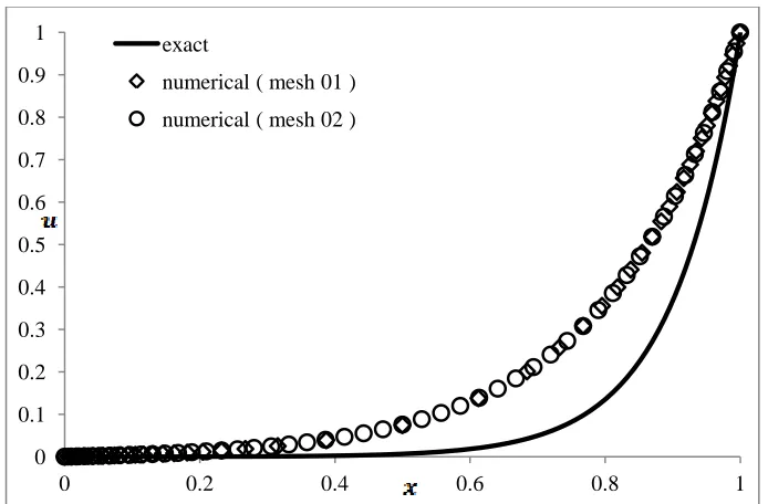
Figure 4.5 Numerical and exact results for Poisson equation (uniform mesh; N = 50; Dirichlet boundaries) ... 56
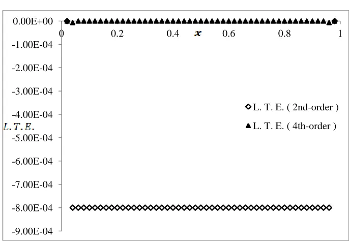
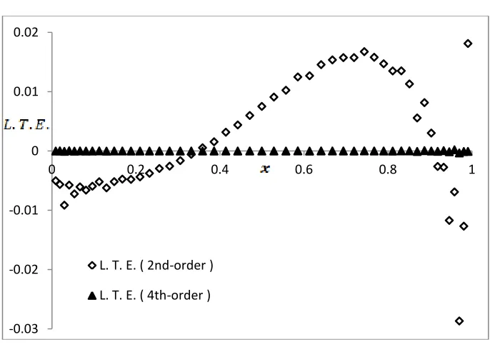
Figure 4.6 Local truncation error for Poisson equation (uniform mesh; N = 50; Dirichlet boundaries; 2nd-order vs. 4th-order scheme) ... 56
Figure 4.7 Numerical and exact results for Poisson equation (uniform mesh; N = 50; west Neumann boundary)... 57
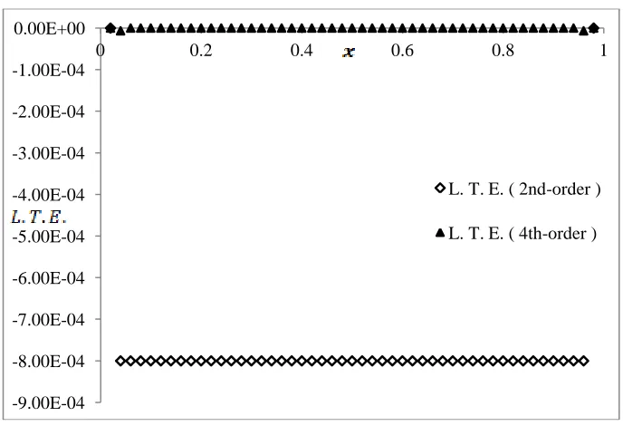
Figure 4.8 Local truncation error for Poisson equation (uniform mesh; N = 50; west Neumann boundary; 2nd-order vs. 4th-order scheme) ... 57
Figure 4.9 Numerical and exact results for Poisson equation (uniform mesh; N = 50; east Neumann boundary)... 58
Figure 4.10 Local truncation error for Poisson equation (uniform mesh; N = 50; east Neumann boundary; 2nd-order vs. 4th-order scheme) ... 58
Figure 4.11 Numerical and exact results for Poisson equation (clustered mesh 01; N = 50; Dirichlet boundaries) ... 59
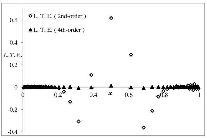
Figure 4.12 Local truncation error for Poisson equation (clustered mesh 01; N = 50; Dirichlet boundaries; 2nd-order vs. 4th-order scheme) ... 59
Figure 4.13 Numerical and exact results for Poisson equation (clustered mesh 02; N = 50; Dirichlet boundaries) ... 60
xiii
Figure 4.15 Numerical and exact results for Poisson equation (clustered mesh 01; N = 50; west Neumann boundary)... 61 Figure 4.16 Local truncation error for Poisson equation (clustered mesh 01; N = 50; west
Neumann boundary; 2nd-order vs. 4th-order scheme) ... 61 Figure 4.17 Numerical and exact results for Poisson equation (clustered mesh 02; N = 50; west
Neumann boundary)... 62 Figure 4.18 Local truncation error for Poisson equation (clustered mesh 02; N = 50; west
Neumann boundary; 2nd-order vs. 4th-order scheme) ... 62 Figure 4.19 Numerical and exact results for Poisson equation (clustered mesh 01; N = 50; east
Neumann boundary)... 63 Figure 4.20 Local truncation error for Poisson equation (clustered mesh 01; N =50; east Neumann
boundary; 2nd-order vs. 4th-order scheme) ... 63 Figure 4.21 Numerical and exact results for Poisson equation (clustered mesh 02; N = 50; east
Neumann boundary)... 64 Figure 4.22 Local truncation error for Poisson equation (clustered mesh 02; N = 50; east Neumann boundary; 2nd-order vs. 4th-order scheme) ... 64 Figure 4.23 Numerical and exact results for steady convection-diffusion equation (uniform mesh;
N = 50; Dirichlet boundaries) ... 66 Figure 4.24 Local truncation error for steady convection-diffusion equation (uniform mesh; N =
50; Dirichlet boundaries; 2nd-order vs. 4th-order scheme) ... 67 Figure 4.25 Numerical and exact results for steady convection-diffusion equation (clustered mesh
01; N = 50; Dirichlet boundaries) ... 67 Figure 4.26 Local truncation error for steady convection-diffusion equation (clustered mesh 01; N
= 50; Dirichlet boundaries; 2nd-order vs. 4th-order scheme)... 68 Figure 4.27 Numerical and exact results for steady convection-diffusion equation (clustered mesh
02; N = 50; Dirichlet boundaries) ... 68 Figure 4.28 Local truncation error for steady convection-diffusion equation (clustered mesh 01; N
= 50; Dirichlet boundaries; 2nd-order vs. 4th-order scheme)... 69 Figure 4.29 Absolute error comparison for adaptive meshing (initial uniform mesh with N = 20;
convection-diffusion equation) ... 71 Figure 4.30 Numerical and exact results for adaptive meshes (initial uniform mesh with N = 20;
xiv
LIST OF ABBREVIATIONS/SYMBOLS
CFD Computational Fluid Dynamics
DIFCA Distance-Function-Based Cartesian
1D One-Dimensional
2D Two-Dimensional
3D Three-Dimensional
PDE Partial Differential Equation
CCFD Cell-Centred Finite Difference
FD Finite Difference
BLK Block
TFDM Traditional Finite Difference Method
ODE Ordinary Differential Equation
MODE Modified Ordinary Differential Equation
FDE Finite Difference Equation
L.T.E. Local Truncation Error
BVP Boundary Value Problem
xv
NOMENCLATURE
φ , u general variables
Sφ,Su source terms
ν viscosity
U reference velocity
L reference length
, , , dimensionless variables
Re Reynolds number
uLB left boundary value
uRB right boundary value
κ thermal conductivity
R diffusion coefficient
a convective speed
x physical coordinate
ξ computational coordinate
B clustering parameter
β coefficient to determine central or backward differencing
ui nodal value at node i
u0 west (left) boundary value
uL east (right) boundary value
xvi
NJ number of cells in blocks J
uJi nodal value at node i in block J
, transformation metrics
BLK J block J
i node or cell number
ci cell centre in cell i
∆xi length of cell i
d diffusion number
C Courant number
Un+1/Un amplification factor
∆t time step
tmax maximum time
xW west node coordinate in the stencil
xP centre node coordinate in the stencil
xE east node coordinate in the stencil
xL left central coordinate in the stencil
xR right central coordinate in the stencil
uL left central value in the stencil
uR right central value in the stencil
uW west nodal value in the stencil
uE east nodal value in the stencil
1
CHAPTER 1
INTRODUCTION
1.1 Background
Generally, for Computational Fluid Dynamics (CFD), there are three types of mesh-based
discretisation methods: Finite Difference, Finite Volume and Finite Element. Each
method has their strengths and weaknesses. Among these methods, Finite Difference is
the most efficient and, since it is a relatively straightforward method, it is often used in
developing numerical formulations to deal with initial and boundary value problems.
Another strength of the finite difference method is that Taylor series expansion can be
easily applied to analyze local truncation errors. This property can be exploited to analyze
the accuracy of the solution. But there is an important limitation in applying the finite
difference method, which is the requirement of a structured grid. Therefore, the method
cannot easily be applied on complex domains, making the finite difference method
unpopular in commercial CFD software. However, since the finite volume and finite
element methods are also not without restrictions, some researchers have preferred to
improve the traditional finite difference method to make it useful for a wider range of
applications. This has led to the development of structured grid generation techniques,
algorithms for solution of the governing equations in curvilinear coordinates and
multi-block methods. The fundamental concepts of the finite difference and finite volume
methods are explained in details in many CFD books, eg., Hoffmann and Chiang[1], Ramshaw[2], Lomax et al.[3], Anderson et al.[4], Roache[5], Anderson[6], Versteeg and Malalasekera[7], Ferziger and Peric[8], Chung[9] and Patankar[10].
The general convection-diffusion equation is often used to study the utility of new
algorithms for the Navier-Stokes equations (eg. see [7, 8, 10]). The convection-diffusion
equation is also popular for the study of some specific issues in numerical schemes, such
as Kalita’s[11] study on the effects of clustering on simulations, the significance of “wiggles” in the numerical results by Gresho and Lee[12]
, Thiart’s[13] research on solving fluid flow and heat transfer problems on non-staggered grids, and the work of Date[14] on collocated variables for unstructured meshes. A variety of new methods have been
2
complex meshes easier. For example, Chai and Yap[15] developed a distance-function-based Cartesian (DIFCA) grid finite volume method for irregular geometries and applied
the algorithm on the convection-diffusion equation. A mesh-free finite difference method
based on the Poisson equation has been developed by Seibold[16].
Due to the significant commonalities among the governing equations of the flow of a
Newtonian fluid, such as the continuity equation, momentum equations and energy
equation, it is convenient to introduce a general variable φ to express the conservative
form of these equations. The general conservative form of the convection-diffusion
equation can be written as
. (1.1)
Equation (1.1) is the general transport equation for incompressible flow. Property φ can
stand for velocity components, temperature or some other variable in physical problems.
To be precise, if φ equals to 1, Γ = 0 and Sφ = 0, equation (1.1) is the mass conservation
equation; if φ equals to u, Γ = ν (viscosity) and , equation (1.1) is the x
-momentum equation; if φ equal to , Γ = ν and , equation (1.1) is y
-momentum equation; if φ equal to w, Γ = ν and , equation (1.1) is z
-momentum equation; if φ equal to et, Γ = κρ and
, equation (1.1) is
the energy equation.
Equation (1.1) also clearly emphasizes the physical background in fluid mechanics for
transport processes: (rate of increase of φ in the fluid element) + (net rate of flow of φ out
of the fluid element) + (rate of increase of φ due to diffusion) = (rate of increase of φ due
to sources).
1.2 One-dimensional Models
The focus in this thesis is the development of a new generalized finite difference
methodology. This new approach is explained and subsequently validated using
one-dimensional mathematical models. The following examples illustrate how these model
equations are obtained from the transport equation (1.1) and are representative of the
3
Example 1.Nondimensional 1D Transport Equation
If the general transport equation is used to express the x-momentum equation, equation
(1.1) becomes
. (1.2)
Re-arranging equation (1.2) using differentiation rules,
. (1.3)
Due to the conservation of mass, = 0. Therefore, equation (1.3) is
. (1.4)
The one-dimensional (1D) version of this equation is
. (1.5)
The numerical modeling of equation (1.5) is simplified if it is expressed in
nondimensional form. Generally, there are three major advantages in
nondimensionalization: reduce the total number of parameters; nondimensionalized
parameters have a more transparent meaning; parameters and variables can be rescaled to
make the computed quantities have relatively similar magnitudes[17]. Furthermore, the nondimensional transport equation can be applied to problems with the same boundary
conditions for different cases and the results from these cases can be easily compared.
For nondimensionalization, a set of dimensionless variables needs to be defined.
Define reference velocity magnitude U, length L, and dimensionless variables , , ,
by , , , . Substituting these expressions into equation (1.5),
the nondimensional x-momentum equation in 1D is the convection-diffusion equation
(1.6)
where is the velocity, is the Reynolds number, is the pressure gradient
4
This transport equation is classified as a non-linear partial differential equation (PDE)
since it includes a product of the dependent variable and its derivative.
Example 2. Linear 1D Initial Value Problem/ Boundary Value Problem
A model linear PDE is obtained by assuming that the convective speed, which is the
coefficient of the term, is constant. Combining the pressure gradient with the source
term in (1.5), the 1D linear transport equation becomes
(1.7)
where a is the constant convective velocity. Let us consider equation (1.7) on
with initial and boundary conditions , and
respectively. Here uLB and uRB are constant values. Figure 1.1 shows the physical domain
and the imposed boundary conditions.
Figure 1.1 Boundary conditions and domain in 1D
Define dimensionless variables
, ,
, , , where
. Note that , is mapped to and is mapped to .
Using , substitute u into equation (1.7) to obtain the nondimensional
PDE
(1.8) where is the constant wave speed,
is called the “diffusion” coefficient and the nondimensionalized domain becomes a unit domain, .
The initial condition becomes , which can be re-arranged to give
5
Similarly, the nondimensional boundary conditions become
and (1.10)
Example 3. 1D Heat Conduction in a Solid Material
Using the nondimensional partial differential equation (1.8), take .
Then the governing heat conduction equation is written as
(1.11)
where κ is the thermal conductivity.
1.3 Classification of Model Equations
The above three examples show how the general transport equation can be
nondimensionalized, and how the nondimensional transport equation corresponds to
specific mathematical models. These second-order PDEs can be further classified. The
classification is crucial when deciding how to discretize these second-order PDEs so that
the physics of the phenomenon is properly modeled. Clarifying the different types of
PDEs is also beneficial since different forms of boundary and initial conditions are
required to formulate the problems with different types of PDEs.
Dropping the bars from the notation for convenience, the 1D nondimensional transport
equation (1.8) becomes
. (1.12)
a. If the value for D goes to infinity, the diffusion term drops out and the equation
becomes the hyperbolic equation
. (1.13)
From a geometric interpretation, there are two real characteristic curves for a hyperbolic
PDE. Two initial conditions and two boundary conditions restrict the solution domain,
which is a conic section. In fluid mechanics problems, when the Reynolds number
becomes quite high, the solution is dominated by the convection terms. For hyperbolic
6
b. If the value for a, which is the coefficient of the convection term, equals to 0, the
equation is the parabolic equation
. (1.14)
From a geometrical aspect, only one characteristic curve exists for a parabolic equation.
The solution domain will be an open region. The solution forms from the initial plane of
data to downstream within the domain, propagating forward in time, meanwhile restricted
by the specified boundary conditions [1].
c. The third classification is elliptic equation. For an elliptic PDE, the characteristic
curves are imaginary. Any disturbance propagates to every direction in the region at
infinite speed. The solution domain is a closed region [1]. Elliptic equations, which describe equilibrium phenomena, can be divided into two groups: Poisson equation and
convection-diffusion equation. Setting a = 0, and taking steady conditions, equation (1.8)
becomes the Poisson equation
(1.15)
Otherwise, the elliptic equation is the steady convection-diffusion equation
(1.16)
1.4 Clustering Functions
Mesh quality is an important consideration for all mesh-based numerical simulation
methods. If the solution is smooth with small gradients, a uniform mesh will usually
suffice. However, if the solution undergoes large gradients, such as in boundary layer
flows on no-slip walls, the mesh must be appropriately designed. This usually entails
creating a mesh with variable spacing, perhaps small spacing close to the physical
boundary and larger spacing further away from the boundary. These grids are referred to
as clustered or stretched grids.
The new generalized finite difference method developed in this thesis is designed to
easily handle arbitrary grid spacing without any knowledge of the clustering functions
used to generate the mesh or, in fact, for nodes that are randomly placed without using
7
finite difference method and the proposed method, the following two clustering functions
have been used in this thesis:
(1.17)
and
(1.18)
Both of these functions map into , with clustering at x = 0 and x = 1.
The mesh obtained from equation (1.17) is referred to as mesh 01 in Chapter 2; the mesh
generated from equation (1.18) is called mesh 02. The parameter in (1.17) is related to
the number of nodes in the mesh, = 0.5(M + 1) where M is the number of nodes in the
mesh including endpoints. The parameter B in equation (1.18) must satisfy the condition
1 < B < 2. B controls the degree of clustering, with more clustering of the nodes near x =
0 and x = 1 as B 1.
1.5 Research Objectives
The objective of this research is to develop a new generalized finite difference method
which can be used to solve any PDE in an arbitrarily discretized domain. Although this
research is focused only on one-dimensional (1D) problems, it is essential to guarantee
that the new method can be applied effectively in 2D and 3D without any potential
problems. The development of the algorithm starts by considering the general
convection-diffusion equation since it is a model for many physical phenomena
encountered in engineering and science. The 1D formulation is easy to derive and the
code programming is not as complicated as the 2D or 3D cases. Finding the potential
problems in a 1D model and resolving them in a manner that can be extended to higher
dimensions can ensure applicability in 2D or 3D.
Two types of finite difference schemes are formulated and analyzed, the Cell-Centred
Finite Difference (CCFD) method and the Stencil Mapping method. The research begins
8
several cases, our research has identified the interpolation scheme as the source of this
inaccuracy. Lakner and Plazl[20] proposed a symbolic-numerical solution procedure based on the finite difference method to solve PDEs on irregular domains. Their concept uses
the theory of splines to develop appropriate interpolation schemes, which we have also
taken into consideration for the CCFD method. However, although the interpolation
problem can be solved by applying the theory of splines [21], it is time-consuming for computer calculation and cannot be easily applied in 2D and 3D. Thus, the research is
re-directed to the development of a new generalized finite difference method which we refer
to as the Stencil Mapping method. Spotz[22] showed that knowing the mapping derivatives is especially meaningful to the accuracy of the finite difference method. In the
proposed Stencil Mapping method, each difference stencil is mapped individually to a
generic computational stencil, rather than the entire physical domain being mapped to a
computational domain. This is accomplished using a quadratic mapping function, from
which the mapping derivatives can be analytically determined.
In this thesis, the proposed Stencil Mapping method is also applied to the development of
4th-order accurate finite difference schemes. High order finite difference schemes usually require non-compact stencils, which use grid points that are not adjacent to the node at
which the differencing equations are applied. For example, Castillo et al.[23][24] developed mimetic and support-operator differencing methods for 4th-order schemes on a non-compact stencil. However, non-non-compact differencing schemes for higher-order accuracy
always need special treatment for nodes near boundaries. Therefore, it is desirable to
develop a compact stencil algorithm for higher-order schemes. The compact stencil
algorithm only uses the two nodes adjacent to the node at which the differencing equation
is formulated. In this way, no special equation is needed when applying the discretisation
equation on the nodes near boundaries. Some researchers have worked on developing
9
applied on schemes that are more accurate than 4th-order, such as 8th-order, and the same 3-point compact stencil can be preserved.
1.6 Thesis Layout
In this research, a computer code has been written for the finite difference method in C
programming language, in order to compare the convenience of the proposed schemes
from either the formulation or implementation aspect, and to assess the accuracy of the
results.
Chapter 2 covers details of the traditional finite difference method, focusing mainly on
formulations, how it is implemented in a code, where the complexity is when dealing
with a multi-block and clustered meshes and the accuracy of numerical results compared
with the exact results.
Chapter 3 discusses a recently proposed finite difference method called Cell-Centred
Finite Difference (CCFD). The algorithm is developed for the general
convection-diffusion equation. Three types of interpolation – averaging, shifting and differencing, are
formulated. Consistency is investigated for the steady convection-diffusion equation and
stability is analyzed for the unsteady equation.
Chapter 4 provides the formulation for the new Stencil Mapping method in 1D for the
general convection-diffusion equation, applying both 2nd-order and 4th-order differencing schemes. The algorithm is implemented with either Dirichlet or Neumann boundary
conditions on either a uniform mesh or clustered mesh to determine if the new scheme is
applicable and if the results are accurate. The local truncation error is used to test the
10
CHAPTER 2
TRADITIONAL FINITE DIFFERENCE METHOD
As indicated in the introductory chapter, the convection-diffusion equation is often used
to analyze new numerical methods for partial differential equations. In this chapter the
1D form of the steady convection-diffusion equation,
(2.1)
is used to discuss the traditional implementation of the Finite Difference (FD) method.
This is equation (1.16) with R = aD and S redefined. Since the FD method is well-known,
the emphasis in this chapter is to highlight the key issues that make the method more
complicated when applied to complex geometries.
In the Finite Difference methodology, the derivatives are approximated by finite
differences, and the differential equation (2.1) is applied at each node in the discretised
domain. Several types of 1D mesh, with different size of cells, are tested in this thesis.
These mesh types, chosen because they are commonly used for finite difference CFD
simulations in complex domains, are known as uniform, clustered and multi-block. After
discussing the developments related to these mesh features, results from the various
schemes are presented at the end of the chapter.
2.1 Uniform Mesh
To illustrate the basic FD method, consider the solution of the convection-diffusion
equation (2.1) on a 1D domain with five cells, as shown in Fig. 2.1. The domain length is
1 unit, with five cells in the domain, with four internal nodes and two boundary nodes.
Since the grid spacing is equal, the length of each cell is Δx = 1/5. For Dirichlet boundary
conditions, the west (left) boundary is set to be 0, and the east (right) boundary is set to
be 1. As shown in Chapter 1, any Dirichlet boundary value problem associated with the
11
Figure 2.1 Single block 1D uniform mesh with five cells
The second-order accurate central differencing formula is used to approximate the
diffusion term in equation (2.1), and either the second-order central differencing or
first-order backward differencing scheme is applied for the convection term (assuming R > 0).
The discretisation equation is
(2.2)
where index i refers to any node in the domain, i-1 refers to the left-side node of node i
and i+1 refers to the right-side node of node i. If β = 0, central differencing is applied for
the convection term, while β = 1 corresponds to backward differencing.
After applying the discretisation equation (2.2) at every internal node, four coupled linear
algebraic equations with four unknowns can be formed. The difference equation (2.2) can
be re-arranged as
. (2.3)
Since the node numbers start from 1 and end at 6, u1 and u6 are the west and east
boundary conditions, respectively, i.e., u1 = 0 and u6 = 1. Interior nodes run from node
numbers 2 to 5.
Therefore, at i = 2:
(2.4)
At i = 3:
(2.5)
At i = 4:
(2.6)
At i = 5:
12
Since u1 and u6 are boundary nodes, their values are already known. Equations (2.4),
(2.5), (2.6) and (2.7) can be written as a system of linear algebraic equations
(2.8)
The value for β is set to 0 or 1, depending whether central differencing or backward
differencing is chosen for discretisation of the convection term. Then, this tri-diagonal
matrix equation (2.8) can be solved by applying Thomas’ Algorithm [1]
to obtain the
results for all nodal values.
In general, suppose the uniform mesh has N cells, which means the mesh has (N-1)
interior nodes. Applying difference equation (2.3) at each node leads to an (N-1)⨯(N-1)
tri-diagonal matrix equation which can be expressed as
.
2.2 Multi-block Mesh
In order to use the Finite Difference method for complex domains, the multi-block
technique is often implemented. For multi-block mesh problems, the domain is divided
into several blocks. Each block (BLK) is then meshed with a structured grid. For
purposes of the present discussion, and without loss of generality, the cells inside every
block are assumed to be uniform, but the cells in one block can be different from the cells
in other blocks. When solving multi-block problems, the key question is about how to
deal with the block interfaces. Accurate inter-block communication is essential. The
problem of transferring accurate information across block interfaces adds significantly to
the complexity of the traditional FD method (TFDM) for practical applications. This is
one of the motivations in the current research to develop a new finite difference method
that can easily handle block interfaces. In this section, two methods to solve the interface
13
Figure 2.2 illustrates an example of a multi-block mesh, which has four blocks. This
example will be used in the explanation of inter-block communication schemes.
Figure 2.2 1D 4-block mesh
The convection-diffusion equation (2.1) is applied on this 4-block mesh. The domain and
the boundary conditions are the same as in section 2.1. The length of the cells in each
block is denoted as ∆x1, ∆x2, ∆x3 and ∆x4 for BLK 1, BLK 2, BLK 3 and BLK 4,
respectively. The number of cells in BLK i is denoted as Ni.
2.2.1 Method A
Method A deals with the evaluation of the interface nodes by introducing “ghost” or
imaginary nodes and using an overlapping procedure. In this 4-block case, there are three
interfaces, but four imaginary nodes should be taken into consideration to implement this
overlapping method. To simplify the discussion, solution values in BLK J are denoted by
uJ. The detailed iterative procedure is as follows:
i. Initialize imaginary nodal values. Since there are three interfaces, there should be three
initialized imaginary nodal values, which are regarded as the east end nodes of BLK 1,
BLK 2 and BLK 3. These three imaginary nodes are placed so as to preserve the
uniformity in each block, and the value at these nodes is denoted as u1N1+2, u2N2+2 and u3N3+2, respectively. These “ghost” nodes are shown in Fig. 2.3.
14
ii. After initializing the value for u1N1+2, the east boundary condition (at N1+2) for BLK 1
is considered to be known. The west boundary condition for BLK 1 is the west boundary
condition of the domain. Applying the discretisation equation at every interior node of
BLK 1, nodal values on BLK 1 can be calculated by solving the resulting (N1-1)⨯(N1-1)
tri-diagonal matrix.
iii. From step ii, the first interface node value u1N1+1, which is also u21, is known. Since
the nodal value u2N2+2 has already been initialized, the west boundary condition is u21
and the east boundary condition is u2N2+2 for BLK 2. Apply the difference equation (2.3)
at every node in BLK 2, from which all nodal values in BLK 2 can be calculated.
iv. Apply the same procedure as in step iii to calculate all nodal values for BLK 3,
including the interface node between BLK 3 and BLK 4.
v. The last block in the domain, which is BLK 4, contains the east boundary condition (at
N4+1) of the domain. Thus, the east boundary condition for BLK 4 is known, which is
u4N4+1. The west boundary condition for BLK 4 is u40 at the fourth imaginary node,
which is located on BLK 3 as shown in Fig. 2.3. Find the two neighbour nodes of the
imaginary west boundary node located in BLK 3. The solution at these two neighbour
nodes can be expressed as u3i and u3i+1, and the locations are x3i and x3i+1. The location
for u40 is denoted as x40. Apply distance-weighted average to obtain the value for u40 as
. (2.9)
Therefore, the west boundary condition for BLK 4 is known. Apply the discretised
equation (2.3) on every interior node in BLK 4. Solving the tri-diagonal matrix, the nodal
values for BLK 4 can be obtained.
vi. After solving for all the nodal values in BLK 4, the value u3N3+2 at imaginary node x3N3+2 needs to be updated. Find the two neighbour nodes adjacent to node x3N3+2 in BLK
4. The notations for the values at these two nodes are u4i and u4i+1, and the locations of
these two nodes are x4i and x4i+1. Use distance-weighted average to obtain the updated
15
. (2.10)
vii. Repeat similar calculations as in step iv in BLK 3 to update the nodal value for
u2N2+2. Then perform similar calculations as in step iii to update the nodal value for u1N2+2. To complete this iteration, carry out similar calculations as in step ii to update the
nodal values on BLK 1.
viii. Repeat the calculations from step ii to vii to iteratively update the nodal values in the
domain until the values for u1N1+1, u2N2+1 and u3N3+1 converge to within the
user-specified tolerance.
2.2.2 Method B
The same setup as shown in Fig. 2.3 is used to illustrate this method. Method A connects
the blocks through imaginary nodes overlapping at each interface during the calculations.
For Method B, the connection is at the interface node itself. Assume that the derivative of
the solution from the west side of the interface node is the same as the derivative from the
east side of the interface node, i.e., assume that the solution is differentiable at the
interface node. This condition can be expressed as
(2.11)
where – represents west and + represents east.
For example, taking BLK 1 and BLK 2, and using one-sided difference approximations
for the derivatives in equation (2.11) gives
(2.12)
. (2.13)
The interface node is the last node in BLK 1, but also the first node in BLK 2. Thus,
. (2.14)
Substituting equations (2.12), (2.13), (2.14) into equation (2.11) yields
. (2.15)
16
Considering the example illustrated in Fig. 2.3, the solution procedure is as follows:
i. Initialize the three nodal values u22, u32 and u42.
ii. Using the discretisation equation (2.3), set up the matrix system for BLK 1 similar to
that in equation (2.8) and calculate the nodal values in BLK 1.
iii. Using similar equations as (2.12), (2.13), (2.14) and (2.15), calculate the nodal values
for BLK 2 and BLK 3.
iv. After step iii, the nodal value for the third interface node u3N3+1, which is also the
nodal value for u41, is known. Since the east boundary condition for the domain is
already known, which is u4N4+1, the discretised equation (2.3) can be applied at every
node in BLK 4. The nodal values for BLK 4 can be calculated by solving the tri-diagonal
matrix.
v. From step iv, the updated nodal value for u42 is available. Repeat the calculation from
step ii to iv, until the nodal values u22, u32 and u42 converge to within the user-specified
tolerance.
2.3 Clustered Mesh
In a clustered mesh, the length of the cells is different from each other. In the TFDM, the
approach is to map the non-uniform mesh to a uniform one. Figure 2.4 demonstrates this
mapping approach. The domain 0 ≤ x ≤ 1 is mapped to 0 ≤ ξ ≤ 1, with the same number
of cells. This mapping of the domain can be expressed by a mapping function,
. (2.16)
The TFDM needs to be applied in the ξ system, where the nodes are uniformly
distributed. As illustrated in Fig. 2.4, the length of every mesh cell in the ξ system is ∆ξ =
1/N, where N represents the number of cells. To apply the standard finite difference
formulae in this mapping approach, the governing differential equation must be
transformed into the ξ system. Using chain rules, the terms in the convection-diffusion
equation (2.1) transform as
(2.17)
17
Figure 2.4 Mapping a 1D non-uniform mesh to a uniform mesh
Using equations (2.17), the governing differential equation (2.1) transforms to
(2.18)
If the transformation function (2.16) is known analytically, such as the functions defined
by equations (1.17) and (1.18), the metrics and can be evaluated exactly at all
nodes. If the clustered mesh is obtained from grid generation equations, the metrics are
approximated at any node, which is denoted by i in the ξ system, as
(2.19)
. (2.20)
Applying three-point central differencing to approximate the diffusion term and
backward differencing to approximate the convection term, equation (2.18) is discretized
as
(2.21)
which can be re-arranged as
(2.22)
After substituting equation (2.19) and (2.20) into (2.22), since the location of each node
in the x-coordinate system is known, a system of linear algebraic equations can be
derived. Taking the mesh in Fig. 2.4 as an example, there are N+1 nodes in the domain.
18
respectively. Thus, after applying discretised equation (2.22) at every node in the domain, an (N-1)⨯(N-1) matrix system can be set up. Every nodal value in the domain can be
evaluated by solving this matrix system.
2.4 Examples
In the following examples, the solution domain is from 0 to 1, the west boundary
condition is 0 and the east boundary condition is 1.
2.4.1 Uniform Mesh
The uniform mesh is the simplest of all meshes, and forms the basis for the TFDM. This
is primarily due to the fact that the classical finite difference formulae used to
approximate derivatives lose at least one order of accuracy if the spacing is non-uniform.
2.4.1.1 Laplace Equation
The Laplace equation, obtained by setting R = 0 and S = 0 in equation (2.1), i.e.
(2.23)
is solved on a uniform mesh by applying the traditional finite difference method. The
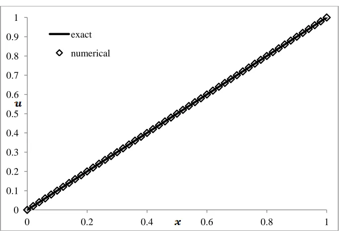
number of cells is 40. Figure 2.5 shows the comparison between numerical results from
the code and the exact solution, given by u(x) = x. The numerical results are identical to
the exact results.
Figure 2.5 Comparison of exact and TFDM solutions of Laplace equation (uniform mesh; N = 40) 0
0.1 0.2 0.3 0.4 0.5 0.6 0.7 0.8 0.9 1
0 0.2 0.4 0.6 0.8 1
19
2.4.1.2 Convection-Diffusion Equation
In this section, the homogeneous convection-diffusion equation
(2.24)
is solved on a uniform mesh by applying the traditional finite difference method. The
exact solution of the boundaryvalue problem is
. (2.25)
Figure 2.6 shows the comparison between the numerical results and the exact solution.
The number of cells used for the simulation is 40. Central differencing is applied to the
diffusion term, backward differencing is applied on the convection term, and R is set to
10.
As illustrated in Fig. 2.6, there are some differences between the numerical results and
the exact solution. The largest absolute error has the value 0.042 and occurs at node 37.
Figure 2.6 Comparison of exact and TFDM solutions of steady convection-diffusion equation (uniform mesh; N = 40; R = 10)
2.4.2 Multi-block Mesh
Consider the 4-block mesh on the interval [0,1] illustrated in Fig. 2.3. Boundary
conditions are 0 for the west boundary and 1 for the east boundary. Block interfaces are
0 0.1 0.2 0.3 0.4 0.5 0.6 0.7 0.8 0.9 1
0 0.2 0.4 0.6 0.8 1
20
at x equal to 0.1, 0.4 and 0.8. The numbers of cells in each block are 8, 5, 5 and 5 for
BLK 1, BLK 2, BLK 3 and BLK 4, respectively. The convergence tolerance is set to be
10-6. After running the code using both Method A and Method B to deal with the interface problem, it was determined that Method A provides a better solution for both
the Laplace equation and convection-diffusion equation. Therefore, only the results from
Method A are shown for the following cases.
2.4.2.1 Laplace Equation
The Laplace equation (2.23) is solved on the 4-block mesh by applying the traditional
finite difference method. Figure 2.7 illustrates the results from the numerical calculation
and the exact solution. The numerical results are not exactly the same as the exact
solution, but the largest absolute error is only 8.75x10⁻⁶, occurring at node 14.
Figure 2.7 Comparison of exact and TFDM solutions of Laplace equation (4-block mesh; N = 24)
2.4.2.2 Convection-Diffusion Equation
The convection-diffusion equation (2.24) is solved on the same 4-block mesh by applying
the TFDM with central differencing for the diffusion term and backward differencing for
the convection term.
0 0.1 0.2 0.3 0.4 0.5 0.6 0.7 0.8 0.9 1
0 0.2 0.4 0.6 0.8 1
21
Figure 2.8 shows the comparison between the numerical calculation and the exact
solution. The largest absolute error appears at node 21, with a value of 0.089. The
solution of the convection-diffusion equation is not as accurate as the Laplace equation,
but one should note that the discretization of the Laplace equation is fully second order,
while the discretization of the convection-diffusion equation uses first order upwinding
for the convective term.
Figure 2.8 Comparison of exact and TFDM solutions of steady convection-diffusion equation (4-block mesh; N = 24; R = 10)
2.4.3 Clustered Mesh
The mesh is clustered at both ends, based on the clustering functions defined by
equations (1.17) and (1.18). For clustered mesh 01, the function is arcsinh. For clustered
mesh 02, the function is Ln with B = 1.2.
2.4.3.1 Laplace Equation
The solution of the Laplace equation (2.23) is illustrated in Fig. 2.9, showing the
comparison between the numerical and exact solutions. The numerical results do not
agree with the exact solution. For the clustered mesh 01, the largest absolute error is
0.349, which appears at node 31. The largest absolute error appears at node 30 for the
0 0.1 0.2 0.3 0.4 0.5 0.6 0.7 0.8 0.9 1
0 0.2 0.4 0.6 0.8 1
22
clustered mesh 02, with a value of 0.099. The TFDM does not predict the correct solution
on these clustered meshes.
Figure 2.9 Comparison of exact and TFDM solutions of Laplace equation (clustered mesh; N = 50)
2.4.3.2 Convection-Diffusion Equation
The convection-diffusion equation (2.24) is solved on the same clustered meshes by
applying the TFDM with central differencing scheme applied to the diffusion term and
backward differencing for the convection term. R is set to be 10.
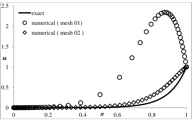
Figure 2.10 shows the comparison between the numerical calculation and exact solution.
The numerical results are not accurate compared to the exact solution, especially for
mesh 01. The largest absolute error is 2.08 at node 34 and 0.233 at node 43, for clustered
mesh 01 and 02, respectively. Certainly, the number of nodes in the mesh will influence the solution accuracy, but refining the mesh does not always resolve the accuracy issue.
0 0.2 0.4 0.6 0.8 1 1.2
0 0.2 0.4 0.6 0.8 1
exact
23
Figure 2.10 Comparison of exact and TFDM solutions of steady convection-diffusion equation (clustered mesh; N = 50; R = 10)
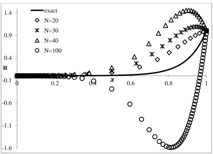
Figure 2.11 below shows the results from TFDM solutions on clustered meshes with
different number of cells. These mesh files were generated based on the arcsinh function
defined by equation (1.17). As shown in this figure, increasing the number of cells does
not produce more accurate results in this particular example. In fact, the numerical results
become worse as the number of grid points increases, even becoming negative for large
N. This example confirms that clustered meshes can produce erroneous results if they are
not properly designed, requiring considerable expertise on the part of the user.
0 0.5 1 1.5 2 2.5
0 0.2 0.4 0.6 0.8 1
exact
24
Figure 2.11 Comparison of exact and TFDM solutions of steady convection-diffusion equation on meshes with different number of cells (clustered mesh; R = 10)
The logarithmic function defined in equation (1.18) was used to create two clustered
meshes with different values of B. Recall that 1 < B < 2 and the mesh becomes more
clustered for B closer to 1. Results from the solutions on these two meshes are compared
in Fig. 2.12. It is obvious that the results are more accurate with the higher value of B,
which means the mesh is more uniform. This comparison demonstrates that the degree of
clustering has an effect on the solution accuracy, as has been pointed out by Kalita[11] and others.
-1.6 -1.1 -0.6 -0.1 0.4 0.9 1.4
0 0.2 0.4 0.6 0.8 1
25
Figure 2.12 Comparison of exact and TFDM solutions of steady convection-diffusion equation (clustered mesh with B = 1.2 and B = 1.75; N = 50; R = 10)
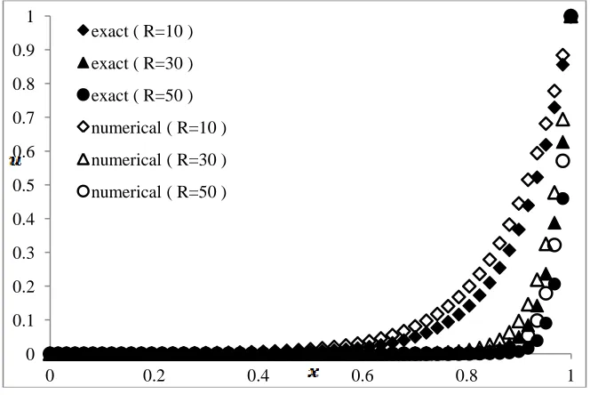
Figure 2.13 illustrates the results from the solutions with different values for R. The
clustered meshes are based on the function (1.18) with the same value for B = 1.75. The
largest absolute error becomes higher when the value of R increases, with the value 0.077
at node 45, 0.09 at node 49 and 0.11 at node 50, respectively. These larger errors can be
attributed to the higher gradients near the east boundary for larger R.
Figure 2.13 Comparison of exact and TFDM solutions of steady convection-diffusion equation (clustered mesh 02 with B = 1.75; N = 50; R = 10, 30, 50)
0 0.1 0.2 0.3 0.4 0.5 0.6 0.7 0.8 0.9 1
0 0.2 0.4 0.6 0.8 1
exact
numerical ( B=1.2) numerical ( B=1.75 )
0 0.1 0.2 0.3 0.4 0.5 0.6 0.7 0.8 0.9 1
0 0.2 0.4 0.6 0.8 1
26
2.5 Summary
The traditional finite difference method can be used to accurately solve the Laplace
equation on either a uniform mesh or a multi-block mesh. For steady
convection-diffusion, although the results are not as accurate as the results for the Laplace equation,
the error can still be kept small. Multi-block implementation is complicated due to the
inter-block communication. The method to deal with the interface problem needs to be
applied cautiously; otherwise, it may cause trouble in the programming and the accuracy.
Applying the TFDM on a clustered mesh must also be done with care, since the results
depend significantly on the functions used to generate the clustered mesh. One of the
reasons for this is, in the TFDM, only one mapping function is applied to map the whole
clustered mesh into a uniform mesh. The metrics are approximated based on the same
mapping function, which is not always accurate for all cases, and this accuracy will affect
the numerical results. Due to these reasons, a Cell-Centred Finite Difference Method, for
which no mapping is needed when dealing with multi-block and clustered meshes, is
27
CHAPTER 3
CELL-CENTRED FINITE DIFFERENCE METHOD
Although the traditional finite difference method has been applied very successfully for
many CFD applications, it has some weaknesses such as those illustrated in Chapter 2.
The strengths of the method, in particular its simplicity in development and
programming, are lost if one is interested in solving flows in very complex geometries.
The main restriction that limits the applicability of the traditional finite difference method
is that it cannot handle arbitrary mesh topologies. Since complicated flow domains are
more easily meshed using arbitrary polygonal (2D) or polyhedral (3D) elements, the CFD
community generally regards the finite difference method as non-applicable for industrial
problems. For this reason, most commercial CFD codes are based on either the Finite
Volume method or the Finite Element method, e.g., ANSYS Fluent[28], STAR-CCM+[29], CONVERGE[30], FLOW-3D[31] and COMSOL[32].
In an attempt to devise a finite difference scheme that can be implemented on an arbitrary
mesh, Salih[18] and Situ[19] introduced the Cell-Centred Finite Difference (CCFD) method. In the CCFD method, the differential equation is approximated at the centre of each
(arbitrary) cell in the domain by placing a local coordinate system at the cell centroid and
aligning it with the global Cartesian coordinate system, with the local stencil arms cutting
the edges of the cell, as shown in Fig. 3.1. The method derives its strength from the fact
that the differencing stencil is confined to the cell. Instead of assembling a matrix system
as in the traditional node-based finite difference method, a point-wise iterative approach
is used in CCFD to determine the solution at all cell centres. Nodal values are then
obtained by interpolation of the cell-centre values. Research by Salih[18] and Situ[19] focused mainly on implementation issues for 2D elliptic (Laplace) and parabolic
(unsteady heat conduction) PDEs. Their simulations demonstrated that the CCFD method
can handle triangulated domains as well as uniform and clustered Cartesian grids.
However, there were some issues with accuracy for convection-diffusion equations,
28
Figure 3.1 Cell-Centred stencils in an arbitrary 2D mesh
This chapter is devoted to a fundamental analysis of the CCFD method. In particular, the
main source of inaccuracy due to numerical modeling errors is identified and some
simple procedures to alleviate the problem are proposed. This analysis is carried out for
the 1D model problems discussed in Chapter 1.
3.1 General 1D CCFD Formulation
In the Cell-Centred Finite Difference method, the differencing stencil is kept within each
cell. Therefore, whether the mesh is uniform or not does not affect how the method
works. The discretized equations are valid for every cell in the domain. Take an arbitrary
1D mesh and consider the general unsteady convection-diffusion equation (1.12). Figure
3.2 shows two cells in the arbitrary mesh with cell-centres and nodes denoted as ci-1 and
ci, and as i-1, i and i+1 respectively.
Figure 3.2 Two adjacent cells in a 1D arbitrary mesh
Applying three-point central differencing on cell-centres for the diffusion term and
backward differencing on the convection term, the discretized form of equation (1.12) at
any cell-centre ci is:
29
Implementation of the CCFD method proceeds as follows:
Step 1: Make an initial guess for the solution at all internal nodes.
Step 2: Use discretisation equation (3.1) to determine the values at the cell-centres.
Step 3: Use distance-weighted averaging to update the nodal values, i.e., for each i,
. (3.2)
Then repeat the second and third steps until the differences for the nodal values between
two successive iterations converge to within the specified tolerance.
Both the multi-block mesh and the clustered mesh problems can be solved based on the
same procedures as for the uniform mesh. For the multi-block mesh, the interface nodes
do not cause any complexity. For the clustered mesh, a mapping is no longer required to
evaluate the nodal values. The procedures for CCFD calculations are much simpler, and
programming the code is much more straightforward to accomplish. In brief, this CCFD
method is much easier to implement compared with the traditional finite difference
method.
3.2 Examples for Steady Equations
3.2.1 Uniform Mesh
For the following examples, the domain is of unit length, with west and east boundary
conditions as 0 and 1, respectively. The number of cells in the domain is 50.
3.2.1.1 Laplace Equation
The Laplace equation (2.23) is solved on a uniform mesh by applying the above steps for
the Cell-Centred Finite Difference method. Figure 3.3 shows the comparison between the
numerical results from the code and the exact results. The numerical results perfectly
30
Figure 3.3 Comparison of exact and CCFD solutions of the Laplace equation (uniform mesh; N = 50; averaging method)
3.2.1.2 Steady Convection-Diffusion Equation
Consider the steady convection-diffusion equation (2.1) with R = 10 and S = 0. Second
order central differencing is applied for the diffusion term and backward differencing is
applied for convection term. Figure 3.4 shows the comparison between numerical results
from the code and the exact solution given by equation (2.25).
As illustrated in Fig. 3.4, there are some significant differences between the numerical
results and the exact results. The largest absolute error appears at node 44, with a value of
0.246. This corresponds to a large relative error of 1.0. This result is analyzed in section
3.3 below.
0 0.1 0.2 0.3 0.4 0.5 0.6 0.7 0.8 0.9 1
0 0.2 0.4 0.6 0.8 1
31
Figure 3.4 Comparison of exact and CCFD solutions of convection-diffusion equation (uniform mesh; N = 50; averaging method)
3.2.2 Clustered Mesh
The clustered meshes are generated from a separate code, using the functions defined in
equations (1.17) and (1.18) to build the mesh files 01 and 02 as described in Chapter 1.
The number of cells in each mesh is 50 and the domain has unit length. Boundary
conditions are 0 and 1 at west and east, respectively, and both meshes are clustered
towards the boundaries.
3.2.2.1 Laplace Equation
The Laplace equation (2.23) is solved on the clustered meshes by following the steps
outlined above for the CCFD method. Figure 3.5 shows the comparison between the
numerical results and the exact results. The numerical results perfectly match the exact
solution u(x) = x.
0 0.1 0.2 0.3 0.4 0.5 0.6 0.7 0.8 0.9 1
0 0.2 0.4 0.6 0.8 1