CHOPRA, PANKAJ. Data Mining Techniques to Enable Large-scale Exploratory Analysis of Heterogeneous Scientific Data. (Under the direction of Dr Jaewoo Kang, Dr Donald Bitzer & Dr Steffen Heber.)
Recent advances in microarray technology have enabled scientists to simultane-ously gather data on thousands of genes. However, due to the complexity of genetic inter-actions, the functions of many genes remain unclear. The cause and progression of many diseases, like cancer and Alzheimer’s, is increasingly being attributed to the deregulation of critical genetic pathways. Data mining is now being extensively used in biological datasets to infer gene function, and to identify genetic biomarkers for disease prognosis and treat-ment. There is a considerable need to design algorithms that explore and interpret the underlying microarray data from a biological perspective.
by Pankaj Chopra
A dissertation submitted to the Graduate Faculty of North Carolina State University
in partial fulfillment of the requirements for the Degree of
Doctor of Philosophy
Computer Science
Raleigh, North Carolina 2009
APPROVED BY:
Dr. Donald L. Bitzer Dr. Steffen Heber
Co-Chair of Advisory Committee Co-Chair of Advisory Committee
Dr. Jaewoo Kang
BIOGRAPHY
ACKNOWLEDGMENTS
TABLE OF CONTENTS
LIST OF TABLES . . . vi
LIST OF FIGURES . . . ix
1 Introduction . . . 1
1.1 Thesis Organization . . . 2
2 Background . . . 4
2.1 Basic Biology . . . 4
2.1.1 The Central Dogma . . . 4
2.1.2 Microarrays . . . 5
2.1.3 Gene Interaction network . . . 6
2.1.4 Ontologies & Pathways . . . 6
3 Clustering . . . 9
3.1 Related Clustering Algorithms . . . 10
3.1.1 Subspace Clustering . . . 10
3.1.2 Semi-supervised Clustering . . . 11
3.1.3 Random Projection . . . 11
3.2 Methods . . . 12
3.2.1 Microarray Datasets . . . 12
3.2.2 SigCalc Algorithm . . . 12
3.2.3 Clustering algorithms used . . . 15
3.2.4 Cluster validation . . . 15
3.2.5 Significant GO terms from clustering microarray data . . . 16
3.2.6 Significant GO terms for a dataset using gene signatures . . . 17
3.2.7 Unique GO terms common across datasets . . . 18
3.3 Results and Discussion . . . 19
3.3.1 Results . . . 19
3.3.2 Discussion . . . 29
3.4 SigClust application package . . . 31
3.4.1 Clustering Algorithms . . . 32
3.4.2 Cluster validation . . . 34
4 Classification . . . 36
4.1 Gene Doublets . . . 38
4.2 Microarray Data and Classification Methods . . . 39
4.2.1 Classifier Performance . . . 40
4.3 Results . . . 44
4.4 Discussion . . . 44
5 Ontology and Pathway Analysis . . . 46
5.1 Background . . . 47
5.1.1 Gene Ontology . . . 47
5.1.2 KEGG Cancer Pathways . . . 47
5.1.3 PFAM database . . . 49
5.2 Materials and Methods . . . 49
5.2.1 Datasets . . . 49
5.2.2 Data pre-processing . . . 49
5.2.3 Significant GO/KEGG/PFAM terms . . . 50
5.3 Results . . . 51
5.3.1 Evaluating over and under expressed genes separately for significant pathway terms . . . 51
5.3.2 Evaluating over and under expressed genes together for significant pathway terms . . . 52
5.3.3 Common significant GO/KEGG/PFAM terms between human and mouse cancers . . . 63
5.4 Discussion . . . 63
6 Conclusions . . . 67
Bibliography . . . 70
Appendices . . . 87
A Appendix . . . 88
A.1 KEGG cancer pathways . . . 88
A.2 Details of cancer datasets . . . 89
LIST OF TABLES
Table 3.1 Spellman dataset: significant GO terms . . . 19
Table 3.2 Common Unique GO Terms between datasets (tightClust) . . . 23
Table 3.3 Common Unique GO Terms between datasets (SOM) . . . 24
Table 4.1 Microarray datasets . . . 37
Table 4.2 LOOCV accuracy . . . 43
Table 5.1 Known KEGG human cancer pathways . . . 52
Table 5.2 Top five GO terms for all cancer types . . . 57
Table 5.3 Top five KEGG terms for all cancer types . . . 57
Table 5.4 Top five PFAM terms for all cancer types . . . 57
Table 5.5 Top five GO terms for breast cancer . . . 58
Table 5.6 Top five KEGG terms for breast cancer . . . 58
Table 5.7 Top five PFAM terms for breast cancer . . . 58
Table 5.8 Top five GO terms for leukemia . . . 59
Table 5.10 Top five PFAM terms for leukemia . . . 59
Table 5.11 Top five GO terms for kidney cancer. . . 60
Table 5.12 Top five KEGG terms for kidney cancer . . . 60
Table 5.13 Top five PFAM terms for kidney cancer. . . 60
Table 5.14 Top five GO terms for liver cancer . . . 61
Table 5.15 Top five KEGG terms for liver cancer . . . 61
Table 5.16 Top five PFAM terms for liver cancer . . . 61
Table 5.17 Top five GO terms for prostate cancer . . . 62
Table 5.18 Top five KEGG terms for prostate cancer . . . 62
Table 5.19 Top five PFAM terms for prostate cancer . . . 62
Table 5.20 Common ontology/pathway terms - human and mouse cancer . . . 64
Table 5.21 Common ontology/pathway terms - human and mouse breast cancer . . . 65
Table A.1 KEGG cancer pathways . . . 88
Table A.2 Details of human cancer datasets. . . 89
Table A.3 Details of mouse microarray datasets . . . 92
Table A.4 Top 150 ranked significant GO terms - all cancer types. . . 93
Table A.6 Top 40 ranked significant PFAM terms - all cancer types. . . 101
Table A.7 Top 150 ranked significant GO terms - breast cancer. . . 103
Table A.8 Top 150 ranked significant KEGG terms - breast cancer. . . 107
Table A.9 Top 40 ranked significant PFAM terms - breast cancer. . . 111
Table A.10 Top 150 ranked significant GO terms - leukemia.. . . 113
Table A.11 Top 150 ranked significant KEGG terms - leukemia. . . 117
Table A.12 Top 40 ranked significant PFAM terms - leukemia. . . 121
Table A.13 Top 100 ranked significant GO terms - kidney cancer. . . 123
Table A.14 Top 150 ranked significant KEGG terms - kidney cancer. . . 126
Table A.15 Top 20 ranked significant PFAM terms - kidney cancer. . . 130
Table A.16 Top 100 ranked significant GO terms - liver cancer. . . 131
Table A.17 Top 150 ranked significant KEGG terms - liver canceR. . . 134
Table A.18 Top 20 ranked significant PFAM terms - liver cancer. . . 138
Table A.19 Top 100 ranked significant GO terms - prostate cancer. . . 139
Table A.20 Top 150 ranked significant KEGG terms - prostate cancer. . . 142
LIST OF FIGURES
Figure 2.1 Central dogma of molecular biology . . . 5
Figure 2.2 Microarrays . . . 6
Figure 2.3 Gene interaction networks . . . 7
Figure 3.1 SigCalc algorithm . . . 13
Figure 3.2 SigCalc . . . 13
Figure 3.3 Clustering on microarray data vs. gene signatures . . . 16
Figure 3.4 Expression values vs. Gene Signatures . . . 20
Figure 3.5 Number of GO terms vs. Number of clusters . . . 21
Figure 3.6 GSM vs K-NN. . . 26
Figure 3.7 GSM vs. SSC - proteolysis . . . 27
Figure 3.8 GSM vs. SSC - largest cluster . . . 28
Figure 3.9 SigClust application interface . . . 33
Figure 3.10 SigClust results . . . 35
Figure 4.1 Accuracy of D-PAM vs. PAM . . . 41
Figure 5.1 The mTOR signaling pathway . . . 48
Figure 5.2 Global cancer map. . . 54
Figure 5.3 Human breast cancer datasets. . . 55
Chapter 1
Introduction
Advances in technology have enabled vast quantities of scientific data to be col-lected. Diverse areas such as meteorology, astronomy, genetics, online spending habits etc. generate vast amounts of data. Often it is not enough to see patterns in the data by using statistical analysis alone. There is also a need to conduct some exploratory data analy-sis before forming hypotheanaly-sis and conducting detailed analyanaly-sis of the data. Data mining and machine learning techniques are now commonly used by supermarkets, banks, online retailers etc. to identify distinguishing features in their data.
can-cer, but also in the identification of biomarker genes that may cause particular sub-types of cancer. Golub [GST+
99] was one of the first researchers to distinguish between two sub-types of leukemia, based purely on gene expression data. More recently, ‘Personal-ized medicine’ [Sha], the concept that a persons genetic make-up could be used to tailor personalized medicine, is gaining new ground.
In this thesis we present new clustering and classification algorithms that can be used with gene expression data to increase our knowledge of gene function and molecular pathways. We present our SigClust algorithm that projects microarray data onto a set of genes known to have a similar function. Clustering on the projected microarray data reveals gene associations that were not discovered using the original microarray data. We test our algorithm on three yeast microarray datasets and show that our algorithm consistently finds new, biologically relevant, gene associations. We also introduce our gene doublet classification algorithm that relies on gene pairs to form robust bio-markers for cancer prediction. We test the algorithm on nine cancer datasets and show that the accuracy of our algorithm is equal to or better than widely used classification algorithms in this domain. Lastly, we present a meta-analysis of human and mouse cancer microarray datasets to reveal pathway ‘hotspots’ that are closely associated with cancer.
1.1
Thesis Organization
Chapter 2
Background
2.1
Basic Biology
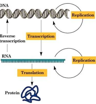
2.1.1 The Central Dogma
DNA (deoxyribonucleic acid) is widely described as the building block of life. It is a double helical structure consisting of a sequence of four nucleotide bases: Adenine (A), Guamine (G), Thymine (T), and Cystosine (C). So, the DNA sequence looks something like ‘ACTGGCTTACGGA’.
Figure 2.1: The central dogma of molecular biology. (Source: Dr. John S. Choinski)
2.1.2 Microarrays
Microarrays (Figure 2.2) are chips that are used to detect the RNA levels of genes. A single microarray chip is capable of simultaneously measuring the expression levels of sev-eral thousand genes. This simultaneous measurement goes a long way in our understanding of gene regulation and gene to gene interaction [PYK+
03, CMRR09]. However, microarray data is also characterized by a high level of ’noise’ and not all measurements can always be used. There are also numerous normalization methods to process raw microarray data, and there is considerable debate on which methods are best.
Figure 2.2: Microarrays show expression levels of thousands of genes (Source: http://www.wormbook.org)
2.1.3 Gene Interaction network
We still don’t completely understand the functions of thousands of genes, or all the gene to gene interactions. The gene interaction network is still in the process of being mapped. It is generally agreed that there is considerable redundancy built-in, and that genes interact with each other to produce proteins in complex ways. For example, Figure 2.3 illustrates some of the ways in which genes may interact with each other. Many diseases are now being explained by the disruption of these gene to gene interactions.
2.1.4 Ontologies & Pathways
Gene Ontology (GO) is a collection of controlled vocabularies that describe the biology of a gene product [ABB+
Figure 2.3: Gene interaction networks. (Source: Lee et al. ‘Transcriptional regulatory networks in Saccharomyces cerevisiae. In Science , vol. 298, 2002)
in three independent ontologies: Biological Process, Cellular Component, and Molecular function, each represented by a directed acyclic graph (DAG). Gene Ontology has proven to be very important for secondary analysis of microarray expression data [LWY04], and a wide range of tools have been developed to aid in this analysis. A comprehensive anal-ysis of the available tools is given by Khatri [KD05]. Some of the prominent ones are ontoTools [DKB+
03], GOminer [ZFW+
03], and GOstat [BS04].
validation for the clusters. We use statistical significance tests to determine if the genes in a cluster belong to a specific Biological Process. A biologically meaningful cluster would consist of many genes that are annotated to a specificGO term.
Kyoto Encyclopedia of Genes and Genomes (KEGG) [KAG+
07] pathways are a manually curated collection of maps incorporating our knowledge on molecular interactions and networks. It is a systematic collection of biological processes and systems that integrates functional, chemical and molecular information. KEGG has disease specific maps (e.g., cancer), and reflects current knowledge of pathway deregulations that are crucial in the propagation of the disease. We use KEGG pathways as a ‘gold standard’ against which we validate our experimental results.
Chapter 3
Clustering
Clustering is a popular data exploration technique widely used in microarray data analysis. Clustering methods provide a useful technique for exploratory analysis of microar-ray data since they group genes with similar expression patterns together. It is believed that genes that display similar expression patterns are often involved in similar functions. Various clustering techniques have been proposed [JTZ04, HKK05]. Some of the popular techniques for clustering genes employ k-means [THC+
99], hierarchical clustering [ESBB98], self-organizing maps [TSM+
finished chapter here.
We have developed a new algorithm, SigCalc, that is able to develop biologically meaningful gene clusters. Our algorithm uses elements of subspace projection, along with existing knowledge on gene associations to come up with multiple new cluster sets. Each of these new cluster sets reveal biological associations that were not apparent from clustering the original gene expression data. Our algorithm is fundamentally different from the con-ventional subspace clustering methods in that it projects the original expression data into a different information space where genes are described in relative terms against a chosen subset of genes called landmarks.
3.1
Related Clustering Algorithms
3.1.1 Subspace Clustering
3.1.2 Semi-supervised Clustering
Semi-supervised clustering [BBM04a, BBM04b, WCRS01] uses existing domain knowledge to guide the clustering process. One popular method is constraint based cluster-ing, where pairwise constraints (i.e ‘must-link’ and ‘cannot-link’ pairs) guide the clustering. The objective function of the underlying clustering algorithm is modified to accommodate these constraints. Our method differs from this clustering method as it does not constrain all the landmark genes to belong to one cluster. In our biological context, it is not unusual for genes to have more than one function.
3.1.3 Random Projection
3.2
Methods
3.2.1 Microarray Datasets
We use three yeast Saccharomyces cerevisiae datasets in our experiments. First, we use the cell cycle dataset of Spellman [SSZ+
98] available in R [R D06], comprising of 5,624 genes and 77 samples. Second, we use the diauxic shift dataset of DeRisi [DIB97] com-prising of 6,066 genes and 7 samples, and third the heat shock dataset of Gasch [GSK+
00] comprising of 6,097 genes and 14 samples. We applied a filter based on variation in gene expression, to focus our computations on informative genes across the samples. We selected genes that had a standard deviation greater than 0.35, and selected only those genes that were annotated in the biological process ontology of GO. The reduced datasets had 2288 genes for Spellman, 2,794 genes for DeRisi and 4,508 genes for Gasch. We then normalized them to a mean of zero and a standard deviation of one.
3.2.2 SigCalc Algorithm
We formally define the signature calculation algorithm, SigCalc, in this subsec-tion. Let M represent the microarray table consisting of n genes and m samples. SigCalc takes as input a microarray table M and a biological process. Using Gene Ontology, we find all the GO terms associated with the chosen biological process, and then find all genes associated with these GO terms.
Figure 3.1: SigCalc algorithm. -1.172 0.199 0.725 0.313 0.725 YAL009W -2.170 0.129 0.890 0.858 -0.521 YAL008W 0.440 0.864 -0.501 0.134 -0.783 YAL007C 0.670 0.110 1.203 2.036 0.069 YAL005C -2.214 1.089 0.947 -0.886 0.789 YAL004W 0.639 -0.658 -0.658 0.869 0.080 YAL003W 0.933 -0.671 1.783 1.375 -0.001 YAL002W S5 S4 S3 S2 S1
(a) Microarray expression data matrix. The se-lected landmark genes are highlighted.
0 0.075 0.507 YAL009W 0.090 0.187 0.380 YAL008W 0.798 0.658 0.681 YAL007C 0.470 0.683 0.093 YAL005C 0.075 0.0 0.683 YAL004W 0.741 0.918 0.347 YAL003W 0.507 0.684 0.0 YAL002W YAL009W YAL004W YAL002W
(b) Gene signature matrix, where each row represents a gene signature.
Figure 3.2: Conversion of gene expression data to gene signatures using SigCalc
etc. The algorithm for calculating the gene signatures, given a biological process, is shown in Figure 3.1. TheSigCalcalgorithm would convert a microarray data matrix (Figure 3.2(a)) into a gene signature matrix (Figure 3.2(b)).
subspace. If two genes are close to each other in this projected subspace, then these two genes may show similar expression patterns relative to the landmark genes. By varying the set of landmark genes, we are able to vary this subspace.
The SigCalc algorithm uses a distance function, dist, to measure the similarity between two gene vectors in microarrayM. A variety of distance metrics such as Euclidean and cosine distances, or some other variants can be used. In our experiments we used the pearson correlation, a popular similarity metric [D’H05] to arrive at the distance. Given two gene vectors −→gi and−→gj, the pearson correlation is given by:
cor(−→gi,−→gj) =
covariance(−→gi,−→gj) p
covariance(−→gi,−→gi)×covariance(−→gj,−→gj)
To calculate our gene signatures, we define our correlation distance function as:
dist= 0.5×(1−cor(−→gi,−→gj))
3.2.3 Clustering algorithms used
We chose two popular algorithms, tight clustering that is based on k-means clus-tering and self organizing maps (SOM) [TSM+
99] to validate our Gene Signature model. The Tight Clustering algorithm [TW05] is a re-sampling based algorithm, that uses k-means clustering, to return genes that are clustered together consistently upon resampling. Re-sampling based methods have been found to return consistent clusters [YMB03, ACPS06]. The Tight Clustering algorithm forms clusters that are stable and tight, and excludes genes from clusters that are ‘noisy’ and only serve to dilute the cluster. It has been widely used in microarray data clustering [ZKH+
05, HWP06, KMPG06, CSBW06]. SOM is another clustering algorithm we used in our experiments. We use the R [R D06] implementation of SOM.
3.2.4 Cluster validation
3.2.5 Significant GO terms from clustering microarray data
Clustering of Microarray data
(a) Significant GO terms in microarray data
Clustering on Microarray data
Gene Signature G
clustering with landmark genes linked to 'electron transport' Gene Signatureignature
clustering with landmark genes linked to ' proteolysis'
(b) Significant GO terms in microarray data and gene signatures
Figure 3.3: Significant GO terms found using clustering on microarray data vs. clustering on gene signatures.
We partition the microarray data M (n genes × m samples) into N clusters (N = 100 for results presented). We evaluate the biological significance of each cluster as follows: For a set of genes in a cluster, we evaluate if there are any GO terms that are over-represented than would be expected by chance. We evaluate the probability of a set of genes in a cluster being associated with the same GO term by using the hypergeometric distribution of the genes in the cluster. The probability of a cluster of size S containing x genes belonging to a particular GO term, given that the reference dataset ofN genes has a total of Agenes belonging to that particular GO term is:
P r{X=x|N, A, S}=
A x
N −A S−x
N S
associated with a particular GO term [DKM+
03]. A cluster is considered to contain a significant GO term only if it has more than two genes associated with a specific GO term, and has a p-value less than 0.01. We used theGOstat package [BS04] for the hypergeometric test to find the set of statistically significant GO terms.
The set of significant GO terms for the original microarray clusters is the union of the significant GO terms for all of the clusters. This set of GO terms will be called the Original GO terms, as shown in Figure 3.3(a).
3.2.6 Significant GO terms for a dataset using gene signatures
We build the gene signature matrix, for a selected biological process, by using SigCalc as given in Figure 3.1. Next, we partition the n ×kgene signature matrix into N clusters (N = 100, i.e., the same number of clusters that were used for clustering the original microarray data). All other parameters for the clustering algorithm were kept the same as were used to cluster the original microarray data, as described in the previous section. This clustering of Gene signatures will be termed as Gene Signature Clustering. The set of significant GO terms from the clusters is derived using the hypergeometric distribution in the same way as described in the previous section. This set of significant GO terms obtained by clustering gene signatures, associated with a set of landmark genes, will be calledlandmark GO terms, as shown in Figure 3.3(b).
calledunique GO terms.
3.2.7 Unique GO terms common across datasets
3.3
Results and Discussion
3.3.1 Results
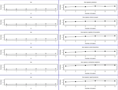
In the gene signature model, genes are points in a projected subspace whose co-ordinates are the landmark genes. The gene signature consists of relative distance to these landmark genes. So, by changing the landmark genes, a different perspective of the sub-space can be obtained. Even using the same clustering algorithm, we can get different sets of clusters by changing this subspace. We repeated gene signature clustering for several biological processes (i.e., we used several different sets of landmark genes). The details for theoverlapping GO terms and theunique GO terms, using different biological processes as landmarks for the Spellman dataset are shown in Table 3.1.
Table 3.1: Details of overlaps between significant GO terms found by original clustering of microarray data, and those found by using gene signature clustering for the Spellman dataset.
Biological process used Number of Number of Number of Number of for landmark genes Landmark Original Overlapping Unique
Genes GO terms GO terms GO terms
proteolysis 51 182 120 41
electron transport 20 182 126 44
regulation of transcription 100 182 126 41
protein biosynthesis 194 182 101 20
carbohydrate metabolism 121 182 142 58
signal transduction 52 182 121 53
ubiquitin-dependent protein 40 182 129 61
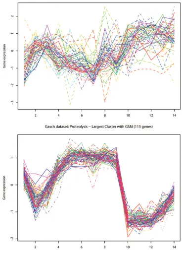
used, but did not cluster together when the original microarray data was used. Some of these genes are shown in Figure 3.4.
2 4 6 8 10 12 14
−2 −1 0 1 2 Microarray data Samples Expression Value
0 5 10 15 20 25
0.2 0.4 0.6 0.8 Gene Signatures Signature Value YER075C YGR279C YJL157C YLL021W YLR229C YLR452C YNL188W YOR061W
(a) Comparison of microarray expression data with gene signatures for genes that clustered together using gene signatures. Gasch dataset: Genes associated with
multi-organism process (GO:0051704) were
clus-tered together.
2 4 6 8 10 12 14
−2 −1 0 1 2 Microarray data Samples Expression Value
2 4 6 8 10
0.2
0.4
0.6
0.8
Gene Signatures
Signature Value YGL170C
YGR221C YJL157C YLL021W YNL145W YOR242C
(b) Comparison of microarray expression data with gene signatures for genes that clus-tered together using gene signatures. Gasch dataset: Genes associated withreproduction
(GO:0000003) were clustered together.
Figure 3.4: Comparison of expression values vs gene signatures for genes known to belong to be annotated to the same GO term.
Number of clusters
Number of GO terms
50 100 150 200 250 300
20 40 60 80 100 120 140
carbohydrate metabolism electron transport
20 40 60 80 100 120 140 protein biosynthesis proteolysis regulation of transcription
50 100 150 200 250 300 signal transduction
50 100 150 200 250 300
ubiquitin−dependent protein
Total GO terms
Common GO terms Unique GO terms
Figure 3.5: Number of GO terms for varying number of clusters. For each landmark, a number of unique GO terms are found irrespective of the number of clusters.
GO term discovered is not immediately clear in this case, there might be some inherent relationships between them that are worth further investigation. Nonetheless, there were many other GO terms discovered using signatures (but not with the original expression data) whose associations with signature terms are much clearer. Some of these terms are investigated in detail in the discussion section.
clusters from 20 to 140. The results are shown in Figure 3.5. These indicate that there are a substantial number of unique GO terms for each set of landmark genes, that are largely independent of the number of clusters.
Table 3.2: CommonUnique GO Terms between datasets (taken two at a time), using Tight Clustering algorithm. Spellman-Gasch (2038 genes) Gasch-DeRisi (2474 genes) Spellman-DeRisi (1408 genes)
Biological process Unique GO terms Unique GO terms Unique GO terms
used to get Spell- Gasch Common Gasch DeRisi Common Spell- DeRisi Common landmark genes -man (p-value) (p-value) -man (p-value)
proteolysis 28 89 12 (7.7x10⁻⁶) 117 80 27 (1.2x10⁻⁷) 32 17 3 (3.4x10⁻²)
electron transport 28 89 9 (1.3x10⁻³) 121 125 28 (6.5x10⁻⁴) 47 59 15 (1.6x10⁻⁶)
regulation of trans. 23 57 5 (1.3x10⁻²
) 83 76 20 (1.6x10⁻⁶
) 31 24 5 (2.8x10⁻³
) protein biosynthesis 32 85 7 (2.6x10⁻²
) 101 83 20 (1.4x10⁻⁴
) 21 53 1 (3.2x10⁻¹
) carbohydrate meta. 22 72 7 (1.4x10⁻²
) 97 81 16 (3.6x10⁻³
) 28 33 1 (3.6x10⁻¹
) signal transduction 43 68 23 (1.0x10⁻¹⁵
) 76 98 22 (1.6x10⁻⁶
) 44 28 8 (1.6x10⁻⁴
) protein folding 29 72 10 (6.3x10⁻⁵
) 110 81 31 (4.9x10⁻¹¹
) 24 32 4 (1.8x10⁻²
) intracellular protein 38 79 9 (5.1x10⁻³
) 137 83 25 (7.6x10⁻⁵
) 33 43 7 (2.4x10⁻³
) lipid metabolism 43 73 17 (1.3x10⁻⁸
) 97 85 27 (6.4x10⁻⁹
) 32 27 4 (2.6x10⁻²
) ribosome biogenesis 66 94 22 (4.4x10⁻⁷
) 111 124 22 (1.2x10⁻²
) 55 30 9 (2.4x10⁻⁴
Table 3.3: CommonUnique GO Terms between datasets (taken two at a time), using SOM algorithm.
Spellman-Gasch (2038 genes) Gasch-DeRisi (2474 genes) Spellman-DeRisi (1408 genes)
Biological process Unique GO terms Unique GO terms Unique GO terms
used to get Spell- Gasch Common Gasch DeRisi Common Spell- DeRisi Common landmark genes -man (p-value) (p-value) -man (p-value)
proteolysis 28 90 1 (1.3x10⁻¹) 90 56 17 (4.4x10⁻⁶) 29 49 8 (4.6x10⁻⁴)
electron transport 55 76 23 (1.1x10⁻¹¹) 97 52 17 (4.13x10⁻⁶) 36 57 3 (2.4x10⁻¹)
regulation of trans. 39 79 15 (5.0x10⁻⁷
) 69 45 8 (9.8x10⁻³
) 32 40 1 (2.9x10⁻¹
) protein biosynthesis 64 71 19 (2.07x10⁻⁷
) 77 69 10 (2.8x10⁻²
) 20 72 2 (2.9x10⁻¹
) carbohydrate meta. 37 73 11 (1.3x10⁻⁴
) 76 60 13 (4.2x10⁻⁴
) 42 45 2 (2.5x10⁻¹
) signal transduction 74 74 14 (2.5x10⁻³
) 92 61 10 (3.7x10⁻²
) 45 36 6 (1.9x10⁻²
) protein folding 47 71 5 (1.7x10⁻¹
) 77 44 5 (1.4x10⁻¹
) 39 36 4 (9.6x10⁻²
) intracellular protein 41 98 16 (3.5x10⁻⁶
) 113 51 18 (6.0x10⁻⁶
) 42 46 6 (1.4x10⁻²
) lipid metabolism 47 83 9 (2.3x10⁻²
) 84 64 12 (5.5x10⁻³
) 73 37 0 (1.3x10⁻²
) ribosome biogenesis 40 71 19 (1.6x10⁻¹¹
) 99 77 9 (1.4x10⁻¹
) 27 55 0 (9.7x10⁻²
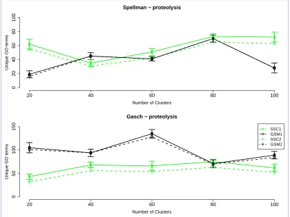
We also compared our gene signature model against a base line approach built using a k-nn classifier. We used ten fold cross validation to impute functional annotations using k-nn and clusters obtained from our model. For all the landmarks tested, our approach produced a higher classification accuracy than the k-nn based approach, irrespective of ’k’, as shown in Figure 3.6
Finally, in order to validate the effectiveness of our approach, we compared our model, using tight clustering with gene signatures (GSM), to an existing semi-supervised clustering (SSC) model. For the SSC, the landmark genes were considered as ’must-link’ constraints. All the landmark genes were thus clustered together in one cluster using the SSC. We then compared our model to the SSC by comparing the number of unique GO terms found for each set of landmark genes.
SSC1 denotes the number of unique GO terms found by using landmark genes as constraints in SSC.GSM1 denotes the number of unique GO terms found by using the gene signature model. SSC2 denotes the number of unique GO terms found for SSC if we remove the largest cluster (containing all the landmark genes) from analysis. GSM2 denotes the number of unique GO terms found using the gene signature model if we remove the largest cluster from analysis.
2 4 6 8 10 12 0 20 40 K Accuracy knn
20 40 60 80 100 120
0
20
40
Number of clusters
Accuracy
Gene signature: proteolysis
2 4 6 8 10 12
0 20 40 K Accuracy knn
20 40 60 80 100 120
0
20
40
Number of clusters
Accuracy
Gene signature: electron transport
2 4 6 8 10 12
0 20 40 K Accuracy knn
20 40 60 80 100 120
0
20
40
Number of clusters
Accuracy
Gene signature: regulation of transcription
2 4 6 8 10 12
0 20 40 K Accuracy knn
20 40 60 80 100 120
0
20
40
Number of clusters
Accuracy
Gene signature: protein biosynthesis
2 4 6 8 10 12
0 20 40 K Accuracy knn
20 40 60 80 100 120
0
20
40
Number of clusters
Accuracy
Gene signature: carbohydrate metabolism
2 4 6 8 10 12
0 20 40 K Accuracy knn
20 40 60 80 100 120
0
20
40
Number of clusters
Accuracy
Gene signature: signal transduction
x
x
x
x x
20 40 60 80 100
0 20 40 60 80 100
Spellman − proteolysis
Number of Clusters
Unique GO terms
o o o o o x x x x x o o o o o x
x x x x
20 40 60 80 100
0
50
100
150
Gasch − proteolysis
Number of Clusters
Unique GO terms
o o o o o x
x x x x
o o o o o x o x o SSC1 GSM1 SSC2 GSM2
in one dataset than in the other. One difference between the two models is that the SSC forces the landmark genes in one cluster. This could lead to a large, less compact cluster, especially in cases where there are a large number of landmark genes with varied expression patterns. For example, for the Spellman dataset (Figure 3.8), the gene expression pattern of the landmark genes correlates well and the SSC model performs better, whereas for the Gasch dataset (Figure 3.8) the gene expression pattern of the landmark genes does not correlate well, and the GSM performs better.
3.3.2 Discussion
These results indicate that clusters using gene signatures have biological signif-icance, and that many of these gene associations are not found using clustering on the original microarray expression datasets. Each set of landmark genes carries the potential of defining its own set of clusters from the same dataset.
To study this more closely, we examined several pairs of biological processes, i.e., the biological process that was used for selecting the landmark genes and its corresponding common unique GO terms found across datasets. For the Spellman and Gasch datasets, we analyze two of these biological processes (proteolysis and electron transport) and some of their commonunique GO terms. These are listed in Table 4.
Proteolysis and Transcription: The connection between proteolysis and transcrip-tion has been well established. Proteolysis has been known to regulate transcriptranscrip-tion [MCR+
86, WSB+
Proteolysis and Phosphorylation: The two processes interweave and interact with each other resulting in chromosome replication and segregation in budding yeast [Des97]. The two processes have also been linked to the Cdc28 protein kinase complex and other proteins involved in the budding yeast [TTNF92]. Recently it was reported that the hu-man homolog of Mcm10 (a protein in yeast involved in DNA replication) is also regu-lated by proteolysis and phosphorylation during the cell cycle [IYH01]. One article ex-plores how the signaling molecule Hedgehog prevents the proteolyis (by phosphorylation) of Cubitus interruptus (Ci-155) transcriptional activator [PK02] and another touches on how phosphorylation-induced proteolysis eliminates unwanted by-products of protein ki-nases [EQC05].
Electron Transport and Oxidative Phosphorylation: The relationship between these two processes has been studied across organisms. The inhibitory effects of Salicylic Acid on both the mitochondrial functions were presented in [XC99]. Salicylic acid inhibited mitochondrial electron transport which in turn inhibits oxidative phosphorylation. A recent article has studied the neurological diseases in humans and found that they may be caused by a defective electron transport system and its effect on oxidative phosphorylation [Nus05]. Many other papers have also studied the relationship between these processes[MS66, WO70, VVS78, Hat85].
Electron Transport and ATP Synthesis: The relationship between these two pro-cesses has also been well studied. Allakhverdiev [ANT+
pro-cesses on the frequencies and harmonics of yeast Saccharomyces cerevisiae were studied in [MNV+
05]. Faxen [FGAB05] and Belevich [BVW06] study the mechanics of the inter-mediate steps between Electron transport and energy requiring processes like ATP synthesis. We chose the Biological Process Ontology to select the landmark genes. Neverthe-less, other sources that list genes belonging to a particular process or function can also be used. The biologist should also be able to define their own set of landmark genes and use these as the co-ordinates for projection.
We showed that clustering on gene signatures using different sets of landmark genes creates new sets of clusters that are different from the clusters obtained from the original microarray data. Genes in these new clusters reveal biological insights that were not present in the clustering of the original microarray data. We also showed that the new clusters are associated with biological terms that have some ties with the genes used for landmark selection.
3.4
SigClust application package
pro-vide internal validation measures, whereas our package validates the biological significance of the new clusters by retrieving significant ontology and pathway terms associated with the new clusters.
Essentially, our technique is a two step process. In the first step, we use our SigCalc algorithm to project the microarray data onto landmark genes. The output of this step is a set of gene signatures. In the second step, we use existing clustering algorithms to cluster gene signatures derived in the first step. We then validate the new clusters by evaluating significant GO/KEGG/PFAM terms associated with genes in the new clusters.
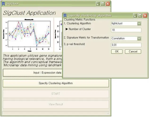
The SigClust application is able to process probe level data of two organisms, yeast and homo sapiens. This is to be extended to rat and zebrafish. The application interface is shown in Figure 3.9
3.4.1 Clustering Algorithms
We have selected four popular clustering algorithms. These are:
1. Tight clustering - This is a re-sampling based algorithm [TW05], that uses k-means clustering, to return genes that are clustered together consistently upon resampling. Re-sampling based methods have been found to return consistent clusters [YMB03, ACPS06]. The Tight Clustering algorithm forms clusters that are stable and tight, and excludes genes from clusters that are ‘noisy’ and only serve to dilute the cluster. It has been widely used in microarray data clustering [ZKH+
05, HWP06, KMPG06, CSBW06].
pression data. Essentially, the data points are arranged in a hierarchy of nested subsets. There are numerous variations in the similarity measures (e.g., single-link, complete-link etc.) In our application we use two clustering algorithms implemented in the cluster package in R [R D06], i.e., Clustering Large Applications (CLARA), and Divisive Analysis Clustering (DIANA).
3. Self Organizing Maps - These are based on neural networks [Koh00] and are also a popular algorithm for clustering of gene expression data [RWN03]. These are par-ticularly useful for high dimensional data, and when classifying noisy or incomplete data [CWRT03]. In our application, we use thesom package R [R D06] implementa-tion of SOM.
3.4.2 Cluster validation
We use external validation criteria to test for the ’goodness’ of the clusters. We use Gene Ontology (GO) [ABB+
00], Kyoto Encyclopedia of Genes and Genomes (KEGG) [KAG+08], and Protein Family (PFAM) database [FTM+08a] to validate the biological
Chapter 4
Classification
The use of DNA microarrays has resulted in the identification and monitoring of numerous cancer marker genes. These genes have been widely used to differentiate not only cancerous tissue samples from normal healthy ones, but also between different sub-types of cancer [GST+
99, SFR+
02, LLH+
04, Gho06, RHS+
08]. From a diagnostic point of view, it is important to correctly identify cancerous tissue so that the most appropriate treatment can be given as early as possible.
Numerous classifiers have been proposed and evaluated on their comparative accu-racy in correctly identifying cancer tumors [DFS02, DB03, GdNW04, TNX+
05, HKDSB08, HD08, LX09]. The most prominent of these classifiers are Prediction Analysis of Microarray (PAM) [THNC02], Support Vector Machines (SVM) [Vap95, GWBV02],k-nearest neighbor (k-NN) [Rip96], C4.5 decision trees (DT) [Qui93], Top Scoring Pair (TSP) [GdNW04], and k-Top Scoring Pair (k-TSP) [TNX+05]. Methods like bagging and boosting [DZ04] have also
Table 4.1: Microarray datasets used for classification
Dataset Platform Genes (N) Samples (M) Reference
Colon cDNA 2000 62 Alon [ABN+
99]
Leukemia Affy 7129 72 Golub [GST+
99]
CNS Affy 7129 34 Pomeroy [PTG+
02]
DLBCL Affy 7129 77 Shipp [SRT+
02]
Lung Affy 12533 181 Gordon [GJH+02]
Prostate1 Affy 12600 102 Singh [SFR+
02]
Prostate2 Affy 12625 88 Stuart [SWB+
04]
Prostate3 Affy 12626 33 Welsh [WSS+01]
GCM Affy 16063 280 Ramaswamy [RTR+
01]
Results from these studies indicate that there is no single classifier that has the highest accuracy for all the microarray expression datasets.
We introduce a novel method to combine gene expression data from pairs of genes to improve the accuracy of the PAM [THNC02] classifier for binary classification. PAM is one of the most widely employed statistical methods for classifying microarray expression data. Its accuracy over most datasets is extremely good. However, for some datasets other classification methods like SVM and TSP far outperform PAM [TNX+05]. We propose a
novel method that would improve the performance of PAM significantly for these datasets while retaining the high accuracy of PAM over the other datasets. The proposed method uses the expression values derived from gene pair combinations, instead of the original expression values of genes, as the input for PAM.
4.1
Gene Doublets
Let there be N genes {g1, . . . , gN} in a tissue sample, and let there be M such
tissue samples {x1, . . . , xM}. The cancer dataset could then be represented as matrix Q
of dimension N×M. Then, gij would denote the expression value of the i-th gene, i ∈
{1, . . . ,N} in the j-th sample, j ∈ {1, . . . ,M}. The gene vector gi = {gi1, . . . , giM} would
denote the expression value of the i-th gene across the M tissue samples, and the column vector xj = {g1j, . . . , gN j} would represent the j-th tissue sample across the N genes.
The class labels for the tissue samples are represented by vector y = {y1, . . . , yM}, where
yj ∈ {C1, . . . , CK}, the set of all class labels. For our binary classification problem, K= 2,
whereC1 denotes cancerous andC2 denotes normal tissue samples.
For each pair of genes i,p ∈ {1, . . . ,N},1 ≤i < p ≤ N in a dataset, we define a positive doublet vector and a negative doublet vector as
gigp+ ={gi1+gp1, gi2+gp2, . . . , giM+gpM} (4.1)
gigp− ={gi1−gp1, gi2−gp2, . . . , giM−gpM} (4.2)
Input: Gene Expression MatrixQwithN genes andM samples, class vector y for theM samples and T the number of the genes required for analysis.
Output: Unique doublets
1. Compute t-scores for matrix Qusing class vectory.
2. Make an ordered list Θ of all the genes gi, in decreasing value of their absolute t-score.
3. Take the top T genes from the ordered list Θ, and extract their expression values fromQ. The new expression matrix Q′ hasT rows and M columns.
4. Make doublets fromQ′ to get a new matrix Q′′, with T(T−1) rows and M columns. For details refer Section 4.1
5. Compute t-scores for matrix Q′′ using class vectory.
6. Make an ordered list Ω of all the doublets gigp inQ′′, in decreasing value of their absolute t-score.
7. Initialize φas an empty list.
8. forall doublets gigp in Ωdo(in decreasing absolute t-score order); If neither of the genes in the doubletgigp is inφ, then add doublet
gigp toφ
9. Return φ
Algorithm 1: Obtaining unique doublets from microarray gene expres-sion data.
4.2
Microarray Data and Classification Methods
The microarray data is taken from several studies, as shown in Table 4.1. These are the same datasets that were used in [TNX+
05] for their comparison of various classifiers and were obtained from their website (http://www.bme.jhu.edu/%7Eactan/KTSP/). The microarrays consist of expression data for tissues associated with colon, blood, lung, breast, prostate, and cancer of the central nervous system. The number of samples and the number of genes in each study is also shown in Table 4.1. The datasets were processed to have a minimum value of 10, then log2 transformed and all samples standardized to zero mean and
4.2.1 Classifier Performance
We evaluate the performance for the prediction analysis of microarrays (PAM) clas-sifier, using doublets as input data. PAM is a statistical method widely used for classifying both binary and multi-class microarray data. It is based on the nearest shrunken centroid principle. We use the R [R D06] implementation of PAM [THNC02] (version 2.3.0) for all our experiments. Similar to [TNX+
05], for each dataset we do a ten-fold cross-validation on the training set to determine the subset of genes that are most informative for the clas-sification model. This process makes PAM model non-deterministic; i.e., depending on how the training set is folded into ten subsets, the set of genes identified may differ. Nonethe-less, this approach is widely used in practice as it makes the model more robust. In our experiments, we run the tests ten times and report the accuracy from ten runs.
4.2.2 Classification Accuracy
We use the LOOCV (Leave One Out Cross Validation) method to estimate the classifier accuracy. For each samplexjin the dataset, we use the rest of theM−1 samples in
the dataset to predict the class of thexjsample. The classification accuracy for each dataset
is the ratio of the number of correctly classified samples (True Positives+True Negatives) to the total number of samples (M) in that dataset.
Figure 4.1: Accuracy ofD-PAM for topn% genes compared to the PAM accuracy for each of the nine datasets.
For the accuracy of the datasets using doublets, we first compute the t−scores for the genes and arrange them in decreasing absolute value of this score. The formula used to calculate this score is
t−score= X¯C1 −X¯C2
r σ2
C1
NC1 +
σ2 C2
NC2
(4.3)
where ¯XC1,X¯C2 represent the class means;σ
2 C1, σ
2
C2 represent the variances; andNC1, NC2 represent the number of samples for the two classesC1 andC2, respectively.
Table 4.2: LOOCV accuracy of classifiers for binary class expression datasets
Method Leukemia CNS DLBCL Colon Pros.1 Pros.2 Pros.3 Lung GCM Avg.
TSP∗ 93.80 77.90 98.10 91.10 95.10 67.60 97.00 98.30 75.40 88.26
k-TSP∗ 95.83 97.10 97.40 90.30 91.18 75.00 97.00 98.90 85.40 92.01 DT∗ 73.61 67.65 80.52 80.65 87.25 64.77 84.85 96.13 77.86 79.25 NB∗ 100.00 82.35 80.52 58.06 62.75 73.86 90.91 97.79 84.29 81.17
k-NN∗ 84.72 76.47 84.42 74.19 76.47 69.32 87.88 98.34 82.86 81.63 SVM∗ 98.61 82.35 97.40 82.26 91.18 76.14 100.00 99.45 93.21 91.18
PAM 94.03 82.35 85.45 89.52 90.89 81.25 94.24 97.90 82.32 88.66 D-PAM† 97.22 95.59 94.81 90.16 91.57 85.79 96.67 100.00 84.50 92.92
†Results from taking the top 1% of genes for making unique doublets.
4.3
Results
Figure 4.1 compares the accuracy of the standard PAM classifier to that of D-PAM obtained by taking the topn% genes, for the nine datasets. It can be seen that even taking a small percentage of the top genes and making doublets substantially improves the performance of PAM. Table 4.2 shows the comparative accuracies of the various classifiers for different datasets. The D-PAM classifier outperforms the standard PAM classifier for almost all of the datasets. For the two of the datasets,CNS and DLBCL, this gain is substantial. For the CNS dataset the accuracy has increased from 82.35% to 95.59%, and for the DLBCL dataset the accuracy has increased from 85.45 % to 94.81%. By using doublets for PAM, the average accuracy of the classifier for the nine datasets has increased from 88.66% to 92.92%.
4.4
Discussion
The genes comprising the top doublets also provide easily interpretable results, as compared to other methods like SVM. Although SVM may provide a higher accuracy than PAM, it is essentially a black box and no insight can be gained regarding biomarker genes. Doublets on the other hand are easily interpretable. They identify which genes and which gene pairs can serve as biomarkers for tumor classification. Compared to PAM, D- PAM also provides another information layer to the analysis because the doublets also indicate if the relation between the two genes is positive (i.e. if the gene pair is a positive doublet) or negative (if it is a negative doublet).
Chapter 5
Ontology and Pathway Analysis
Cancer research has shown that cancer is caused by the simultaneous deregulation of many interacting cellular pathways. These pathways include oncogenes (i.e., cancer causing genes), tumor suppressor genes and DNA repair genes [KAG+
07]. Molecular biology and high throughput technologies are increasingly being used for the diagnosis, survival prediction, and treatment of cancer. However, there still remain many genes and pathways whose role in the cause and progression of cancer is not clearly understood. There is also a pressing need to understand the higher level functions and interactions that these genes contribute to. In this chapter, we present the results of a meta-analysis of cancer datasets, from an ontological and pathway perspective.
Over the last few years, there has been an explosion in the number of cancer microarray datasets available in public repositories. However, the number of research papers using multiple datasets in their analysis have been limited [SFKR04, RYS+04]. While
and KEGG pathways, there haven’t been many papers that have mapped multiple cancer datasets to GO or KEGG. Mapping and mining multiple microarray datasets may yield insights that were not possible by using just one, or at best, a few datasets.
The results presented in this section should be viewed with the knowledge that the fold changes linked to ’over-expression’ and ’under-expression’ are open to biological interpretation. The meta-analysis also suffers from the drawback that the datasets have been taken from diverse platforms and they contain diverse number of genes, and that the datasets themselves have been normalized separately. Nevertheless, we believe that the global cancer map presented here presents some salient pathways that are unique to specific cancers, and also some pathways that are common across cancer types. We have created global cancer maps for Gene Ontology (GO), Kyoto Encyclopedia of Genes and Genomes (KEGG) pathways and Protein Families database (PFAM).
5.1
Background
5.1.1 Gene Ontology
Gene Ontology (GO) is a collection of controlled vocabularies that describe the biology of a gene product [ABB+
00]. We have previously described the ontology structure and it’s utility in Chapter 2.
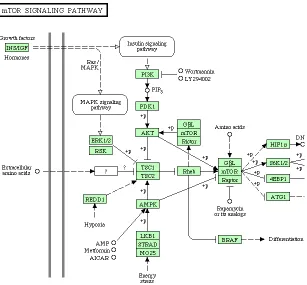
5.1.2 KEGG Cancer Pathways
Figure 5.1: The mTOR pathway that is closely linked with cancer. The rectangles represent genes/gene products and the circles represent metabolic compounds. (Source: http://www.genome.jp/kegg/pathway.html#disease)
current knowledge about that pathway. These pathways incorporate products of oncogenes (i.e., tumor causing genes), tumor suppressor genes, and dna repair genes [KAG+07].
5.1.3 PFAM database
The PFAM database is a collection of protein families [FTM+
08b]. A protein consists of several functional regions, and the different combinations of these functional regions give rise to diversity in protein structure and function. In our analysis, we will determine if a set of genes is related to a particular protein family in a statistically significant way.
5.2
Materials and Methods
5.2.1 Datasets
For the meta-analysis of human cancer microarray datasets, we took a total of 87 datasets, containing 5,126 cancer tissue samples, comprising of 25 different types of cancer, and several microarray platforms. The details of the datasets used are given in Table A.2. For the meta-analysis of mouse datasets, we took a total of 18 microarray datasets (Table A.2). All the microarray data, for both organisms, was downloaded from Gene Expression Omnibus (GEO) and Stanford Microarray Database (SMD). To the best of our knowledge this is the largest meta-analysis of microarray datasets to date. It is also the first analysis that compares the results obtained from the meta-analysis of two organisms.
5.2.2 Data pre-processing
and setting to 10 any value that was less than 10). For spotted cDNA datasets, we used the log2 ratio between the measured sample and the control sample. Any gene that had more
than 25% values missing was discarded from further analysis. A gene was considered to be over-expressed in a dataset if it showed greater than two-fold increase (i.e., a log2 value
greater than 1) in expression levels in more than 80% samples in that dataset. Similarly, a gene was considered to be under-expressed in a dataset if it showed greater than two-fold decrease (i.e., a log2 value less than−1) in expression levels in more than 80% tumor
samples in the dataset. We next calculate the hypergeometric probability of this set of over (under) expressed genes being associated with a particular GO/KEGG/PFAM term.
5.2.3 Significant GO/KEGG/PFAM terms
We evaluate the probability of ‘significant GO/KEGG/PFAM terms’ associated with a set of genes using the hypergeometric distribution function. The probability of a set of genes of size S containing x genes belonging to a particular GO/KEGG/PFAM term, given that the reference dataset of N genes has a total ofA genes belonging to that particular GO/KEGG/PFAM term is:
P r{X=x|N, A, S}=
A x
N −A S−x
N S
whereXis a random variable representing the number of genes in a cluster, that are associated with a particular GO/KEGG/PFAM term [DKM+
specific GO/KEGG/PFAM term, and has a p-value less than 0.01. We used the GOstat package [BS04] for the hypergeometric test to find the set of statistically significant GO terms.
5.3
Results
For each dataset, we shortlisted the ‘over’ and ‘under’ expressed genes. Then we conducted two sets of analysis. In the first analysis, we determined the significant ontology and pathway terms separately for over-expressed and under-expressed genes. In the second analysis, we treated the set of ‘over’ and ‘under’ expressed genes as one set, and found significant pathway and ontology terms for this combined set.
5.3.1 Evaluating over and under expressed genes separately for significant pathway terms
The significant GO terms, found by the meta-analysis for all types of human cancer, is shown in Figure 5.2. The global map clearly shows GO terms that are closely associated with ‘over’ expressed genes, and GO terms that are closely associated with ‘under’ expressed genes. This meta-analysis shows the hotspots that exist in the cancer datasets. These hotspots are most clearly discernible for breast, leukemia and liver cancers.
To determine if some types of cancer are associated with particular GO terms, we conducted a similar analysis using only human breast cancer datasets. The results are shown in Figure 5.3.
Table 5.1: Known cancer pathways found by meta-analysis of human microarray datasets Cancer Types Number of Number of Number of known
Datasets tissue samples pathways found
All types 87 5,126 11
Breast 23 1,933 12
Leukemia 8 447 14
Kidney 5 267 9
Liver 6 498 13
Prostate 6 213 13
the Gene Ontology tree (Figure 5.4). This indicates that many over-expressed and under-expressed genes are mapped to separate parts of the Gene Ontology tree, and may be associated with different pathways.
5.3.2 Evaluating over and under expressed genes together for significant pathway terms
In our second analysis, we treated the ‘over-expressed’ and ‘under-expressed’ genes as one set. We then determined the significant pathway and ontology terms associated with this gene set, as previously described. Combining the two sets of genes is also biologically consistent because many pathways are deregulated by a combination of over-expressed and under-expressed genes.
from different microarray platforms, which may otherwise not be directly comparable. From the rank ordered list of significant GO, KEGG, and PFAM terms, we analyzed the top 50, 100, and 150 significant terms. The results from the top 150 ranked significant terms are presented here.1
To validate our result, we compared the ranked top 150 list, obtained from datasets of all cancer types, to the list of fifteen pathways already known to be closely associated with cancer. We also determined the ranked top 150 terms from all the breast, leukemia, kidney, liver, and prostate cancer datasets, and compared these ranked lists with the ‘gold’ standard KEGG pathways. In all the cases, a significant proportion of the fifteen pathways were discovered by our method. The results are shown in Table 5.1. The complete ranked list of the significant GO/KEGG/PFAM terms, for various cancer types, are given in the Appendix (Tables A.4 to A.21).
To further corroborate our ranked list, we text mined PubMed for any articles that had both the ontology term/pathway and ‘cancer’. Text mining is increasingly being used in life sciences research to keep abreast of current knowledge on a gene or protein. It is being used not only to keep the biological databases up to date [BCF+
07] but also to plan experiments and validate their results [KVH08]. The concept of using co-occurrence to indicate association has been
Table 5.2: Top five ranked significant GO terms using datasets from all cancer types.
GOID GO Term Abstracts
(‘cancer’)
GO:0006412 Translation 10,000
GO:0002009 Morphogenesis of an epithelium 1,072 GO:0009260 Ribonucleotide biosynthetic process 827 GO:0000087 M phase of mitotic cell cycle 593 GO:0055085 Transmembrane transport 865
Table 5.3: Top five ranked significant KEGG terms using datasets from all cancers
KEGG ID KEGG Path Abstracts
(‘cancer’) 00400 Phenylalanine, tyrosine and tryptophan biosynthesis 3,201 00290 Valine, leucine and isoleucine biosynthesis 790
04630 Jak-STAT signaling pathway 328
00720 Reductive carboxylate cycle (CO2 fixation) 29 00040 Pentose and glucuronate interconversions 642
Table 5.4: Top five ranked significant PFAM terms using datasets from all cancer datasets.
PFAM ID Protein Family Abstracts
(‘cancer’)
PF00047 Immunoglobulin domain 2,834
PF00191 Annexin 2,928
PF00131 Metallothionein 1,379
PF07654 Immunoglobulin C1-set domain 239
PF00061 Lipocalin / cytosolic fatty-acid binding protein family 242
used extensively in medical literature [YHF+
02, CHDS05].
Table 5.5: Top five ranked significant GO terms using datasets from breast cancer.
GO ID GO Term abstracts abstracts
(‘cancer’) (‘breast cancer’)
GO:0007599 Hemostasis 6,583 315
GO:0009611 Response to wounding 5,632 515
GO:0065008 Regulation of biological quality 3,369 525
GO:0051325 Interphase 10,000 1,395
GO:0000398 Nuclear mRNA splicing, via spliceosome 680 75
Table 5.6: Top five significant KEGG terms using datasets from breast cancer
KEGG ID KEGG Path Abstracts Abstracts
(‘cancer’) (‘breast cancer’)
00230 Purine metabolism 10,000 1,157
00010 Glycolysis / Gluconeogenesis 2,464 149
00360 Phenylalanine metabolism 4,090 194
00220 Urea cycle and metabolism of amino groups 900 51
00510 N-Glycan biosynthesis 145 9
Table 5.7: Top five ranked significant PFAM terms using datasets from breast cancer.
PFAM ID Protein Family Abstracts Abstracts
(‘cancer’) (‘breast cancer’)
PF00227 Proteasome A-type and B-type 131 8
PF01454 MAGE family 175 22
PF07654 Immunoglobulin C1-set domain 239 42
PF00055 Laminin N-terminal (Domain VI) 53 4
PF00458 WHEP-TRS domain 26 1
there are 328 abstracts in PubMed that contain both ‘Jak-STAT signaling pathway’ (a ‘gold’ standard pathway) and ‘cancer’.
We conducted a similar analysis for human breast cancer (Tables 5.5, 5.6, and 5.7)2
, leukemia (Tables 5.8, 5.9, and 5.10), kidney (Tables 5.11, 5.12, and 5.13),
2
Table 5.8: Top five ranked significant GO terms using datasets from leukemia cancer.
GO ID GO Term Abstracts Abstracts
(‘cancer’) (‘leukemia’)
GO:0048513 Organ development 4,795 404
GO:0048869 Cellular developmental process 805 120
GO:0007155 Cell adhesion 10,000 2777
GO:0007596 Blood coagulation 6,718 1,465
GO:0007154 Cell communication 8,552 944
Table 5.9: Top five ranked significant KEGG terms using datasets from leukemia cancer.
KEGG ID KEGG Path Abstracts Abstracts
(‘cancer’) (‘leukemia’)
00020 Citrate cycle (TCA cycle) 441 30
00340 Histidine metabolism 1,606 201
00100 Biosynthesis of steroids 10,000 2,629 00590 Arachidonic acid metabolism 2,652 464
00230 Purine metabolism 10,000 5,144
Table 5.10: Top five ranked significant PFAM terms using datasets from leukemia cancer.
PFAM ID Protein Family Abstracts Abstracts
(‘cancer’) (‘leukemia’) PF00969 Class II histocompatibility antigen, beta domain 4,185 821
PF00074 Pancreatic ribonuclease 539 75
PF00219 Insulin-like growth factor binding protein 3,341 149 PF00079 Serpin (serine protease inhibitor) 5,367 456
PF00047 Immunoglobulin domain 2,834 366
Table 5.11: Top five ranked significant GO terms using datasets from kidney cancer.
GO ID GO Term Abstracts Abstracts
(‘cancer’) (‘kidney’) GO:0000087 M phase of mitotic cell cycle 593 180 GO:0000070 Mitotic sister chromatid segregation 83 3
GO:0007049 Cell cycle 10,000 3,734
GO:0022403 Cell cycle phase 10,000 913
GO:0010564 Regulation of cell cycle process 10,000 837
Table 5.12: Top five ranked significant KEGG terms using datasets from kidney cancer.
KEGG ID KEGG Path Abstracts Abstracts
(‘cancer’) (‘kidney’) 00051 Fructose and mannose metabolism 1,365 698 00290 Valine, leucine and isoleucine biosynthesis 790 535 00982 Drug metabolism - cytochrome P450 1,741 860
00460 Cyanoamino acid metabolism 42 20
00983 Drug metabolism - other enzymes 10,000 4,507
Table 5.13: Top five ranked significant PFAM terms using datasets from kidney cancer.
PFAM ID Protein Family Abstracts Abstracts
(‘cancer’) (‘kidney’)
PF07654 Immunoglobulin C1-set domain 239 113
PF08266 Cadherin-like 16 5
PF00969 Class II histocompatibility antigen, beta domain 4,185 1,077
PF00074 Pancreatic ribonuclease 539 153
Table 5.14: Top five ranked significant GO terms using datasets from liver cancer.
GO ID GO Term Abstracts Abstracts
(‘cancer’) (‘liver’)
GO:0050896 Response to stimulus 1,105 523
GO:0019724 B cell mediated immunity 1,853 492
GO:0002449 Lymphocyte mediated immunity 6,693 1,296 GO:0050778 Positive regulation of immune response 365 95
GO:0002252 Immune effector process 180 51
Table 5.15: Top five ranked significant KEGG terms using datasets from liver cancer.
KEGG ID KEGG Path Abstracts Abstracts
(‘cancer’) (‘liver’) 00040 Pentose and glucuronate interconversions 642 41 00280 Valine, leucine and isoleucine degradation 902 1,210
00251 Glutamate metabolism 3,493 7,506
00120 Bile acid biosynthesis 1,510 9,668
00031 Inositol metabolism 2,616 1,425
Table 5.16: Top five ranked significant PFAM terms using datasets from liver cancer. PFAM ID Protein Family Abstracts Abstracts
(‘cancer’) (‘liver’)
PF00089 Trypsin 5,374 3,935
PF00067 Cytochrome P450 3,365 10,000
PF00074 Pancreatic ribonuclease 539 401
Table 5.17: Top five ranked significant GO terms using datasets from prostate cancer.
GO ID GO Term Abstracts Abstracts
(‘cancer’) (‘prostate’)
GO:0007059 Chromosome segregation 1,337 34
GO:0033033 Negative regulation of myeloid cell apoptosis 108 3
GO:0006260 DNA replication 10,000 282
GO:0065008 Regulation of biological quality 242 25
GO:0006958 Complement activation, classical pathway 91 1
Table 5.18: Top five ranked significant KEGG terms using datasets from prostate cancer.
KEGG ID KEGG Path Abstracts Abstracts
(‘cancer’) (‘prostate’) 00010 Glycolysis / Gluconeogenesis 2,467 59
00031 Inositol metabolism 2,616 121
00510 N-Glycan biosynthesis 145 4
00602 Glycosphingolipid biosynthesis 2,695 62
00650 Butanoate metabolism 3 0
Table 5.19: Top five ranked significant PFAM terms using datasets from prostate cancer.
PFAM ID Protein Family Abstracts Abstracts
(‘cancer’) (‘prostate’) PF00079 Serpin (serine protease inhibitor) 5,367 163
PF00225 Kinesin motor domain 29 0
PF07654 Immunoglobulin C1-set domain 239 8
PF00969 Class II histocompatibility antigen, beta domain 4,185 44
5.3.3 Common significant GO/KEGG/PFAM terms between human and mouse cancers
Finally, we compared the ranked significant terms obtained from the meta-analysis of human cancers, with those obtained from the meta-analysis of mouse cancers. To ensure that the organisms were comparable, we excluded any ontology/pathway terms that were unique to any one organism. For each organism, we compared the top ‘N’ ranked signif-icant terms. We conducted this analysis taking all cancer types from human and mouse microarray datasets, and also did a similar analysis taking only the breast cancer datasets from both organisms. The results, when all cancer types were considered, are show in Table 5.20.
The first row in the table indicates that when the ranked top 10 Gene Ontology (GO) terms were taken from human and mouse organisms, there were 8 terms that were in common between them. The associated p-value for this is given in the last column. ‘N’ was varied from 10 to 90 for GO and KEGG, while it was kept from 10 to 30 for PFAM, as there were fewer total significant terms for PFAM. We then did a similar analysis using only ‘breast cancer’ microarray datasets from human and mouse organisms. The results of this analysis are shown in Table 5.21.
5.4
Discussion
cancer datasets
Cancer Type Ontology/Pathway ‘N’ Common terms p-value
All types GO 10 2 6.12×10⁻⁴
All types GO 20 4 1.22×10⁻⁵
All types GO 30 4 4.51×10⁻⁴
All types GO 40 4 2.87×10⁻³
All types GO 50 8 3.34×10⁻⁶
All types GO 60 8 5.18×10⁻⁵
All types GO 70 8 4.42×10⁻⁴
All types GO 80 13 5.62×10⁻⁷
All types GO 90 17 4.88×10⁻⁹
All types KEGG 10 8 3.04 ×10⁻¹¹
All types KEGG 20 11 3.75×10⁻⁸
All types KEGG 30 12 1.49×10⁻⁴
All types KEGG 40 17 1.20×10⁻⁴
All types KEGG 50 23 7.21×10⁻⁵
All types KEGG 60 28 3.85×10⁻⁴
All types KEGG 70 35 4.17×10⁻⁴
All types KEGG 80 42 9.41×10⁻⁴
All types KEGG 90 52 2.58×10⁻⁴
All types PFAM 10 3 3.21×10⁻⁶
All types PFAM 20 5 1.14×10⁻⁷
All types PFAM 30 6 2.99×10⁻⁷
breast cancer) there are distinct ontology/pathway terms that are closely associated with over and under expressed genes.
breast cancer datasets
Cancer Type Ontology/Pathway ‘N’ Common terms p-value
Breast GO 10 4 2.51×10⁻⁸
Breast GO 20 5 2.50×10⁻⁷
Breast GO 30 9 1.43 ×10⁻¹¹
Breast GO 40 12 1.55 ×10⁻¹³
Breast GO 50 12 5.26 ×10⁻¹¹
Breast GO 60 16 7.49 ×10⁻¹⁴
Breast GO 70 16 2.12 ×10⁻¹¹
Breast GO 80 16 1.00×10⁻⁹
Breast GO 90 22 6.57 ×10⁻¹⁴
Breast KEGG 10 1 3.23×10⁻¹
Breast KEGG 20 6 5.58×10⁻³
Breast KEGG 30 9 1.15×10⁻²
Breast KEGG 40 16 5.00×10⁻⁴
Breast KEGG 50 23 7.21×10⁻⁵
Breast KEGG 60 30 3.38×10⁻⁵
Breast KEGG 70 34 1.11×10⁻³
Breast KEGG 80 42 9.41×10⁻⁴
Breast KEGG 90 54 2.97×10⁻⁵
Breast PFAM 10 2 4.46×10⁻⁴
Breast PFAM 20 5 1.41×10⁻⁷
Breast PFAM 30 5 8.41×10⁻⁶
abstracts available on PubMed. For each of the top ranked terms, there were a substantial number of articles in PubMed, in which the top ranked ontology term/pathway and ‘cancer’ co-occurred.
ranked terms were common to both human and mouse cancers. These common terms may indicate deregulated pathways that are conserved across the two organisms, and may be vital in the cause and progression of cancer.