The mathematical approach for proximity analysis for 3D GIS

6

THE MATHEMATICAL APPROACH FOR

PROXIMITY ANALYSIS FOR 3D GIS

Chen Tet Khuan

Alias Abdul Rahman

Department of Geoinformatics,

Faculty of Geoinformation Science and Engineering,

Universiti Teknologi Malaysia, 81310 UTM Skudai, Johor, Malaysia.

ABSTRACT

GIS package for visualization purpose. Finally, The outlook of the 3D analytical solutions for 3D GIS is presented.

Keywords: 3D solid buffering, and 3D GIS

1.0 INTRODUCTION

2.0 PRIMITIVE OBJECTS

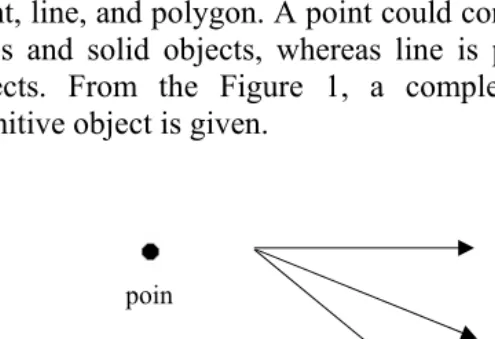
Any feature object appears in the real world is constructed by primitive object. The feature object could be a road, building, or just a simple traffic sign. They are represented by 3 kinds of primitives, i.e. point, line, and polygon. A point could construct the point itself, lines, faces and solid objects, whereas line is part of lines, faces or solid objects. From the Figure 1, a complete constructive model for primitive object is given.

Figure 1: Geospatial object

Any spatial object could be used to produce spatial analysis, e.g. 3D buffering model. From the Figure 1, the buffering models of each feature object are different according to the primitive that constructs them. The buffering model for primitive point is sphere, whereas the primitive line is a cylinder. Since nodes appear in the line segment, adding the point buffering model into the line buffer model becomes a necessity. Figure 2 shows the method to create a line buffering output.

construc poin

lin

surfac

poin

lin

polyg

polyg

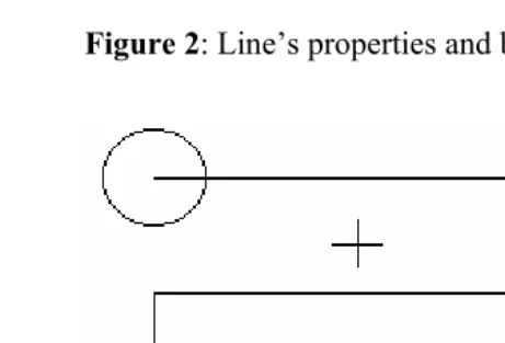
Refer to Figure 2, the buffering model for a line is a combination between spheres and cylinder. However, this combination creates an overlap segment (see Figure 3). This unnecessary segment is the internal segment and need to be removed. The complete modeling of line buffering object is discussed in Chen and Abdul-Rahman (2003). The third kind of primitive is polygon. A polygon feature is represented by some arc/node structure that determines an area’s boundary. With at least three or more nodes joining together consecutively and return to the starting node define a polygon. The buffering model for polygon is constructed by upper and lower faces (see Figure 4). However, to perform geometrically a buffering operation towards a polygon in three-dimensional space, the joined components of a single polygon need to be identified, which are the nodes, and edges. Therefore, the point and line buffering model should be considered in constructed polygon buffering model. The combination of point, line and face buffering model create internal segments that need to be removed. The complete modeling of polygon buffering object, including the removal of internal segment is discussed in Chen and Abdul-Rahman (2003).

point _edge line

x

z

y

x

z

y

x

z

Figure 2: Line’s properties and buffering model

Figure 3: Internal segment of line buffering model

Figure 4: Two buffering faces

Internal segment

polygon

y z

x

3.0 BUFFERING MODEL FOR SOLID OBJECT

A solid object constructed by faces could perform the buffering process. These faces connect each other, which shares the common vertices and lines, form a closed boundary. Therefore, the construction rule for a face is important in determine the internal and external aspect of a solid object. This is because the external aspect will be used in modeling the solid buffer zone. A series of points that construct a face in counter-clockwise direction is facing the external aspect; otherwise is internal. The main idea of differentiating the face’s aspect is to determine the upper and lower faces for polygon buffering (see Figure 5).

Figure 5: Upper and lower faces of polygon buffering model

Internal

External

(b) Counter clockwise

y z

x

The buffering layers are expanded upper and lower starting from the center of polygon, respective to the buffer length. Both of them should be parallel to the main polygon. To define these polygons buffer, the vector’s cross product is used. This vector produces a result that is perpendicular to the main polygon (v and u). For vectors u and v, the cross product is defined by (see Figure 6):

This can be written in a shorthand notation, which takes the form of a determinant (see Eq.1).

Figure 6: Vector (u x v)

Here, the (u x v) is always perpendicular to both u and v, with the orientation determined by the right-hand rule.

z y x z y x v v v u u u z y x v u / / /

u (Simplified

from Eq.1)

Some of the mathematics is illustrated below (refer to Figure 7). The vector u (A) and v (B) need to be compute in the early step (see

u v

Figure 7 and Equation 2 to 5). The purpose of computing those vectors is to find out the vector scale [|NX|, |NY|, |NZ|]. Later on the vector

scale are used to compute the point sets that form the polygon.

Figure 7: Vector for polygon P

OA x OB =

>

@

1

n =

ob ob oa oa Z Y Z Y (Eq.3) 2

n =

ob ob oa oa X Z X Z (Eq.4) 3

n =

o

AB =

>

@

o š

AB n n n

AB 1 2 3

r N x

x_{c o x} u

(Eq.8)

r N y

yc o y u

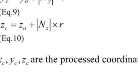
(Eq.9)

r N z

z_{c o z} u

(Eq.10)

where xc,yc,zcare the processed coordinates for the point C.

Figure 8: Upper polygon buffer CDE

y z

x

E C

D

A

O

Later on, point D and E will be calculated (see Figure 8) by using the same equations start from 2 to 10. From the Figure 7, three points (C, D, and E) create an upper layer of face for a polygon buffer model. Recall that a polygon is a combination of point, line and surface. The polygon buffering zone should implement point and line buffer model. After the upper polygon buffer is defined, the line (cylinders) and point (sphere) buffering objects need to be combined. However, the combination may produce internal segment between line and the polygon buffer. Same situation also occurs between point and line buffer. Therefore, the unnecessary internal segment needs to be removed.

To remove the internal segment between point and line buffer, the same approach as shown in Figure 2 is used. On the other hand, to remove the internal segment between line and polygon buffer, the approach is shown in Figure 9.

Figure 9: Combination of cylinder and surface buffer

View from above

O

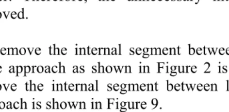
Main

y z

The cylinder and the point O from polygon (refer to the Figure 10), which is the point opposite to the cylinder and it is being a part of the main polygon. Either the third point that creates a polygon is O, O’, or even O” from the Figure 11, the representation remains the same as in Figure 10.

Figure 10: View from above

Figure 11: Method to remove internal segment

y z

x

A B C

O

External segment Internal segment

O

O’ O”

Cylinder

O

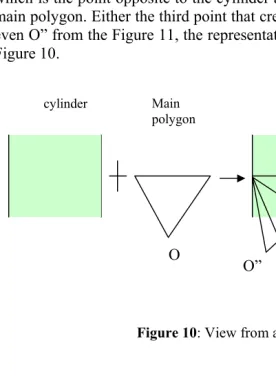
The cylinder is divided into two segments, which are the internal and external part. The main problem is to determine where the internal is and the external segment. Refer to Figure 12, d is the distant limit. The distance between cylinder segment and O (from the polygon) that exceeds d are identified as external segment.

Figure 12: Calculate distance between OA, OB, and OC

The distance of OA, and OC will be computed. Both of them are in the same situation because the surface of circle is perpendicular to the line AC. Points A and C are the upper and lower point of the circle (see Figure 12). Therefore, there is a condition that needs to be fulfilled in order to remove the internal segment of the cylinder. That is the distance of either OA or OC is the benchmark of that condition. If any distance from the circle to point O is less that OA or OC, then it should be the internal part of the cylinder and need to be removed. Finally, Figure 13 shows the processed result.

Internal segment

External segment

Figure 13: View from above

The remaining external segment (see Figure 13) will be used for another process, which the adjacent polygon buffer is combined (see Figure 14).

Figure 14: Final buffering zone

Processed cylinder Lower polygon buffer Upper polygon buffer

Main polygon

Buffering zone

4.0 EXPERIMENT AND DISCUSSIONS

In this project, the C++ language is used to create a software interface module called 3D Solid Buffering Tools. It is tested using simulated dataset. The representation of 3D solid buffering module / software will display the result using a commercial package called 3D Analyst. The input is in ASCII format and the result is presented in the shapefile (*.shp) format. Figure 15 shows the snap shots of the interface of the software, whereas Figure 16 and 17 present the output of the research.

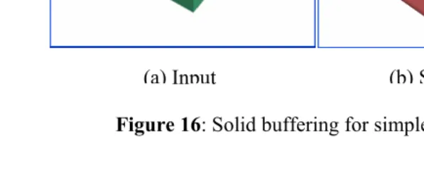
Figure 16: Solid buffering for simple object

Figure 17: Solid buffering for complex object

5.0 CONCLUDING REMARKS

The paper presents an approach for integrating all geometrical modeling of primitive buffering object in solving new spatial operations, i.e. 3D solid buffering. The integration is expected to be providing complete modeling for measurement-based 3D GIS analysis. The methodology was tested using C++ program and the result gives a positive output respected to the algorithm. Obviously, the initial outcomes of this experiment certainly will be utilized in the 3D GIS software development in the very near future, i.e. the 3D analytical operations.

REFERENCES

Chen, T.K., and Abdul-Rahman, A., (2003) “The Mathematics Of 3D Buffering For Simple Geospatial Primitives – An Effort To Realize 3D Buffering Operation For 3D GIS”. Geoinformation Science Journal, Vol. 3, No. 1, pp. 66-73.

Bernhardsen, Y., (1999) “Choosing a GIS in: Geographical Information Systems: Principles, Technical, Management and Applications”. John Wiley & Sons, Inc., 2nd edition, pp. 580-600.

Gaiani, M., Gamberini E. and Tonelli, G., (2001) “VR As Work Tool For Architectural & Archaeological Restoration: The Ancient Appian Way 3D Web Virtual GIS”. Virtual Systems and Multimedia, Proceedings. Seventh International Conference, 25-27 Oct. 2001, pp. 86 –95.