University of Windsor University of Windsor
Scholarship at UWindsor
Scholarship at UWindsor
Electronic Theses and Dissertations Theses, Dissertations, and Major Papers
2016
Identifying Suspended Accounts In Twitter
Identifying Suspended Accounts In Twitter
Xiutian Cui
University of Windsor
Follow this and additional works at: https://scholar.uwindsor.ca/etd
Recommended Citation Recommended Citation
Cui, Xiutian, "Identifying Suspended Accounts In Twitter" (2016). Electronic Theses and Dissertations. 5725.
https://scholar.uwindsor.ca/etd/5725
This online database contains the full-text of PhD dissertations and Masters’ theses of University of Windsor students from 1954 forward. These documents are made available for personal study and research purposes only, in accordance with the Canadian Copyright Act and the Creative Commons license—CC BY-NC-ND (Attribution, Non-Commercial, No Derivative Works). Under this license, works must always be attributed to the copyright holder (original author), cannot be used for any commercial purposes, and may not be altered. Any other use would require the permission of the copyright holder. Students may inquire about withdrawing their dissertation and/or thesis from this database. For additional inquiries, please contact the repository administrator via email
Identifying Suspended Accounts in
By
Xiutian Cui
A Thesis
Submitted to the Faculty of Graduate Studies through the School of Computer Science in Partial Fulfillment of the Requirements for
the Degree of Master of Science at the University of Windsor
Windsor, Ontario, Canada
2016
c
Identifying Suspended Accounts in Twitter
by
Xiutian Cui
APPROVED BY:
A. Hussein
Department of Mathematics and Statistics
L. Rueda
School of Computer Science
J. Lu, Advisor School of Computer Science
DECLARATION OF ORIGINALITY
I hereby certify that I am the sole author of this thesis and that no part of this
thesis has been published or submitted for publication.
I certify that, to the best of my knowledge, my thesis does not infringe upon
anyones copyright nor violate any proprietary rights and that any ideas, techniques,
quotations, or any other material from the work of other people included in my
thesis, published or otherwise, are fully acknowledged in accordance with the standard
referencing practices. Furthermore, to the extent that I have included copyrighted
material that surpasses the bounds of fair dealing within the meaning of the Canada
Copyright Act, I certify that I have obtained a written permission from the copyright
owner(s) to include such material(s) in my thesis and have included copies of such
copyright clearances to my appendix.
I declare that this is a true copy of my thesis, including any final revisions, as
approved by my thesis committee and the Graduate Studies office, and that this thesis
ABSTRACT
Large amount of Twitter accounts are suspended. Over five year period, about
14% accounts are terminated for reasons not specified explicitly by the service provider.
We collected about 120,000 suspended users, along with their tweets and social
re-lations. This thesis studies these suspended users, and compares them with normal
users in terms of their tweets.
We train classifiers to automatically predict whether a user will be suspended.
Three different kinds of features are used. We experimented using Nave Bayes
method, including Bernoulli (BNB) and multinomial (MNB) plus various feature
selection mechanisms (mutual information, chi square and point-wise mutual
informa-tion) and achieved F1=78%. To reduce the high dimensions, in our second approach
we use word2vec and doc2vec to represent each user with a vector of a shot and fixed
length and achieved F1 (73%) using SVM with RBF function kernel. Random forest
AKNOWLEDGEMENTS
I would like to present my gratitude to my supervisor Dr. Jianguo Lu for his
valuable assistance and support during the past three years. I cannot image I could
graduate without his help.
I also would like to express my appreciation to Dr. Abdulkadir Hussein, Dr. Luis
Rueda. Thank you all for your valuable comments and suggestions on this thesis.
Meanwhile, I would like to thank Zhang Yi for his great help on introducing
word2vec and doc2vec methods to me.
Finally, I want to thanks to my parents, my wife and my friends who give me
TABLE OF CONTENTS
DECLARATION OF ORIGINALITY III
ABSTRACT IV
AKNOWLEDGEMENTS V
LIST OF TABLES VII
LIST OF FIGURES IX
1 Introduction 1
2 Review of The Literature 4
2.1 Approaches . . . 5
2.2 Experiments . . . 9
2.3 Conclusion . . . 13
3 Dataset 15 4 Classification using N-gram Models 21 4.1 Naive Bayes Classifier . . . 21
4.1.1 Multinomial Naive Bayes Model . . . 22
4.1.2 Bernoulli Naive Bayes Model . . . 24
4.2 Evaluation and Confusion Matrix . . . 26
4.3 Feature Selection . . . 27
4.4 Experiments . . . 32
4.4.1 Feature Selection . . . 37
4.4.2 Conclusion . . . 52
5 Classification using word2vec and doc2vec 53 5.1 Experiments of word2vec . . . 53
5.2 Experiments of doc2vec . . . 57
6 Classification using bad words 60
7 Conclusion 65
References 65
APPENDIX A Classifiers used in experiments 70
APPENDIX B Classification results of word2vec and doc2vec 72
LIST OF TABLES
1 User Attributes in Benevenuto’s work . . . 6
2 User Attributes in Moh’s work . . . 7
3 Basic classification result in Benevenuto’s work . . . 10
4 Top 10 attributes in Benevenuto’s work . . . 11
5 Evaluation metrics for RIPPER algorithms with the different extended feature sets in Moh’s work . . . 11
6 Evaluation metrics for C4.5 algorithms with the different extended feature sets in Moh’s work . . . 12
7 Top 10 Information gain values for data set extended with RIPPER in Moh’s work. Added attributes are bold. . . 12
8 Top 10 χ2 values for data set extended with RIPPER in Moh’s work. Added attributes are bold. . . 13
9 Statistics of tweet dataset . . . 15
10 Token Types in Tweets . . . 17
11 Example of Unigram User Vectors . . . 23
12 2 Classes Confusion Matrix Example . . . 27
13 Meaning ofNcond . . . 29
14 Unigram Classification Result . . . 35
15 Bigram Classification Result . . . 36
16 Top 30 Unigram Features by MI. Terms in bold fonts are distinguished ones in suspended class. . . 39
17 Top 30 Unigram Features by PMI. Terms in bold fonts are distinguished ones in suspended class. . . 40
18 Top 30 Unigram Features by WAPMI. Terms in bold fonts are distin-guished ones in suspended class. . . 41
19 Top 30 Unigram Features byχ2. Terms in bold fonts are distinguished ones in suspended class. . . 42
20 Top 30 Bigram Features by MI. Terms in bold fonts are distinguished ones in suspended class. . . 43
22 Top 30 Bigram Features by WAPMI. Terms in bold fonts are
distin-guished ones in suspended class. . . 45
23 Top 30 Bigram Features by χ2. Terms in bold fonts are distinguished ones in suspended class. . . 46
24 Classification Results of Unigram on Different Feature Sizes . . . 50
25 Classification Results of Bigram on Different Feature Sizes . . . 51
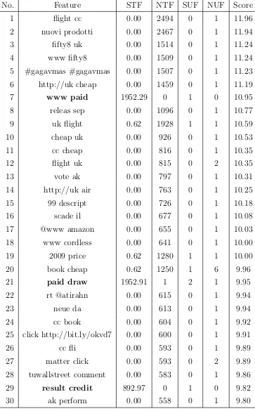
26 Top 10 Bad Words Sorted by Frequency in Suspended User Dataset,
STF = Suspended Token Frequency, NTF = Non-Suspended Token
Frequency, SUF = Suspended User Frequency, NUF = Non-Suspended
User Frequency . . . 60
27 Top 10 Hidden Bad Words, COS = Cosine Similarity between hidden
word and bad word, STF = Suspended Token Frequency, NTF =
Non-Suspended Token Frequency, SUF = Non-Suspended User Frequency, NUF
= Non-Suspended User Frequency . . . 63
LIST OF FIGURES
1 Tweet count distribution. Suspended users tend to have more tweets. 16
2 Frequency Distribution of Tokens . . . 18
3 Number of Tokens Per Tweet Distribution . . . 19
4 Distribution of Special Tokens . . . 20
5 Accuracy for BNB and MNB. Both unigram and bigram models are tested. . . 32
6 F1 for BNB and MNB. Both unigram and bigram models are tested. 33 7 Probabilities of all unigram feature in both classes . . . 34
8 Locations of Features selected by MI, PMI, WAPMI and χ2 . . . . . 48
9 Feature Size vs Accuracy and F1 . . . 49
10 Accuracy of classifiers on word2vec model . . . 56
11 F1 of classifiers on word2vec model . . . 56
12 Accuracy of classifiers on doc2vec model . . . 58
13 F1 of classifiers on doc2vec model . . . 58
14 Visualizations of Users . . . 59
15 The number of users who sent top bad words . . . 61
16 Bad words located by normalized token frequency . . . 62
CHAPTER 1
Introduction
Twitter is an online social network that provides users to send and read 140-short
messages named ”tweets”. It has already become one of the most-visited websites all
over the world. According to alexa.com, Twitter ranks 9th in the world top websites.
About 320 million users sending and reading tweets on Twitter every month and the
total number of registered users has already been over 1 billion [1]. By using tweets,
Twitter now has been considered as one of the fastest way to share information.
Obviously, it also attracts spammers.
Spammers are defined as those who send unsolicited tweets (spam), especially
ad-vertising tweets, as well as repeatedly sending mass duplicate messages [2, 3].
Spam-mers are usually generated by computers and works automatically. Twitter also faces
the same problem as the war between websites and spammers never ends. Twitter
will suspend users once they detect the behaviors of users abnormally, such as sending
spam or abusing tweets.
So it is important to analyze the suspended users to explore some methods to
pre-dict whether a user is spammer or not. Some approaches have been studied, including
machine learning technologies [4, 5], URL blacklists [6, 7], and some spammer traps
[8, 9].
However all these approaches faced some problems. Machine learning approaches
have already been widely used to detect spam email. Compared to classify spammers,
detecting spam email is easy because they can collect a huge number of spam email
and then train a classifier on it. But for detecting spammers, thing changed a lot
because we don’t have a large dataset of spammers. In the work of [4], they collected
only 355 spammers and the authors of [5] collected 77 spammers, which should be
considered too small to draw the whole picture of spammers on Twitter.
Second, machine learning methods are based on the features of spammers. These
1. INTRODUCTION
and user account attributes, such as how many friend or follower he has. However,
these features can be easily manipulated by spammers.
Other methods, such as blacklist or traps cannot work well all the time.
Spam-mers can easily avoid blacklists and traps by changing the approach of sending spam
message and the content because it is costless to generate new spammers.
In our work, we analyzed a large number of suspended users and proposed a
spammer prediction method. Unlike the previous work, we collected tweets from
113,347 suspended users during 5 years.
Based on this dataset, we combined the traditional machine learning technologies
and Paragraph Vector word embedding method to mapping tweets into vectors so
that we can predict whether a user will be suspended or not. We tried to classify
them by Naive Bayes classifier on n-gram models derived from the tweets. We also
tried 4 different feature selection methods, Mutual Information, Pointwise Mutual
In-formation, Weighted Averaged Pointwise Mutual Information andχ2. These methods can rank the features by score so that we can know which features are important and
which features are noise. By analyzing the classification results on different selected
features of these feature selection methods, we found that almost half of unigram
fea-tures are noise and 9/10 of bigram features are noise. After removing these features, we achieved 76.75 % accuracy and 78.54% F1 on using top 106 features selected by
WAPMI.
We also tried different word embedding methods to convert users into vectors. We
tried some classifiers on converted user vectors. When using SVM with RBF function
kernel, we achieved 73.28% accuracy and 73.39% F1 on 1,000 dimension user vector
trained by Paragraph Vector method. Although this result is lower compared to the
result of classification on feature selected n-gram models, this result is useful because
it only depends on a 1,000 dimension vectors.
After analyzing the characteristic of bad words using in suspended users, we found
the number of bad words using users is as twice larger as that number of normal users.
And we also introduced Badscore which can rank words by how close they are from
bad words.
The remainder of this thesis is structured as follows: In chapter II, we review
the previous works on spammer detection in OSNs. In chapter III, we address our
spammer detection method in detail. In chapter IV, we applied our experiments on
1. INTRODUCTION
together with classifications and feature selections on it. Finally, in chapter VI, we
CHAPTER 2
Review of The Literature
In this chapter, we will review some previews studies about suspended users on
twit-ter. By now, there are not many works analyzing the characteristic of suspended
users. The only work we found is proposed by Thomas et al [10]. They collected and
analyzed 1.1 million accounts suspended by Twitter. Their results show that 77%
spammers are suspended in the first day of their tweets, which makes them hard to
form relationships with normal users. Instead, 17% of them use hashtags and 53% of
them use mentions to reach out to normal users.
Other works were focusing on analyzing spammers and trying to find a way to
de-tecting spammers based on the extracted features [4, 11] or the relationships between
spammers [11, 5].
In 2010, Benevenuto et al. [4] addressed a study on the spammers who focused on
sending spam concluding the trending topics in Twitter. The main method they used
is to collect user profiles and tweets, then classify them into two groups, spammer and
non-spammer, by using Support Vector Machine (SVM). There are four steps in their
approach, crawling user data, labeling users, analyzing the characteristics of tweet
content and user behaviours and using a supervised classifier to identify spammers.
In the same year, Moh et al. [5] analyzed how much information gained from the
friends and followers of one user. They also proposed a learning process to determine
whether or not a user is spammer. There are two steps in this process. The first
step is to train a categorization algorithm to distinguish between spammers and
non-spammers on a set of basic user features. And the second step is to train a classifier
to generate new features, which depend on a user’s followers being spammers or
non-spammers.
In 2012, Ghosh et al. [11] analyzed over 40,000 spammer accounts suspended
by Twitter and found out that link farming is wide spread and that a majority
2. REVIEW OF THE LITERATURE
capitalists, who are themselves seeking to amass social capital and links by following
back anyone who follows them. And they proposed a ranking system, Collusionrank,
to penalize users from connecting to spammers.
2.1
Approaches
The works which are using machine learning methods to detecting spammers are using
nearly the same approaches. First they collected data from twitter, including tweets,
user account attributes and user relationships. After collecting, they will extract
features from these data and try to train classifiers on the extracted features to see
whether the features can represent the users and how well the classifiers work.
In order to classify the users into spammers and non-spammers, they used
su-pervised classifier. So they need to label one collection that contains spammers and
non-spammers. In this paper they focused on the users who sent the tweets about
trending topic, so they need to build one collection of users who sent topics of (1) the
Michael Jackson’s death, (2) Susan Boyle’s emergence, and (3) the hashtag
”#music-monday”. 8,207 users have been labeled manually, including 355 spammers and 7,852
non-spammers. They then randomly chose 710 non-spammers to reduce the number
of non-spammers. Thus, the total size of labeled collection is 1,065 users.
To use machine learning algorithms, they then identified the attributes of users.
The attributes are divided into two categories: content attributes and user behavior
attributes. Content attributes are the ones represented in what the users posted.
User behavior attributes are the properties of the users’ acting on Twitter. Both of
2. REVIEW OF THE LITERATURE
Category Attribute
Content Attributes
number of hashtags per number of words on
each tweet
number of URLs per words
number of words of each tweet
number of characters of each tweet
number of URLs on each tweet
number of hashtags on each tweet
number of numeric characters (i.e. 1,2,3)
that appear on the text, number of users
mentioned on each tweet
number of times the tweet has been retweeted
(counted by the presence of ”RT @username”
on the text)
User Behavior Attributes
number of followers
number of followees
fraction of followers per followees
age of the user account
number of times the user was mentioned
number of times the user was replied to
number of times the user replied someone
number of followees of the users followers
number tweets receveid from followees
existence of spam words on the users screen
name
the minimum, maximum, average, and
me-dian of the time between tweets
number of tweets posted per day and per
week
TABLE 1: User Attributes in Benevenuto’s work
After extracted features, they used SVM to classify user collections with the
2. REVIEW OF THE LITERATURE
used in their experiments is provided by libSVM. Each user in the user collection is
presented by a vector of values, which contains the attributes of this user. SVM will
first trains a model from the labeled user dataset, and then applies this model to the
classify the unknown users into two classes: spammers and non-spammers.
In the work [5], the authors used almost same idea of [4] but they introduced a
two steps categorization framework which can classify users not only based on the
content and user behavior attributes, and it also relies on the user’s friendships.
The first step of this framework is to train a model based on manually labelled user
collections. And then one extended attribute set will be generated for each user based
on the predictions provided by the first learner and the user’s position in the social
network. The learner will then be trained on this extended attribute set.
Category Attribute
Friend and Follower Attributes follower-friend ratio
Basic Attributes number of posts marked as favorites
Friend and Follower Attributes friends added per day
Friend and Follower Attributes followers added per day
Basic Attributes account is protected?
Basic Attributes updates per day
Basic Attributes has url?
Basic Attributes number of digits in account name
Friend and Follower Attributes reciprocity.
TABLE 2: User Attributes in Moh’s work
They extracted an attribute set for each user, which are shown in Table 2. Unlike
the previous works, the authors took the friend follower relationship into
consider-ation. They added some attributes which can measure the social network of users.
For example, the reciprocity is the rate of how likely a user follows his followers. In
practice, spammers tends to follow all the users who follows them. And they also
added some new basic attributes such as the number of digits in account name, which
has been proved useful in classification by Krause et al.[12].
2. REVIEW OF THE LITERATURE
first step using extracted attribute set. The authors modified the original formula.
trust metric = X
f ollowers
1
#users followed
They applied the following modifiers to this formula:
• legit accumulate only the values coming from users who are predicted to be
legitimate users
• capped accumulate only values coming from up to 200 users
• squared use #users followed×1#users followed instead of #users followed1
They tried the combinations of different classifiers on different steps. Then they
calculated the accuracy, precision, recall, F1, and finally draw a Receiver Operating
Characteristic Curve (ROC curve) to evaluate the test results of each combination.
Unlike these two papers which are focusing on detecting spammers on Twitter, the
work of [11] studied the link farm formed by spammers on Twitter. The dataset they
used includes a complete snapshot of the Twitter network and the complete history
of tweets posted by all users as of August 2009 [13]. To identify the spammers in this
dataset, they collected the user accounts which are suspended by Twitter. Although
the primary reason for suspension of accounts is spam-activity, the accounts which
are inactive for more than 6 months can also be suspended. One URL blacklist which
contains the most popular URLs in spam tweets has been constructed to confirm
that the suspended users are truly spammers. The authors fetched all the bit.ly or
tinyurl URLs that were posted by each of the 379,340 suspended accounts and found
that 41,352 suspended accounts had posted at least one shortened URL blacklisted
by either of these two shortening services. These suspended accounts were considered
to be spammers.
The authors studied how spammers acquire links to study link farm in Twitter by
analyzing the nodes following and followed by the 41,352 spammers. They defined the
nodes followed by a spammer as spam-targets and the nodes that follow a spammer
as spam-followers. Spam-targets who also follow the spammer are called targeted
followers. After computing the numbers of spammer-targets, spammer-followers and
targeted followers, they found out that the majority (82%) of spam-followers have
also been targeted by spammers. And targeted followers are likely to reciprocate most
2. REVIEW OF THE LITERATURE
links they created to the spammers) exhibited a reciprocation of 0.8 on average and
created 60% links to the spammers.
The authors also computed the Pagerank of each user in this dataset and found
out that by acquired large farm links from spammer followers, some of the rank of
spammers are very high, 7 spammers rank within the top 10,000 (0.018% of all users)
304 and 2,131 spammers rank within the top 100,000 (0.18% of all users) and 1 million
(1.8% of all users) users according to Pagerank, respectively.
The authors then analyzed the users who willing to reciprocate links from arbitrary
users and the reason why they need to farm links. They plotted how the probability
of a user reciprocating to a link from spammers varies with the user’s indegree and
found out that the lay users, who have low indegree, rarely respond to spammers. On
the other hand, users with high indegree value are more likely to follower a spammer.
And the authors also found out that the top link farmers (top 100,000
spam-followers) sometimes are active contributors instead of spammers. The motivating
factor for such users might be the desire to acquire social capital and thereby,
influ-ence.
The authors proposed Collusionrank, a Pagerank-like approach, to combat link
farming in Twitter. Collusionrank algorithm can also be combined with any ranking
strategy used to identify reputed users, in order to filter out users who gain high
ranks by means of link farming. To evaluating Collusionrank, the authors computed
the Collusionrank scores of all users in the Twitter social network, considering as the
set of identified spammers S, a randomly selected subset of 600 out of the 41,352 spammers.
The result of evaluation showed the effect of ranking spammers of Collusionrank
is great. While more than 40% of the 41,352 spammers appear within the top 20%
positions in Pagerank, 94% of them are demoted to the last 10% positions in
Collu-sionrank. Even when only a small set of 600 known spammers is used, this approach
selectively filtered out from the top positions of Pagerank, most of the unidentified
spammers and social capitalists who follow a large number of spammers.
2.2
Experiments
We compare the results from works [4, 5], which are trying to detect spammers based
2. REVIEW OF THE LITERATURE
In [4], they collected all user IDs ranging from 0 to 80 million since August 2009,
which have been considered as all users on Twitter since there is no single user in the
collected data had a link to one user whose ID is greater than 80 million. Finally they
collected 54,981,152 used accounts that were connected to each other by 1,963,263,821
social links, together with 1,755,925,520 tweets. Among those users, there are 8%
accounts were set private and were ignored. The detail description of this dataset can
be found on their project homepage[14].
They then trained SVM based on the features listed in Table 1. Table 3 shows
the confusion matrix of classification result. About 70% of spammers and 96% of
non-spammers were correctly classified. The Micro-F1 (which is calculated by first
computing global precision and recall values for all classes, and then calculating F1)
is 87.6 %.
Predicted
Spammer Non-spammers
True Spammer 70.1% 29.9%
Non-spammer 3.6% 96.4%
TABLE 3: Basic classification result in Benevenuto’s work
To reduce the misclassifying of non-spammers, the authors used two approaches.
First is to adjust J parameter in SVM. In SVM, J parameter can be used to give
priority to one class over the other. With the varying of J, the rate of correctness of
classify can be increased to 81.3% (J = 5), with the misclassifying of legitimate users
has been increased to 17.9%.
The second approach they used is to reduce the size of attributes set. By sorting
the attributes by their importance, the authors can remove the non-important
at-tribute and give more weight to the important ones. They used two feature selection
methods, information gain and χ2, which are available in Weka. The results of these two methods are similar and the top 10 attributes in result are same. Table 4 shows
the top 10 result of feature selection. And the result of classification when just using
top 10 attributes instead of all attributes shows that top 10 attributes are enough to
2. REVIEW OF THE LITERATURE
Rank Attribute
1 fraction of tweets with URLs
2 age of the user account
3 average number of URLs per tweet
4 fraction of followers per followees
5 fraction of tweets the user had replied
6 number of tweets the user replied
7 number of tweets the user receive a reply
8 number of followees
9 number of followers
10 average number of hashtags per tweet
TABLE 4: Top 10 attributes in Benevenuto’s work
The authors of [5] collected the account names of spammers using the web page
twitspam.org, where users can submit the names of suspected spammers. Another
part of spammers were added by the authors during they collected data. They
ob-tained non-spammers from the users they followed. In total they collected one dataset
that contains 77 spammers and 155 non-spammers. And for each user in this dataset,
they also collected the information on up to 200 of their followers.
For there are two steps in classification, the authors tried different combination of
classifiers. Then they calculated the accuracy, precision, recall, F1, and finally draw
a Receiver Operating Characteristic Curve (ROC curve) to evaluate the test results
of each combination. Table 5 and Table 6 show the evaluation metrics for RIPPER
algorithm and C4.5 algorithm.
Metric basic basic+peer peer basic+trust all features
Precision 0.79 0.80 0.75 0.88 0.84
Recall 0.84 0.83 0.71 0.85 0.85
F1 0.81 0.81 0.73 0.87 0.84
Accuracy 0.87 0.87 0.82 0.91 0.90
TABLE 5: Evaluation metrics for RIPPER algorithms with the different extended
2. REVIEW OF THE LITERATURE
Metric basic basic+peer peer basic+trust all features
Precision 0.80 0.81 0.72 0.85 0.86
Recall 0.85 0.79 0.67 0.85 0.86
F1 0.83 0.80 0.69 0.85 0.86
Accuracy 0.88 0.87 0.80 0.90 0.90
TABLE 6: Evaluation metrics for C4.5 algorithms with the different extended feature
sets in Moh’s work
The authors also tried to measure the information provided by each features. To
do so, the authors calculated the information gain and the chi square values for each
feature in extended feature set.
The authors claimed that using RIPPER in two steps achieved the best
perfor-mance among the combinations of classifiers. And top 10 features ranked by
infor-mation gain and chi square value is shown in Table. 7 and Table. 8.
Attribute Information gain
spammers to legit followers 0.48
friend-follower ratio 0.35
friends per day 0.34
trust metric legit. 0.34
trust metric legit. capped 0.29
trust metric 0.29
friend-follower average for friends 0.27
average protected for followers 0.25
trust metric legit. square 0.24
average protected for friends 0.24
TABLE 7: Top 10 Information gain values for data set extended with RIPPER in
2. REVIEW OF THE LITERATURE
Attribute Chi square value
spammers to legit followers 128.68
friends per day 106.72
trust metric legit. 105.49
friend-follower ratio 101.23
trust metric legit. capped 94.8697
trust metric 88.78
friend-follower average for friends 81.54
average protected for followers 80.57
trust metric legit. square 79.93
trust metric legit. square capped 74.99
TABLE 8: Top 10 χ2 values for data set extended with RIPPER in Moh’s work. Added attributes are bold.
2.3
Conclusion
Previous works studied a lot of spammers and trained classifier to detect spammers on
Twitter. They found some extracted features based on the content attributes, account
attributes and relationships of users can identify whether users are spammers. The
classifiers they trained based on these features achieved a great results.
They also tried analyzing the structure in suspended users and behaviors of
sus-pended users. They found that the sussus-pended users lack of ways of form the social
relationship with normal users, so they can only rely on mentions or hashtags to
contact with normal users.
However, these works still have their own problems. First is the way they collected
the spammers’ data. The authors of [4] used the data of users who sent the tweets
about trending topics, the authors of [5] used the data from twitspam.org and the
authors of [11] used the data of suspended users who sent tweets including shortened
URL. All the approaches should be considered can only show one part of suspended
users. According to the analysis of our dataset, there are many suspended users
who didn’t send any tweets about trending topics or including shortened URL. And
twitspam.org cannot provide a full list of suspended users because the users on that
2. REVIEW OF THE LITERATURE
of all users who were suspended after 5 years, which can provide more information
and full characteristics of suspended users.
Second problem is when analyzing the behaviors of suspended users, they didn’t
use full text of tweets. Whether users should be suspended, firstly and mainly is
depending on the tweets they sent. So It is really significant to analyze the tweets
of suspended users. But in their works, they only used some content attributes, such
as number of hashtags per words or number of URLs per words. Such attributes can
be easily manipulated by spammers by simply increasing the percentage of normal
tweets in all tweets they send. What’s more, shortened URL can be hidden by just
remove http protocal header so that the blacklist system cannot detect the tweets
containing urls.
Our work tried to used full text of tweets and large dataset of suspended users to
CHAPTER 3
Dataset
The dataset we used in our experiments is collected by T. Xu et al [15]. There
are 3,117,750 users’ profile, social relations and tweets in this dataset. They used
4 machines with whitelisted IPs to crawl data by Twitter API. The crawling was
first started with the most popular 20 users reported in [16] and then used snowball
crawling strategy to crawl other users. The crawling period was from Mar. 6 to Apr.
2, 2010.
5 years later, 113,347 users in these dataset were suspended by Twitter. We
randomly sampled 10% (11,334) of suspended users and the same number of normal
users who are not in the suspended user set in the original dataset and combined them
as our dataset. For each user in our dataset, we used regular expression to extract the
tweets from the original dataset, resulting in 4,518,074 tweets from suspended users
and 2,588,032 tweets from non-suspended users. The statistics of tweets of suspended
and normal users are summarized in Table 9.
Suspended Users Non-Suspended Users
# Users 11,334 11,334
# Tweets 4,518,074 2,588,032
# Tokens 30,366,927 18,778,909
Vocabulary (# Unique Token) 1,489,281 1,089,437
Average Tweets Length 6.72 7.25
Average URL Rate 12.14% 11.90%
Average Mention Rate 27.43 % 23.39%
Average Hashtag Rate 4.32% 3.89%
TABLE 9: Statistics of tweet dataset
We analyzed some properties of our dataset and compared the results to show the
3. DATASET
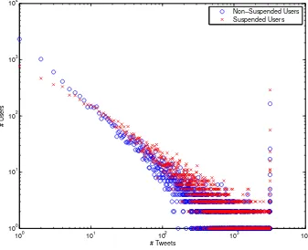
number of tweets of each user. Fig. 1 shows the distribution the count of tweets from
users. They follow power laws for both suspended and normal users. Most users have
one or two tweets. Among suspended users, there are close to one thousand users who
send tweets only once, while there are more than two thousand users who send tweets
only once. Because of the scarcity of the text, these users will be difficult to classify.
There are also some users who sent tweets close to two thousands. The maximal
tweet number is two thousand, because the data are crawled with two thousand as a
limit. Such distributions differ from most text corpora – in corpora such as Reuters
data sets, document lengths follow normal or log-normal distributions, where most
documents have medium length. In our data, most documents have very few tweets.
This will make classification more challenging.
We can also find that suspended users tend to send more tweets, as the slopes
intersect around 10 tweets. There are more suspended users who send tweets more
than 10 times. In average, suspended user send 398.63 tweets, while normal users
send only 228.34 tweets in average.
100 101 102 103 104
100 101 102 103 104
# Tweets
# Users
Non−Suspended Users Suspended Users
FIGURE 1: Tweet count distribution. Suspended users tend to have more tweets.
We then moved closer to look at the details of tweets by tokenizing the tweets
3. DATASET
Table 10. We first used regular expression to split every tweet into tokens and then
normalized the word tokens. Tokenization in tweets are different from normal text,
because we need to keep track of urls, hashtags, and user mentioning.
Token Type Description Regular Expression Example
Words
contains
characters or
digit numbers
[ A-Za-z0-9]+ Sample
Shortened URL
an url should
start with http
or https
http://[ A-Za-z0-9\./]+ http://t.co/ABcd123
Mention Users
used to mention
other user by
their username
@[ A-Za-z0-9]+ @twitter
Hashtags
used to mark
keywords or
topics in a tweet
#[ A-Za-z0-9]+ #spam
TABLE 10: Token Types in Tweets
After tokenizing, we turn all the tokens in lower case, then remove stop words
using the stop word list from [17]. Stemming is also carried out using Porter2
stem-ming algorithms [18]. the program used in the experiment is downloaded from [19].
Stemming converts words into the root form so that different derived words from the
same root will be treated as the same one. For example, after stemming ”making”
and ”made”, they will be converted into the root form ”make”.
After normalization, suspended user class contains total number of 30,366,927
tokens. Among them 1,489,281 are distinct. Normal users contain 18,778,909
to-kens, 1,089,437 are distinct. These two vocabularies share 285,052 unique tokens in
common.
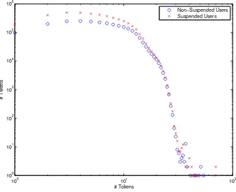
The frequency distribution of tokens is plotted in Fig. 2. In both classes, the
distributions follow Zipf’s law as expected. There are very large number of terms
that occur only once or twice. At the same time, there are also lot of popular terms
that occur frequently. The slope is roughly two, consistent with most other text
corpora. The counts for suspended class is higher because each user has more tweets.
3. DATASET
100 101 102 103 104 105 106
100 101 102 103 104 105 106 107
Token Frequency
# Tokens
Non−Suspended Users Suspended Users
FIGURE 2: Frequency Distribution of Tokens
distribution of number of tokens in tweet. The average number of tokens in tweet
from suspended users is 6.72 and that from non-suspended users is 7.25. Fig. 3
shows the distribution of number of tokens in tweet. This figure illustrates why the
number of tweets from suspended users is larger than that of non-suspended users.
This larger part is because of the number of short tweets (number of tokens < 10) from suspended users is much larger than that of normal users. This result and the
result of tweets distribution can draw a conclusion that suspended users tend to send
large number of short tweets. This conclusion can match our assumption that the
main reason of suspending is because these users sending tweets against Twitter Rule,
including abusive actives and spamming activities. Both of these two type of tweets
are usually short on length while large on number to either abusing normal users or
attracting normal users.
Among these tokens, URL, Mention and Hashtag are more special than the other
tokens. The probabilities of occurrences of these 3 types of tokens have been plotted
in Fig. 4. We excepted that the probabilities of these 3 types of tokens are very
different between suspended users and non-suspended users as the previous studies
3. DATASET
100 101 102
100 101 102 103 104 105 106
# Tokens
# Tweets
Non−Suspended Users Suspended Users
FIGURE 3: Number of Tokens Per Tweet Distribution
suspended and non-suspended users. The average of URL rate, mention rate and
hashtag rate don’t vary too much between these two dataset. The average rates are
listed in Tabel 9.
What we can conclude from the analysis of suspended user dataset and
non-suspended user dataset is that when using large, random sampled non-suspended user
dataset instead of the target focusing crawling dataset in the previous studies, it is
hard to classify users based on the rates of special tokens. The collecting methods that
previous papers used cannot reveal the characteristics of suspending users because
3. DATASET
0 0.2 0.4 0.6 0.8 1
10−3 10−2 10−1 100
Probability of URL
User Percentage
URL
0 0.2 0.4 0.6 0.8 1
10−3 10−2 10−1 100
Probability of Mention
User Percentage
Mention
0 0.2 0.4 0.6 0.8 1
10−4 10−3 10−2 10−1 100
Probability of Hashtag
User Percentage
Hashtag
Suspended Users
Non−Suspended Users
FIGURE 4: Distribution of Special Tokens
Summary we collected tweets of 113,347 suspended users, and tweets of equal
number of normal users to avoid the complexity arising from imbalanced data. there
are a few difference from other text corpora. In tokenization, we need to retain urls,
mentioning, and hashtags. Document lengths follow power law instead of lognormal
distributions. There are many very short documents. This will make classifications
CHAPTER 4
Classification using N-gram
Models
4.1
Naive Bayes Classifier
In this approach, all the terms are potential features, although we will also need to
select from them for efficiency and performance consideration. This can be further
divided into at least two models, the unigram model and bigram model.
In the unigram model, a document (i.e., all the tweets of a user) is treated as a
bag-of-words. The word position information is discarded, while the count of word
occurrences are retained. This model has the disadvantage that the order of the words
are no longer relevant.
Thus, n-gram models are introduced. In n-gram models, a document is represented
as a set of n-grams, where an n-gram is a consecutive sequence of terms with length n.
Although in theory we can use tri-gram, or even 4-gram, in practice bigrams are most
often used. Unlike unigram model, bigram model can carry a little information of
word ordering. This is because when converting tweets into bigrams, the consecutive
two words will be converted into one bigram.
In both unigram and bigram models, the feature size is very large, in the order
of 106. Most classification methods can not run on such high dimension. Hence we
experiment with Naive Bayes classifiers.
There are two different Naive Bayes classifiers, i.e., Multinomial Naive Bayes
Model (MNB) and Bernoulli Naive Bayes Model (BNB). The difference between
these two models is that Multinomial Model takes the number of occurrences into
consideration while Bernoulli Model only considers weather a term occurs in user’s
4. CLASSIFICATION USING N-GRAM MODELS
These two models are based on Bayes’ theorem [20],
P(A|B) = P(B|A)P(A)
P(B)
where P(A) and P(B) are the probabilities of A and B; P(A|B) is a conditional probability of observing event A given that B is true; P(B|A) is the probability of observing event B given that A is true.
Hence, the probability of a user being suspended can be computed by,
P(cs|w1, w2, ..., wn) =
P(cs)P(w1|w2, ...wn, cs)P(w2|w3, ...wn, cs)...P(wn|cs)P(cs)
P(w1, w2, ..., wn)
where cs is the event that user is suspended and wk is the kth word in tweets from this user. After training, P(w1, w2, ..., wn) will be constant. So the probability
P(cs|w1, w2, ..., wn) is only depended on the prior probability P(cs) and the likeli-hood P(cs)P(w1|w2, ...wn, cs)P(w2|w3, ...wn, cs)...P(wn|cs). If using the assumption that the probability of each word are independent, which means the occurrences of
words are not replying on others, P(wi|w2, ...wn, cs) = P(wi|cs), we can simplify the formula based on this assumption,
P(cs|w1, w2, ..., wn)∝P(cs) Y
1≤k≤nd
P(tk|c)
So the classification result can be comparison of classes c which can maximize the probability P(c|w1, w2, ..., wn).
4.1.1
Multinomial Naive Bayes Model
In Multinomial Model, the class of a user can be determined by the following formula:
c= arg max c∈C
P(c) Y 1≤k≤nd
P(tk|c)
wherecis the classified class of this user, C contains two classes: Suspended User and Normal User,nd is the number of tokens in userd,P(c) is the probability of this user occurring in classcand P(tk|c) is the probability of tokentk occurring in a user of class c.
Users will be converted into vectors by their tweets under MNB. For example,
there are two users whose tweets listed below:
4. CLASSIFICATION USING N-GRAM MODELS
(a) This is a sample tweet. see this: http://bitly.com/abc @user
(b) This is another tweet. #somehashtag
2. User 2
(a) This tweet contains some different words.
will be converted into two vectors by using unigram model:
S1 = (1,1,1,3,1,1,1,2,2,0,0,0,0)
S2 = (0,0,0,0,1,0,0,0,1,1,1,1,1)
The vocabulary and converting details are shown in Table. 11. All the words in this
table are normalized so that they might be different from the original words in the
tweets.
Unigram # in User 1 # in User 2
#somehashtag 1 0
@user 1 0
anoth 1 0
see 1 0
this 3 1
sampl 1 0
http://bitly.com/abc 1 0
a 1 0
is 2 0
tweet 2 1
word 0 1
differ 0 1
some 0 1
contain 0 1
TABLE 11: Example of Unigram User Vectors
We estimated P(c) and P(tk|c) by Maximum Likelihood Estimate (MLE).
P(c) = Nc
N P(tk|c) =
Tct
4. CLASSIFICATION USING N-GRAM MODELS
where Nc is the number of users in this class c, N is the total number of users,
Tct is the number of occurrences of token t in class c and Tc is the total number of tokens that occur in classc. In our cases, the number of suspended users and normal users are the same, so P(c) = 0.5. Laplace smoothing was used here to eliminate the condition that the number of token occurrence is 0, which is to add 1 to each term
occurrences in the formula of P(tk|c):
P(tk|c) =
Tct+ 1
Tc+|V|
where |V| is the size of vocabulary. Algorithm 1 illustrates how we train the Multi-nomial Model and use it to classify a user.
Procedure 1 Train Multinomial Naive Bayes Model and Classify Users
Input: labelled user feature map setU, class setC
Output: multinomial naive bayes modelM N B M odel
1: procedureTRAIN MULTINOMIAL NB MODEL
2: V ←EXTRACT TOKENS(U)
3: forc∈Cdo
4: Nc←COUNT USER IN CLASS(U,c)
5: M N B M odel.clsP rob[c]←log(Nc
|U|) 6: fort∈V do
7: Tct←COUNT TOKENS IN CLASS(U,c,t)
8: Tc←COUNT TOKENS(U,c)
9: M N B M odel.clsF eatureP rob[c][t]←log(Tct+1
Tc+|V|) 10: end for
11: end for
12: returnM N B M odel
13: end procedure
Input: trained multinomial naive bayes modelM N B M odel, unclassified user feature mapu, class setC
Output: classified classcforu
1: procedureCLASSIFY BY MULTINOMIAL NB MODEL
2: forc∈Cdo
3: score[c]+ =M N B M odel.clsP rob[c]
4: fork, v∈udo
5: ifk∈M N B M odel.clsF eatureP rob[c]then
6: score[c]+ =M N B M odel.clsF eatureP rob[c][k]∗v
7: end if
8: end for
9: end for
10: returnarg maxc∈Cscore[c]
11: end procedure
4.1.2
Bernoulli Naive Bayes Model
Bernoulli Naive Bayes Model, on the other hand, uses the boolean model in which
4. CLASSIFICATION USING N-GRAM MODELS
in the tweets this user posted. The value of a token is 1 if the token occurs, otherwise
it is 0. For example, the previous users will be converted into:
S1 = (1,1,1,1,1,1,1,1,1,0,0,0,0)
S2 = (0,0,0,0,1,0,0,0,1,1,1,1,1) The formula of classifying a user under Bernoulli Model is,
c= arg max c∈C
P(c) Y 1≤k≤|V|
P(tk|c)xi(1−P(tk|c)1−xi)
wherexiis the boolean expression of whether tokenioccurs in the tweets of this user. The P(c) and P(tk|c) can be estimated under Bernoulli Model like this,
P(c) = Nc
N P(tk|c) =
Nct
Nc
where Nct is the number of users in class c whose tweets contain token t. We also smoothed the formula of P(tk|c):
P(tk|c) =
Nct+ 1
Nc+ 2
4. CLASSIFICATION USING N-GRAM MODELS
Procedure 2 Train Bernoulli Naive Bayes Model and Classify Users
Input: labelled user feature map setU, class setC
Output: bernoulli naive bayes modelBN B M odel
1: procedureTRAIN BERNOULLI NB MODEL
2: BN B M odel.V ←EXTRACT TOKENS(U)
3: forc∈Cdo
4: Nc←COUNT USER IN CLASS(U,c)
5: M N B M odel.clsP rob[c]←log(Nc
|U|) 6: fort∈BN B M odel.V do
7: Nct←COUNT USERS CONTAINING TOKEN IN CLASS(U,c,t)
8: BN B M odel.clsF eatureP rob[c][t]←Nct+1
Nc+2
9: end for
10: end for
11: returnBN B M odel
12: end procedure
Input: trained bernoulli naive bayes modelBN B M odel, unclassified user feature mapu, class setC
Output: classified classcforu
1: procedureCLASSIFY BY BERNOULLI NB MODEL
2: forc∈Cdo
3: score[c]+ =BN B M odel.clsP rob[c]
4: fort∈BN B M odel.V do
5: ift∈u.keysthen
6: score[c]+ =log(BN B M odel.clsF eatureP rob[c][t])
7: else
8: score[c]+ =log(1−BN B M odel.clsF eatureP rob[c][t])
9: end if
10: end for
11: end for
12: returnarg maxc∈Cscore[c]
13: end procedure
4.2
Evaluation and Confusion Matrix
To evaluate the result of classification, we used N-fold cross validation. First divided
the dataset into N folds, which are same size. And then run N times of validation on
the datasets that one fold is used as test dataset and other folds are used as training
dataset.
We used confusion matrix to visualize the result of cross validation. Table 12
shows the confusion matrix of 2 classes cross validation result, TP represents the
number of suspended users that are classified as suspended users, FP represents the
number of suspended users that are classified as normal users, FP represents the
number of normal users that are classified as suspended users and FN represents the
number of normal users that are classified as normal users. We can compute accuracy
4. CLASSIFICATION USING N-GRAM MODELS
Classified
Suspended User Normal User
Actual Class Suspended User TP FN
Normal User FP TN
TABLE 12: 2 Classes Confusion Matrix Example
Accuracy= T P +T N
T P +F P +F N +T N Recall= T P
T P +F N P recision= T P
T P +F P
F1 = 2× P recision+Recall
P recision×Recall
These 4 parameters can measure the result of classification. Accuracy can measure
the total accuracy rate of classification of suspended users and non-suspended users;
recall shows the rate of how many users who are actually should be suspended will be
suspended; precision can measure the precision of classifier on predicting suspending;
F1 illustrates the overall performance of this classifier.
4.3
Feature Selection
When using n-gram language model, the main problems we face is the huge size of
feature set, leading to a lot of time spending on training and testing. We can use
feature selection algorithms to reduce the size of feature set. Another benefit we can
get is that using feature selection can remove the irrelevant features, also known as
noise features.
To remove the noise features and improve the result of classification, we used
several feature selection algorithms: Mutual Information (MI), Pointwise Mutual
Information (PMI), Weighted Average Pointwise Mutual Information (WAPMI) and
4. CLASSIFICATION USING N-GRAM MODELS
Mutual Information, which is also called Information Gain, can measure how much
information contribution of a token during the classification. We computed Mutual
Information by the following formula,
M I(t, c) = X et∈1,0
X
ec∈1,0
P(U =et, C =ec) log2
P(U =et, C =ec)
P(U =et)P(C =ec)
whereetis a boolean variable representing whether termt occurs in user’s tweets and
ecis a boolean variable that represents whether user is in classc. In our experiments, we let ec = 1 represent the user is suspended and ec = 0 represent user is normal user. We can also use MLE to estimate the probabilities P(U = et, C =ec), P(U =
et), P(C =ec):
ˆ
P(U =et, C =ec) =
Netec
N
ˆ
P(U =et) =
Net
N
ˆ
P(C =ec) =
Nec
N
where Ncond is the number of users that match condition cond. For example N11 is the number of users that match two condition: toccurs in these users’ tweets and all of these users are suspended. The formula of mutual information can be converted
by using MLE estimation
M I(t, c) = N11
N log2
N N11
N1.N.1
+N01
N log2
N N01
N0.N.1 + N10
N log2
N N10
N1.N.0
+N00
N log2
N N00
N0.N.0
The variable meanings in this formula are listed in Table 13. We applied
4. CLASSIFICATION USING N-GRAM MODELS
Variable Meaning
N11 the number of suspended users whose tweets contain term t
N01 the number of suspended users whose tweets don’t contain term t
N10 the number of non-suspended users whose tweets contain term t
N00 the number of non-suspended users whose tweets don’t contain term t
N1. the number of users whose tweets contain term t
N.1 the number of suspended users
N0. the number of users whose tweet don’t contain term t
N.0 the number of non-suspended users
N the number of total users in both suspended user set and normal user set TABLE 13: Meaning ofNcond
However, when the token frequency is imbalanced between suspended users and
non-suspended users, although the number of suspended users (N.1) and the number of non-suspended users are similar, we will still be facing the problem that the feature
selection method will have more probability to select the features from suspended
users than select from non-suspended users. We will show the result in experiment
section about this. In order to solve this problem, we used token frequency instead
of number of users. The definitions of N11 and N10, which now are the frequency of this feature occurring in suspended user dataset and the frequency of this feature
occurring in non-suspended user dataset, remain similar to the original definitions.
And we can compute N01 and N00 by,
N01 =N.1−N11
N00 =N.0−N10
where N.1 is the sum up of total feature frequency in suspended users and N.0 is the sump up of total feature frequency in non-suspended users.
4. CLASSIFICATION USING N-GRAM MODELS
E11=N ×P(t)×P(c) =
N1.N.1
N E10=N ×P(t)×(1−P(c)) =
N1.N.0
N E01=N ×(1−P(t))×P(c) =
N0.N.1
N E00=N ×(1−P(t))×(1−P(c)) =
N0.N.0
N
So the formula of MI can be simplified to,
M I(t, c) = X et∈{0,1}
X
ec∈{0,1}
Netec
N log2 Netec
Eetec
We can easily figure out when 1) the frequency of this feature is high in both
suspended users and non-suspended users; 2) the frequency of this feature is different
between suspended users and non-suspended users slightly, MI will give this feature
a high score. The first condition can prove to increase P(U =et, C =ec) =Netct/N
and the second condition can make Netec
Eetec increase. So together this feature will be selected by MI.
Pointwise Mutual Information is a little different from MI because MI is focusing
on the average of all the events while PMI only is focusing on the single events:
P M I(t, c) = X ec∈{0,1}
|log2 P(U =etC =ec)
P(U =et)P(C =ec)
|
= X
ec∈{0,1}
|log2 N1ec
E1ec
|
Compared to the formula of MI, PMI only depends on the frequency difference
between suspended users and non-suspended users, which is measure by ne. So unlike
that MI will select those popular features in both datasets, PMI will focus on the rare
words instead.
Although MI and PMI can measure how strong the relationship between feature
and the class is, there are 2 problems in them. First is that they all treat the
fea-tures as independent random variables when they estimate the probability of feafea-tures
occurring in tweets. However, in real tweets the features (words) are not
indepen-dent. This kind of estimation loses the relationship between features. Second is that
4. CLASSIFICATION USING N-GRAM MODELS
the tweets, the conditional probability usually is computed by merging all of tweets
together as a large tweet. This will give the words in longer tweet a larger weight.
In 2005, K Schneider et al [21] proposed a weighted algorithm for computing
point-wise mutual information. They added the weight to pointpoint-wise mutual information to
reduce the bias of giving longer tweet large score. WAPMI of token t in class c can be computed by,
WAPMI(t, c) =X c∈C
X
d∈Dc
αdp(t|d) log2
p(t, c)
p(t)p(c)
whered is the tweet that contains tokent,Dc is the set of tweets in classc. p(t|d) is the conditional probability oft, which is computed by,
p(t|d) = n(t, d)
|d|
where n(t, d) is the frequency of token t occurring in tweet d and |d| is the total size of tweet d.
αdis the weight of tokent. The authors gave 3 different weighting method in [21], which are:
• αd =p(c)× |d|/Pd∈Dc|d|. Each tweet has been given a weight correlation to
their length|d|.
• αd= 1/Pc∈C|c|. This will give tweets in the same class an equal weight.
• αd= 1/(|Dc| × |C|). This will give equal weight to the classes by normalization by class size.
χ2 is another feature selection method which can measure the relationship between the token and class. The lower the χ2 score is, the token and class are more inde-pendent to each other. χ2 can be computed by the deviation between the excepted frequency and the observed frequency of tokent in classc.
χ2(t, c) = X et∈{0,1}
X
ec∈{0,1}
(Netec−Eetec)
2
Eetec
4. CLASSIFICATION USING N-GRAM MODELS
4.4
Experiments
We first tried unigram and bigram model using two different Naive Bayes
classifi-cation, Multinomial and Bernoulli models. All the tweets have already been split
by regular expression. Then stop words have been removed and all the tokens have
been normalized in the previous section. So the only thing we need to do to convert
tweets into vectors is to generate unigrams and bigrams and count the frequency. For
Multinomial model, each location in the vector is the frequency of the gram of this
location; for Bernoulli model, each location in the vector is 1 if the gram occurring
in the tweets of this user. The dimension of word vectors using unigram is 2,293,666
and the dimension of word vectors using bigram is 17,485,806.
All these processes have been done by C++ so that we can manually control the
memory and achieve a better performance. When implementing, we used a
feature-frequency dictionary in memory because the matrix of user vectors are so sparse.
We tested Multinomial Naive Bayes classifier and Bernoulli Naive Bayes classifier on
processed dataset. Table 14 and 15 show the result of 10-fold cross validation of
these two classification models on unigram and bigram model. Fig. 5 and 6 show the
variant of classifiers during 10 runs.
0.54 0.55 0.56 0.57 0.58 0.59
MNB+Unigram BNB+Unigram MNB+Bigram BNB+Bigram
Accuracy
FIGURE 5: Accuracy for BNB and MNB. Both unigram and bigram models are
4. CLASSIFICATION USING N-GRAM MODELS
0.3 0.35 0.4 0.45 0.5 0.55 0.6 0.65 0.7
MNB+Unigram BNB+Unigram MNB+Bigram BNB+Bigram
F1
FIGURE 6: F1 for BNB and MNB. Both unigram and bigram models are tested.
The tables show that bigram model outperforms unigram model when using MNB
classifier both on accuracy and F1. However the results of MNB are not good enough.
This is because the probabilities of grams in both classes is similar. Fig. 7 shows the
comparison of probabilities on each unigram feature in different classes. The red dots
in this figure represent the probability of this unigram feature in suspended class is
higher than it in non-suspended class and the blue dots represent the probability of
this unigram feature in suspended class is lower than that in non-suspended class.
The subplots in this plot indicate top 103, 104, 105 and all unigram features sorted
by the probability. In top 103 features, the probabilities of 680 features in suspended
class is higher. This number in top 104 is 5,952, in top 105 is 71,223 and in all the
features is 1,318,360. This number is surprisingly high, resulting in if a normal user
send a tweet in which all words are from top 105 unigram features, this user will be
4. CLASSIFICATION USING N-GRAM MODELS
4. CLASSIFICATION USING N-GRAM MODELS
Model No. TP FN FP TN Precision Recall Acc F1
MNB 1 1002 132 849 285 54.13 % 88.36 % 56.75 % 67.14 %
MNB 2 986 148 851 283 53.67 % 86.95 % 55.95 % 66.37 %
MNB 3 996 138 876 258 53.21 % 87.83 % 55.29 % 66.27 %
MNB 4 978 156 845 289 53.65 % 86.24 % 55.86 % 66.15 %
MNB 5 961 172 851 282 53.04 % 84.82 % 54.85 % 65.26 %
MNB 6 975 158 872 261 52.79 % 86.05 % 54.55 % 65.44 %
MNB 7 985 148 846 287 53.80 % 86.94 % 56.13 % 66.46 %
MNB 8 967 166 818 315 54.17 % 85.35 % 56.58 % 66.28 %
MNB 9 992 141 867 266 53.36 % 87.56 % 55.52 % 66.31 %
MNB 10 977 156 861 272 53.16 % 86.23 % 55.12 % 65.77 %
MNB Total 9819 1515 8536 2798 53.49 % 86.63 % 55.66 % 66.15 %
BNB 1 341 793 210 924 61.89 % 30.07 % 55.78 % 40.47 %
BNB 2 387 747 178 956 68.50 % 34.13 % 59.22 % 45.56 %
BNB 3 385 749 193 941 66.61 % 33.95 % 58.47 % 44.98 %
BNB 4 401 733 209 925 65.74 % 35.36 % 58.47 % 45.99 %
BNB 5 365 768 197 936 64.95 % 32.22 % 57.41 % 43.07 %
BNB 6 385 748 189 944 67.07 % 33.98 % 58.65 % 45.11 %
BNB 7 380 753 190 943 66.67 % 33.54 % 58.38 % 44.63 %
BNB 8 395 738 195 938 66.95 % 34.86 % 58.83 % 45.85 %
BNB 9 380 753 222 911 63.12 % 33.54 % 56.97 % 43.80 %
BNB 10 384 749 189 944 67.02 % 33.89 % 58.61 % 45.02 %
BNB Total 3803 7531 1972 9362 65.85 % 33.55 % 58.08 % 44.46 %
4. CLASSIFICATION USING N-GRAM MODELS
Model No. TP FP FN TN Precision Recall Acc F1
MNB 1 1066 68 923 211 53.59 % 94.00 % 56.31 % 68.27 %
MNB 2 1070 64 924 210 53.66 % 94.36 % 56.44 % 68.41 %
MNB 3 1061 73 935 199 53.16 % 93.56 % 55.56 % 67.80 %
MNB 4 1066 68 936 198 53.25 % 94.00 % 55.73 % 67.98 %
MNB 5 1057 76 916 217 53.57 % 93.29 % 56.22 % 68.06 %
MNB 6 1056 77 944 189 52.80 % 93.20 % 54.94 % 67.41 %
MNB 7 1070 63 910 223 54.04 % 94.44 % 57.06 % 68.74 %
MNB 8 1064 69 921 212 53.60 % 93.91 % 56.31 % 68.25 %
MNB 9 1056 77 939 194 52.93 % 93.20 % 55.16 % 67.52 %
MNB 10 1065 68 934 199 53.28 % 94.00 % 55.78 % 68.01 %
MNB Total 10631 703 9282 2052 53.39 % 93.80 % 55.95 % 68.04 %
BNB 1 227 907 145 989 61.02 % 20.02 % 53.62 % 30.15 %
BNB 2 281 853 109 1025 72.05 % 24.78 % 57.58 % 36.88 %
BNB 3 270 864 129 1005 67.67 % 23.81 % 56.22 % 35.23 %
BNB 4 285 849 117 1017 70.90 % 25.13 % 57.41 % 37.11 %
BNB 5 269 864 116 1017 69.87 % 23.74 % 56.75 % 35.44 %
BNB 6 277 856 118 1015 70.13 % 24.45 % 57.02 % 36.26 %
BNB 7 275 858 112 1021 71.06 % 24.27 % 57.19 % 36.18 %
BNB 8 272 861 124 1009 68.69 % 24.01 % 56.53 % 35.58 %
BNB 9 276 857 137 996 66.83 % 24.36 % 56.13 % 35.71 %
BNB 10 291 842 114 1019 71.85 % 25.68 % 57.81 % 37.84 %
BNB Total 2723 8611 1221 10113 69.04 % 24.03 % 56.63 % 35.65 %
TABLE 15: Bigram Classification Result
And in both tables we can find out that Bernoulli model works really bad on
unigram and bigram models. According to the testing formula of Bernoulli model,
c= arg max c∈C
P(c) Y 1≤k≤|V|
P(tk|c)xi(1−P(tk|c)1−xi)
, the rare words are important parameters here. If the number of rare words in a class
is significant higher than that in another class, because of each rare word that is not
occurring in user’s tweets will contribute a 1−P(t) to the total value, the result of classifying will more likely to be the class with more rare words. For example, if user
4. CLASSIFICATION USING N-GRAM MODELS
(2,1,1). Supposing the number of users in both dataset is 4. And the testing case only contains the first word in training dataset. We can compute the probabilities:
cA= log 4 8 + log
3
4 + log(1− 2
4) + log(1− 2
4) =−1.67
cB = log 4 8 + log
2
4 + log(1− 1
4) + log(1− 1
4) =−1.27
So the testing case will be labelled as class B. In our dataset, the number of rare
words in non-suspended user dataset is much smaller than that of suspended user
dataset. To be more precisely, the total user frequency of words of which the user
frequency is less than 5 in suspended user dataset is 1,638,942 while that number
in non-suspended user dataset is 1,195,925, which is the reason why BNB classifier
tends to classify users into non-suspended user.
4.4.1
Feature Selection
We also performed MI, PMI, WAPMI and χ2 feature selection methods on the N-Gram models. In order to analyse the relationship between the size of selected feature
set and the performance of classification, We run 10-fold cross validation on the whole
dataset. We first divided the whole dataset into 10 subdatasets equally and for each
running of validation, 9 of 10 sub datasets has been merged as training dataset and
the rest one has been used as testing dataset. The training dataset will be split into
tokens and the tokens will be normalized. We then counted N11, N10, N01 and N00 for each unigram and bigram generated based on the tokens of training dataset.
We first tried MI based on the count of users who sent tweets containing the
grams. We found that the result of MI is not good because it tends to select the
features from suspended users rather than non-suspended users. In order to solve the
problem that the feature selection method will have more probability to select the
features from suspended users than select from non-suspended users, we used token
frequency instead of number of users. We changed the definitions of N11 and N10 to the total frequency of this feature occurring in the whole suspended user dataset and
non-suspended user dataset. We then run experiments based on the token frequency
instead of user frequency and computed the score for each feature. The formulas of
4. CLASSIFICATION USING N-GRAM MODELS
MI(t, c) = X et∈{0,1}
X
ec∈{0,1}
Netec
N log2 Netec
Eetec
PMI(t, c) = X ec∈{0,1}
|log2 N1ec
E1ec
|
WAPMI(t, c) = X c∈C
X
d∈Dc
αdp(t|d) log2
p(t, c)
p(t)p(c)
χ2(t, c) = X et∈{0,1}
X
ec∈{0,1}
(Netec−Eetec)
2
Eetec
where αd in WAPMI is defined as p(c)× |d|/ P
d∈Dc|d|.
Table 16 to 23 show the details of results of these 4 feature selection algorithms
on both unigram and bigram models. In these tables, STF represents normalized
token frequency in suspended user dataset, NTF represents token frequency in
non-suspended user dataset, SUF represents user frequency in non-suspended uses dataset and
NUF represents user frequency in non-suspended user dataset. We normalized the
token frequency in suspended user dataset by,
ST F =ts
Tsuspended
Tnon−suspended
wheretsis the token frequency in suspended user dataset,Tsuspended andTnon−suspended are the total token frequency in suspended and non-suspended user datasets. We