Analysis of Ambient VOCs Levels and Potential Sources in Windsor

University of Windsor University of Windsor

Scholarship at UWindsor

Scholarship at UWindsor

Electronic Theses and Dissertations Theses, Dissertations, and Major Papers

2014

Analysis of Ambient VOCs Levels and Potential Sources in

Analysis of Ambient VOCs Levels and Potential Sources in

Windsor

Windsor

Xiaolin Wang University of Windsor

Follow this and additional works at: https://scholar.uwindsor.ca/etd

Recommended Citation Recommended Citation

Wang, Xiaolin, "Analysis of Ambient VOCs Levels and Potential Sources in Windsor" (2014). Electronic Theses and Dissertations. 5189.

https://scholar.uwindsor.ca/etd/5189

This online database contains the full-text of PhD dissertations and Masters’ theses of University of Windsor students from 1954 forward. These documents are made available for personal study and research purposes only, in accordance with the Canadian Copyright Act and the Creative Commons license—CC BY-NC-ND (Attribution, Non-Commercial, No Derivative Works). Under this license, works must always be attributed to the copyright holder (original author), cannot be used for any commercial purposes, and may not be altered. Any other use would require the permission of the copyright holder. Students may inquire about withdrawing their dissertation and/or thesis from this database. For additional inquiries, please contact the repository administrator via email

Analysis of Ambient VOCs Levels and Potential Sources in Windsor

By

Xiaolin Wang

A Thesis

Submitted to the Faculty of Graduate Studies

through the Department of Civil and Environmental Engineering in Partial Fulfillment of the Requirements for

the Degree of Master of Applied Science at the University of Windsor

Windsor, Ontario, Canada

2014

Analysis of Ambient VOCs Levels and Potential Sources in Windsor

by

Xiaolin Wang

APPROVED BY:

______________________________________________ D. Ting

Department of Mechanical, Automotive and Materials Engineering

______________________________________________ P. Henshaw

Department of Civil and Environmental Engineering

______________________________________________ X. Xu, Advisor

Department of Civil and Environmental Engineering

iii

DECLARATION OF ORIGINALITY

I hereby certify that I am the sole author of this thesis and that no part of this thesis has been published or submitted for publication.

I certify that, to the best of my knowledge, my thesis does not infringe upon anyone’s copyright nor violate any proprietary rights and that any ideas, techniques, quotations, or any other material from the work of other people included in my thesis, published or otherwise, are fully acknowledged in accordance with the standard referencing practices. Furthermore, to the extent that I have included copyrighted material that surpasses the bounds of fair dealing within the meaning of the Canada Copyright Act, I certify that I have obtained a written permission from the copyright owner(s) to include such material(s) in my thesis and have included copies of such copyright clearances to my appendix.

iv

ABSTRACT

Chemical Mass Balance (CMB), Positive Matrix Factorization (PMF), and

Principal Component Analysis (PCA) were applied to investigate the major sources of

Windsor ambient Volatile Organic Compounds (VOCs). The annual average total VOC

concentrations declined from 2005 to 2006. Summer concentrations were higher than

winter in both years. All three models results indicated that vehicle-related sources were

the major contributors regardless of season in both years. Other major sources included

Commercial Natural Gas and Industrial Refinery in winter; Architectural Coatings in

summer. PMF provided profiles other than the ten sources for CMB: Adhesive & Sealant

Coatings. PCA provided additional emitters: Adhesive and Sealant Coatings and Auto

Paintings. Spatial patterns of source contribution indicated that there was a high

correlation between the high All Vehicle, Industrial Refinery, and Commercial Natural

v

DEDICATION

vi

ACKNOWLEGEMENT

I would like to thank many people who gave me support on this project. In

particular, I am deeply grateful to my advisor, Dr. Iris Xiaohong Xu, for her support and

encouragement. I would also appreciate help from my committee members: Dr. Paul

Henshaw and Dr. David Ting.

I sincerely thank Zhi Li and Xiaobin Wang for helping me on how to run the

CMB model and write the PCA codes. I sincerely appreciated Carina Xue Luo’s patience

on teaching me how to use ArcGIS 10.1 software. Also, I am thankful to Health Canada

and the Natural Sciences and Engineering Research Council of Canada for providing the

funding for this project. I thank Dr. Daniel Wang from the Environmental Technology

Centre, Environment Canada for providing the data. I appreciated Dr. Amanda Wheeler

vii

TABLE OF CONTENT

DECLARATION OF ORIGINALITY ... iii

ABSTRACT ... iv

DEDICATION ... v

ACKNOWLEGEMENT ... vi

LIST OF TABLES ... x

LIST OF FIGURES ... xiii

CHAPTER 1 INTRODUCTION ... 1

1.1 Background ... 1

1.2 Objectives ... 3

CHAPTER 2 LITERATURE REVIEW ... 6

2.1 Volatile Organic Compounds ... 6

2.2 Receptor Models ... 7

2.2.1 Chemical Mass Balance ... 8

2.2.2 Positive Matrix Factorization ...11

2.2.3 Principal Component Analysis ... 15

2.3 VOC Source Characteristics ... 17

2.4 VOCs Source Apportionment Studies ... 29

2.4.1 CMB Studies... 29

2.4.2 PMF Studies ... 33

2.4.3 PCA Studies ... 43

2.5 Comparison of the CMB, PMF, and PCA ... 58

CHAPTER 3 METHODOLOGY ... 61

3.1 Data collection and preparation ... 61

viii

3.1.2 Data processing ... 63

3.2 Receptor Model Simulation ... 68

3.2.1 CMB Source Apportionment ... 69

3.2.2 PMF Source Apportionment ... 71

3.2.3 PCA Source Apportionment ... 74

3.3 Factor/Component Interpretations ... 76

3.3.1 PMF Factor Interpretations ... 76

3.3.2 PCA Factor Interpretations ... 85

3.3.3 Procedures of Comparison of CMB, PMF, and PCA Results ... 90

3.4 Spatial Trends of Source Contribution by CMB... 91

CHAPTER 4 RESULTS ... 94

4.1 Ambient Concentration Analysis ... 94

4.2 CMB Source Apportionment Results ... 100

4.2.1 Performance Measures ... 100

4.2.2 Comparison of Source Apportionment Results from Different Seasons and Years ... 102

4.2.3 Spatial Trends of the Source Contribution ... 107

4.3 PMF Source Apportionment Results ... 127

4.3.1 Performance measures ... 127

4.3.2 PMF factor profiles interpretations ... 127

4.4 PCA Source Apportionment Results ... 144

4.4.1 Principal Components Results ... 144

4.4.2 Winter Factor Interpretation ... 148

4.4.3 Summer Factor Interpretation ... 152

4.5 Comparison of results from CMB, PMF, and PCA ... 161

ix

5.1 Conclusions ... 168

5.2 Recommendations ... 171

APPENDICES ... 172

Appendix A: Ten Source Profiles (Templer, 2007) ... 172

Appendix B: PMF Source Profiles Literature Review ... 184

Appendix C: General Statistics of VOC Compounds in Year 2006 ... 213

Appendix E: The Abbreviation of the Species Names ... 220

Appendix F: CMB Model Outputs ... 222

Appendix G: PMF Best Run Outputs ... 227

Appendix H: PCA Outputs ... 251

Appendix I: Species with Absolute Loadings Equal or Greater Than 0.26 in Any Components before Species Exclusion ... 270

Appendix J: Species with loadings greater than 0.1 in one or more component of PCA without Z score ... 274

REFERENCES ... 275

x

LIST OF TABLES

Table 2.1CMB Performance Measures (Watson et al., 2004) ...11

Table 2.2 Performance measures of PMF ... 13

Table 2.3 Gasoline Composition (weight %) (ATSDR, 2014) ... 19

Table 2.4 Composition of motor vehicles NMOC emissions (weight %) (Harley and Kean, 2004) ... 21

Table 2.5 Composition of NMOC in evaporative gasoline (weight %) (Harley and Kean, 2004) ... 24

Table 2.6 Major components of the petroleum and refinery gases (Government of Canada, 2013) ... 26

Table 2.7 CMB VOCs source apportionment application ... 30

Table 2.8 Gasoline Exhaust profiles from PMF in previous studies ... 34

Table 2.9 Liquid Gasoline profiles from PMF in previous studies ... 35

Table 2.10 Diesel Exhaust profiles from PMF in previous studies ... 36

Table 2.11 Gasoline Vapour profiles from PMF in previous studies ... 37

Table 2.12 Paint and Solvent related sources profiles from PMF in previous studies38 Table 2.13 Liquid Petroleum Gas profiles from PMF in previous studies ... 40

Table 2.14 Petrochemical sources profiles from PMF in previous studies ... 42

Table 2.15 Commercial Natural Gas profiles of NMHC from PMF in previous studies ... 43

Table 2.16 Solvents profiles from PCA in previous studies ... 44

Table 2.17 Auto Painting profiles from PCA in previous studies ... 47

Table 2.18 Industrial Refinery profiles from PCA in previous studies ... 48

Table 2.19 Liquid Petroleum Gas profiles from PCA in previous studies ... 49

xi

Table 2.21 Diesel Exhaust profiles from PCA in previous studies ... 52

Table 2.22 Gasoline Evaporation (Liquid Gasoline/Gasoline Vapour profiles from PCA in previous studies ... 53

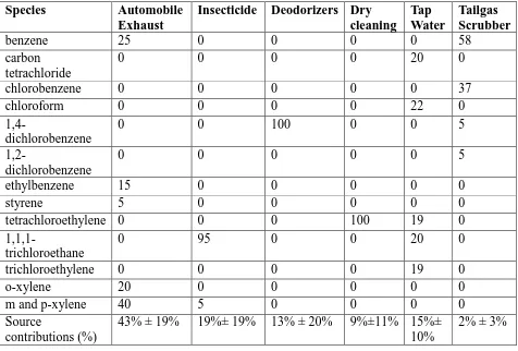
Table 2.23 Source profiles and source contributions (Anderson et al., 2002) ... 54

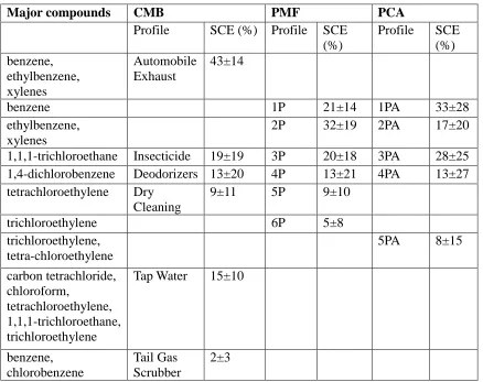
Table 2.24 Source profiles of different models and source contribution estimates (SCE) (Anderson et al., 2002)... 57

Table 2.25 Advantages and disadvantages of CMB, PMF, and PCA ... 59

Table 3.1 Sampling dates of winter and summer of year 2006 ... 62

Table 3.2 Sampler retrieval and retention rates in year 2005 and 2006 ... 63

Table 3.3 Percentage of sites with different number of samples obtained in each season and annual of 2005 and 2006 ... 64

Table 3.4 55 PAMS species and fitting species (marked with *) (Templer, 2007) .... 66

Table 3.5 Percentage of the species concentration below MDL ... 68

Table 3.6 Inputs and outputs for CMB ... 70

Table 3.7 PMF model inputs and outputs of year 2006 ... 73

Table 3.8 Inputs and Output of PCA ... 75

Table 3.9 The species classification of seven classes ... 77

Table 3.10 Procedures of comparison among sources of CMB, PMF, and PCA ... 91

Table 3.11 ArcGIS inputs ... 92

Table 4.1 The mean concentration of the species of all sampling sites in winter and summer of year 2005 and 2006 (*fitting species) ... 95

Table 4.2 The season and year concentration ratio (*fitting species) ... 97

Table 4.3 Number of performance measures out of range in winter 2006 out of 47 sites ... 100

Table 4.4 Number of performance measures out of range in summer 2006 out of 45 sites ... 101

Table 4.5 Source contribution estimates and percentage for year 2005 and 2006 ... 102

xii

both years ... 106

Table 4.7 Sum percentage of seven classes in each PMF factor for winter 2006 .... 128

Table 4.8 Sum percentage of 7 classes in each PMF factor for summer 2006 ... 133

Table 4.9 List of sources and source contributions in winter and summer 2006 from PMF... 137

Table 4.10 Sources and the species accounted for 6% or more in profiles in winter and summer 2006 (pink shade indicates the same species in the same profiles of winter and summer) ... 139

Table 4.11 Components and species with absolute loadings equal or greater than 0.26 or greater in any of the nine components ... 145

Table 4.12 Principal components of winter 2006 and loadings 0.26 or greater ... 149

Table 4.13 Principal components of summer 2006 and loadings 0.26 or greater .... 153

Table 4.14 Sources from PCA in winter and summer 2006 (Pink shade indicates the same species with high loadings in the same profiles of winter and summer) . 157

Table 4.15 Source comparison of CMB, PMF, and PCA in winter 2006 ... 162

xiii

LIST OF FIGURES

Figure 3.1 Sampling sites for 2005 and 2006 ... 62

Figure 3.2 Gasoline-related sources from PMF identification procedures ... 79

Figure 3.3 Sources other than gasoline-related sources from PMF interpretation procedures ... 80

Figure 3.4 PCA sources identification procedures ... 88

Figure 4.1 Source contribution spatial maps in winter 2005 ...110

Figure 4.2 Source contribution maps in summer 2005 ...114

Figure 4.3 Source contribution maps in winter 2006 ...119

1

CHAPTER 1 INTRODUCTION

1.1Background

Air pollution from transportation, industries, and other sources causes unbalance

of the atmosphere in terms of the chemical composition. Air pollutants are harmful to

living things (Environment Canada, 2013). Air pollutants are grouped into four categories.

They are: criteria air contaminants, persistent organic pollutants (POPs), heavy metals,

and toxic pollutants. There is overlap between toxics and the pollutants in the other three

categories. Criteria air contaminants include Sulphur Oxides (SOx), Nitrogen Oxides

(NOx), Particulate Matter (PM), Volatile Organic Compounds (VOCs), Carbon Monoxide

(CO), and Ammonia (NH3) (Environment Canada, 2013). Many air pollution problems

including smog and acid rains are caused by the presence or the interactions of the

criteria air contaminants.

VOCs are organic compounds that produce vapour at room temperature and

pressure (Environment Canada, 2013). VOCs come from both indoor and outdoor

sources. Indoor sources include the manufacture and use of everyday products and

materials. The outdoor sources include transportation, the oil and gas industry, the use of

paints and solvents, home firewood burning etc (Environment Canada, 2014). The

reactive VOCs are primary precursors to the formation of ground-level ozone and

particulate matter in the atmosphere. Ozone and PM are the main ingredients of the smog

that have serious effects on living things. The health effects of VOCs include eye, nose,

and throat irritation; headaches, coordination loss, nausea; damage to organs including

2

Windsor, Ontario is polluted by various ambient air pollution sources. There are

automobile industries including a Ford Engine Plant, and a Chrysler Assembly Plant.

Huron Church Road is the corridor connecting traffic from Windsor to the busiest trade

route in North America, the Ambassador Bridge. Transboundary pollution is another

major source because Windsor is located in the airshed of Detroit, MI, and Ohio.

Residents in Windsor may suffer the polluted air blowing from Detroit and Ohio. In order

to address the air quality related problem caused by transboundary pollution, Canada and

the USA unveiled an international agreement between Canada and United States known

as the Border Air Quality Strategy (BAQS) (Environment Canada, 2003).

The pollutants from the emitters include PM, NOx, and VOCs (Wheeler et al.,

2011). Studying the ambient VOCs helps to understand and address the air pollution in

Windsor. In order to control the VOCs levels, it is crucial to understand the emission

sources contributing to the ambient VOCs.

Receptor models are useful for understanding the major sources of VOCs.

Receptor models were developed to utilize the concentration measured at the receptor

sites to determine the contributions of potential sources (US EPA, 2011). The common

receptor models include Chemical Mass Balance (CMB) (US EPA, 2014a), Positive

Matrix Factorization (PMF) (US EPA, 2014a), Unmix (US EPA, 2014a), and Principal

Components Analysis (PCA) (Mathworks, 2014). The previous studies show that the

receptor models have been applied to source apportionment in many places. The

examples were application of PMF at Egbert, Ontario (Vlasenko et al., 2009); PMF in

rural sites of British Columbia (Jeong et al., 2008); PCA in urban areas of Dalian, China

3

Many studies conducted VOC source apportionment for multiple years. However,

few of them compared the source contribution in different seasons due to the lack of

measurement data or other reasons. Few studies applied three receptor models and

compared the sources of different models, perhaps due to the lack of source profiles in

the study region, lack of time, or other reasons. Learning the seasonal variation of the

source contribution helps to understand the contributions of major sources in different

seasons. Using different receptor models helps to identify the potential sources not

provided by other models.

Few researchers studied the variation of ambient VOCs levels and the source

contributions from different sources in different seasons of one year, and same season of

two different years. Few studies conducted VOCs source apportionment by using three

receptor models, and comparing their results.

VOC concentrations in both winter and summer in year 2005 and 2006 in

Windsor were obtained in a study called “Windsor, Ontario Exposure Assessment”

(WOEAS) (Wheeler et al., 2011). There were ten VOCs source profiles of Windsor

prepared by Templer (2007). The CMB results of 2005 were obtained by Templer (2007).

Therefore, these studies were prerequisites for carrying out VOCs source apportionment

by using different receptor models.

1.2 Objectives

The overall objective is to study the seasonal variation of the ambient VOCs

4

summer, respectively from 2005 to 2006 in Windsor, Ontario. By applying three receptor

models, additional sources with low contribution to the VOCs levels other than the ten

sources in Templer (2007) were expected to be found. The specific objectives are:

1) Compare the ambient VOC concentrations of the winter and summer in years

2005 and 2006, respectively, to see if there was seasonal trend; compare the annual

concentration of year 2005 and 2006 to see the annual trend from year 2005 to 2006.

2) Run the CMB model with the VOCs concentration data of winter and summer

2006 to find out the major VOCs contributors

3) Compare the source contribution results of winter and summer in 2006 with

that of 2005 from CMB model to see if the major sources in the same season were similar.

4) Use ArcGIS 10.1 software to compute the spatial source contribution

distribution maps for each of the ten sources to see the spatial trends of different sources

emissions.

5) Use the PMF model to analyze the potential sources of VOCs and the

corresponding contributions for both winter and summer 2006. Identify the factors from

the factor profiles based on the knowledge of source characteristics, literature reviews,

and the potential sources in Windsor. Compare the sources in winter and summer to see

the commonalities and differences.

6) Use the PCA model to analyze the potential sources of VOCs for both winter

and summer 2006; identify the sources based on knowledge of source characteristics,

5

and summer to see the commonalities and differences.

7) Compare the sources input to CMB with those identified by PMF, and PCA to

see the common sources and the additional sources from PMF or PCA over and above the

6

CHAPTER 2

LITERATURE REVIEW 2.1Volatile Organic Compounds

VOC are any organic compounds that can produce vapour under room

temperature and pressure (Environment Canada, 2013). A number of individual VOCs

including benzene and dichloromethane have been assessed to be toxic under the

Canadian Environmental Protection Act (1999) (Environment Canada, 2013). Some

highly toxic VOCs cause serious health problems including eye, nose, and throat

irritation; headaches, loss of coordination, nausea; damage to liver, kidney, central

nervous system, and even cancer. The level of the health effect depends on the extent of

the exposure to the VOCs (US EPA, 2013).

Many VOCs react with sources of oxygen molecules such as NOx and CO in the

atmosphere in the presence of sunlight, and from ground-level ozone. Ozone is a

constituent of photochemical smog. The outdoor VOC emissions are regulated by US

EPA (US EPA, 2013b) in United States, and Environment Canada in Canada

(Environment Canada, 2014).

The sources of VOCs include transportation, solvent use, industrial source,

commercial fuel, and biogenic emission from deciduous trees. In 2012, VOC emissions

in Canada reached 1768 kilotonnes (kt). The largest VOCs contributor was the oil and gas

industry, with 34% (606 kt) of national emissions. The use of paints and solvents

contributed 18% (323 kt) of national emissions, followed by the off-road vehicles,

7 2.2 Receptor Models

Receptor models help decision makers to control the VOC emissions. Different

models have different functions. CMB is used for evaluating the source contributions

when the potential sources profiles in an area are known. PMF and PCA are used for

providing source profiles and their corresponding contributions. Similar as PMF, Unmix

utilizes with the concentration put into the model to provide the profiles with the relative

contributions, and a time-series of contributions (US EPA, 2014). There is a non-negative

constraint for both source composition and contributions of Unmix, same as PMF. Unlike

PMF or PCA, Unmix provides source profiles for every sample, because Unmix assumes

that for each source, there are some samples contain very little or no contribution from

that source (Norris et al., 2007). This restricts Unmix from identifying the infrequent or

small sources (Kotchenruther and Wilson, 2003).

The fundamental of the receptor models is solving the mass balance equations as

equation (1):

=∑ F + (1)

where is the concentration of the element i measured in sample k; F is the mass

fraction of the element i in source j for CMB and PMF, and loading of element i in factor

j for PCA; is the contribution of the source j at sample k for CMB and PMF, and score

of source j at sample k for PCA; and is the residuals between model calculation and

8

output for PMF and PCA. and are outputs for all three models.

2.2.1 Chemical Mass Balance

CMB is applied to provide the source contribution of the sources when the source

profiles in an area are known. The inputs include measurements of species concentration

and source profile. Outputs include source contribution of each source. Source profiles

are expressed as fractional abundances of common property in different emissions. To get

the source profiles, the obtained samples from different emitters should be analyzed to

determine the properties. The properties are then normalized (scaled) to some common

property in the emissions from all sources by converting the measurements into ratio of

fractional abundances. The sum of the percentage of individual species in a profile should

be 100%. The species with high fractional abundance or the only measured species in the

source could be identified as species markers for the emission (Watson et al., 2004).

Preparation of the source profiles is time consuming and costly. A more common

method is to apply the available source profiles. However, users must be cautious when

choosing the source profiles. The potential sources and the source profiles compositions

for one place may not fit another. The source profiles should be a group of sources

instead of several single emission sources. The “Collinearity” happens when there are

two or more similar source profiles. Two or more CMB equations are redundant and the

equations cannot be solved. This could cause one source contribution high; while another

negative. In order to avoid this problem, similar source profiles should be grouped as one

9

property that CMB model can accept. CMB protocol recommends using the sum of the

55 Photochemical Assessment Monitoring Stations (PAMS) target hydrocarbons as the

common normalization standard for source profiles (Watson et al., 2004). The source

contribution output could be positive or negative values. The negative source

contributions could be replaced with zero in the post-processing.

CMB solves the equations on sample basis. It provides the source contribution

solutions for each sample as output.

There are six fundamental assumptions for CMB model as in CMB protocol

(Watson et al., 2004). They are:

1) The composition of the source profiles will not change in the process of

transportation between sources and receptors

2) There is no chemical reaction between the compounds

3) Every potential source to the pollution at receptor sites in the area is identified

and characterized.

4) Each identified source is independent with the others.

5) The number of the compounds is larger than that of the sources.

6) The uncertainties of the measurements are random, and with normal

distributions.

For assumptions 1 and 2, the chemical composition of compounds measured at

10

because CMB apportions the measured compounds to the sources following the given

proportion in the source profiles. CMB derives the best combination of the source

contribution at each site to explain the measurements and the source profiles. This could

be hardly achieved in reality because some reactive chemicals would react with others or

decay in the process of transportation. For assumption 3 and 4, CMB assumes that there

is no other source other than the provided source profiles in the area. Each source has

nothing to do with the others. As a matter of fact, there could be more sources

contributing to the receptors. The least squared solution requires random and uncorrelated

uncertainties of the measured concentrations. However, the accurate distribution of the

errors is hard to obtain.

The variance weighted least squared solution was applied to solve the mass

balance equations to find out the best solution of explaining the concentration

obtained at the receptor sites (Watson et al., 2004). The variance weighted least squared

solution is described in equation (2) (Watson et al., 2004):

∑

∑

!

" ₍₂₎

where # $_{% ∑}

$

&

where $ _{is one standard deviation of the measured concentration of compound i in}

sample k and $ _{is one standard deviation of the fraction of compounds i in source j.}

11

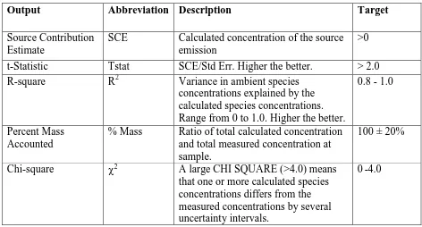
Source contribution estimate, t-statistics (Tstat), R-square, Percent Mass

Accounted (Mass %), and Chi-square are provided by the model to estimate model

performance. Table 2.1 shows the meaning and the target of each measure.

Table 2.1CMB Performance Measures (Watson et al., 2004)

Output Abbreviation Description Target

Source Contribution Estimate

SCE Calculated concentration of the source emission

>0

t-Statistic Tstat SCE/Std Err. Higher the better. > 2.0

R-square R2 Variance in ambient species

concentrations explained by the calculated species concentrations. Range from 0 to 1.0. Higher the better.

0.8 - 1.0

Percent Mass Accounted

% Mass Ratio of total calculated concentration and total measured concentration at sample.

100 ± 20%

Chi-square χ2 A large CHI SQUARE (>4.0) means

that one or more calculated species concentrations differs from the measured concentrations by several uncertainty intervals.

0-4.0

2.2.2 Positive Matrix Factorization

The fundamental of the PMF model is decomposing a matrix of speciated sample

data into two matrices—factor contributions and factor profiles. “Positive” refers to the

non-negative source composition and contribution output constraints. The factor profiles

12

in the study areas.

PMF model requires two input files including ambient concentrations and their

uncertainties. Two types of uncertainty files are accepted: sample-specific and

equation-based. The sample-specific uncertainty provides an estimate of the uncertainty for each

sample of each species. The dimension of the specific uncertainty is the same as the

concentration values. Another way to obtain concentration uncertainty is using equation

(3) (Vedantham and Norris, 2008):

Uncertainty='

( MDL, if concentration,method detection limit (MDL) (3)

Uncertainty=-uncertainty percent concentration%MDL

, if the concentration9MDL

PMF solves the mass balance equation (equation 1) by every species of each

sample, and provides one profiles, and the source contributions of each source in every

sample. The source contribution was given in the same order of factors. PMF operation

consists of three steps; they are base model run, bootstrap run, and the Fpeak run. The

follow up runs are based on the best run estimated in the previous one. Model is run

multiple times as specified, and the best run will be selected automatically based on the Q

(Robust) value of each run.

There are three kinds of outputs including Base model results, Bootstrap model

results, and the Fpeak model results. The base run results include factor profiles

13

factor contributions, and residuals of the calculated concentrations for each species of

samples.

The performance measures for PMF are shown in Base run outputs. The value of

Q (robust), Q (true), and whether each run is converged were shown in a table. The best

Goodness-of-fit run will be automatically marked with boldface in the Base Run report.

Details of each output are listed in Table 2.2.

Table 2.2 Performance measures of PMF

Name Description Target

Q(robust) Goodness-of-fit parameter calculated excluding outliers, defined as samples for which the scaled residual is greater than 4.

The lowest among all runs Q(true) Goodness-of-fit parameter calculated including all points,

defined as samples for which the scaled residual is greater than 4. Q(true) is greater than 1.5 times Q(robust) indicate that peak events may be disproportionately

influencing the model.

<=1.5 times Q(robust)

Convergence Whether the run converged or not Yes

Model outputs consist of factor profile tables, factor profile bar charts and pie

charts by compounds. Factor contribution files contain tables, scatter plots, and G-space

plots. The model performance was analyzed based on the residuals histogram charts, the

observed and predicted scatter tables and charts, diagnostics (e.g. Q Robust in table), and

14

Both scaled and before scaled residuals are provided in PMF model outputs.

Scaled residuals are between +3 and -3 on a histogram when they are normally

distributed. Any skewed or bimodal residuals indicate that the model calculated

concentration does not reproduce the observed concentrations well. The observed and

predicted scatter plots show the one on one line and the model calculated concentration

regression. The big bias between the predicted and the observed concentration also

indicate the model does not reproduce the measurement data well. Observed and

predicted time series is also on a line chart. The diagnostics table consists of the Q

(Robust), Q (True), converged or not (Yes/No), number of steps of run. Both Q (Robust)

and Q (True) indicate the goodness-of-fit parameter. Q (Robust) is calculated after

excluding the samples with scaled residuals greater than 4, whereas Q (True) is calculated

including all samples. The lowest Q (Robust) was highlighted to indicate the best

goodness-of-fit run. The large range of the Q (Robust) among all runs is the implication

of the poor stability between different runs. Aggregate contribution shows the boxplots of

annually contribution of each factor. G-space plot shows the scatter plots of factor versus

another factor. The desirable plot has all scatters distributing all over the space in between

X and Y axis, while the poor one always shows two clear edges, indicating that the two

factors are not independent with each other. Changing the number of factors could

eliminate this problem.

The poor performance of measurements is the implication of poor input dataset

reproduction. A second run is necessary. The model reproduction performance may be

improved by changing the characteristics of species with poor performance to “weak” or

15 2.2.3 Principal Component Analysis

PCA is used for proving the principal components that explain majority of the

variance of the input measurements. PCA only requires concentration measurements as

inputs. The outputs consist of coefficients containing loadings of each variable in every

measurement, eigenvalues for each component, variance explained in percentage by

descending order, and score. Each principal component is a linear combination of the

variables with loadings and scores (Joliffe, 2002). “Coefficients” profile consists of the

factor loadings.

Both loadings and scores have positive and negative values. Each component

represents a new dimension of the measurement data constructed in a dimension of

number of variables. Loadings represent the projection of the component vector on the

variable axis. When the measurements of variables are in the same units, the different

signs of the loadings of variables indicate the differences of the variables. The component

is interpreted as the factor that reveals the differences among the variables with different

signs. The higher the absolute loadings are, the greater the impacts the variables have on

determining the components. When the absolute loadings of the variables are close to

zero, the impact of the variables on the components is small. Similar to PMF, the

components should be interpreted by users based on the loadings of variables, the

knowledge of source characteristics, and the potential sources in the area.

The source contribution of each component to each species at a given sample is

calculated by multiplying the value of score of component at the given sample with the

16

given component to every species at a given sample derives the source contribution of the

component to the sample. The mean of the summations among all samples derives the

average source contribution of a given component. The measurement of samples is

reproduced by using the loadings and the scores profiles. Z score is applied when there

are not enough components with eigenvalue greater than one, or the input measurements

contain different units. Z score could be used to transform the original data by using the

standard deviation and the mean value of the variables in a dataset. There could be more

components with eigenvalues greater than one after applying Z score. However, Z score

is not recommended to be applied as some of the characteristics of the original data

would be lost. It is impossible to reproduce the measurements at samples when Z score is

applied. This is because reproduction of the measurements requires the raw scores of data;

however, Z score is a relative value, not an absolute value. For example, a low Z score of

a data does not mean a low raw score, instead, it suggests that the raw score is among the

lowest within that specific group (Gravetter and Wallnau, 2013).

Eigenvalues indicate the amount of the variance explained by each provided

component. Singular value decomposition (SVD) theorem is used to find out eigenvalues.

The components were ordered by eigenvalue of the factors, from high to low. Most

studies chose one as eigenvalue cut off.

The components could be rotated in order to reveal the relationship between

variables and components to the greatest extent without changing the relationship

between the components. The rotation methods consist of orthogonal rotation which

assumes that the given components are uncorrelated, and oblique rotation. The orthogonal

17

rotation assumes that the factors are correlated. The most widely used is varimax rotation

(Brown, 2009).

2.3VOC Source Characteristics

Source profiles are input for CMB and outputs for PMF and PCA. It is important

to understand the potential sources of Windsor, Ontario and their chemical compositions.

There were ten CMB sources profiles prepared by Templer (2007) for Windsor in year

2005. These source profiles could be applied if there is no major road or industries built

or out of operation compared with year 2005. The ten sources were Gasoline Exhaust,

Diesel Exhaust, Liquid Gasoline, Gasoline Vapour, Industrial Refinery, Architectural

Coatings, Commercial Natural Gas, Liquid Petroleum Gas, Coke Oven, and Biogenic

Emission. The source profiles consist of 55 non-methane hydrocarbons (NMHC) of

PAMS, and other species summed as one species group named as other. The full source

profiles are listed in Appendix A.

There are various compounds in different emission sources. Among the

compounds, some of them are the ground-level ozone precursors. Among those species,

55 NMHC are the target species of Photochemical Assessment Monitoring Sites (PAMS).

Most comprehensive VOC data derives from the PAMS. The sum of the 55 PAMS

species are recommended to be the common normalization standard for source profiles

18

Gasoline exhaust, diesel exhaust, liquid gasoline, gasoline vapour were all

vehicle-related sources. Gasoline and diesel are two types of fuel derived from crude oil.

The crude oil consists of up to 50% paraffins, 47% napthenes, and 3% aromatics

(Simanzhenkov and Idem, 2005). Gasoline is the product of distillation, cracking, and

treatment of crude oil refinery (Simanzhenkov and Idem, 2005). Finished gasoline

consists mostly of hydrocarbons and additives with approximately 150 separate

compounds. Additives are used to improve the performance and stability of the gasoline

(ATSDR, 2014). Energy is produced by burning hydrocarbons. The hydrocarbons in

gasoline are mostly with chain length between 4 to 12 carbon atoms (New Zealand

Ministry for the Environment, 2014). Table 2.3 shows the detailed chemical composition

19

Table 2.3 Gasoline Composition (weight %) (ATSDR, 2014)

n-alkanes % Branched alkanes

% cycloalkanes % olefin % aromatics %

C5 (e.g. n-pentane

3 C4 (e.g. iso-butane)

2.2 C6 (e.g. cyclohexane)

3 C6 (e.g. hexene)

1.8 Benzene 3.2

C6 (e.g. n-hexane)

11.6 C5 (e.g. iso-pentane

15.1 C7 (e.g. cyclo haptane

1.4 toluene 4.8

C7 (e.g. n-haptane

1.2 C6 (e.g. iso-hexane)

8 C8 (e.g. cyclo octane)

0.6 xylene

C9 (e.g. n-nonane)

0.7 C7 (e.g. iso-haptane)

1.9 ethylbenzene 1.4

C10-13 (e.g. n-decane, undecane, dodecane)

0.8 C8 (e.g. iso-octane)

1.8 C3-benzenes 4.2

C9 2.1 C4-benzenes 7.6

C10-13 1 others 2.7

Total 17.3 32 5 1.8 30.5

According to ATSDR (2014), branched alkanes and aromatics accounted for most

proportion of gasoline with 32% and 30.5%, respectively. Species n-alkanes also account

for significant amount with 17.3%. The anti-knock additives include oxygenates such as

ethers—methyl tertiary-butyl ether (MTBE), aromatic hydrocarbons and aromatic amines.

The aromatic hydrocarbons include toluene, xylene, and benzene. The aromatic amines

include m-toluidine, p-toluidine, p-tert-butylaniline, technical pseudocumidine,

n-methylaniline, and cumidines; and organometallic compounds (carbonyls) such as methyl

20

2014). The deflagration in the internal combustion engine could be adversely impacted

by autoignition, leading a phenomenon called “engine knock”. The anti-knock additives

provide high engine combustion ratio (octane rating) so that the gasoline combustion is at

high efficiency. Diesel contains mostly hydrocarbons with chain length between 8 to 17

carbon atoms including octane, decane, undecane, and nonane (New Zealand Ministry for

the Environment, 2014). Unlike gasoline engine, diesel engine does not rely on additives

because the hydrocarbons of diesel are heavier and more stable. Larger hydrocarbons can

be compressed to a high degree, creating high temperature that allows effective

combustion (Kraus, 2011).

Gasoline exhaust and diesel exhaust were products of fuel combustion. The

complete combustion of hydrocarbon results in carbon dioxide (CO2) and water (H2O);

incomplete combustion results in CO and hydrocarbons. Among the hydrocarbons in the

incomplete products, some of them are the evaporative unburned hydrocarbons; the

others are hydrocarbons transformed from the ones in gasoline into another forms.

Incomplete combustion could easily occur on hydrocarbons with higher amount of

carbon atoms when the oxygen supply is not enough. For example, same amount of

molecules of aromatics need more molecules of oxygen than isoalkanes do under the

same environment conditions. One molecule of benzene, toluene, and xylene require 7.5,

9, and 10 molecules of oxygen, respectively; whereas, one molecule of

isopentane/n-pentane requires only 6.5 molecules of oxygen. Thus, aromatics may not achieve

complete combustion as isoalkanes do when the same amount of oxygen supply is

provided. This happens particularly during the vehicle operation on idling or cold start.

21

Gasoline exhaust consists of 71% nitrogen, 14% CO2, 13% water, and 1-2% of CO,

hydrocarbon, and 0.1% NOx (ATSDR, 2014). Harley and Kean (2004) investigated the

chemical compositions of non-methane organic carbon (NMOC) emitted from motor

vehicles from 1991 and to 2001. Table 2.4 shows the percentage of the NMOC

percentage in gasoline exhaust profile.

Table 2.4 Composition of motor vehicles NMOC emissions (weight %) (Harley and Kean,

2004)

(a) Hydrocarbons in tunnel emissions (weight %)

Species 1991 1994 1995 1996 1997 1999 2001 Average

n-alkanes 9 9 9 9 9 9 9 9.0

isoalkanes 28 23 24 26 25 29 29 26.3

cycloalkanes 5 3 4 5 7 5 5 4.9

alkenes 18 18 17 18 17 15 17 17.1

aromatics 35 39 37 27 27 29 23 31.0

acetylene 4 5 5 4 5 5 9 5.3

oxygenates 0 0 0 7 6 3 3 2.7

carbonyls 0 3 3 5 4 5 5 3.6

22

(b) Aromatics hydrocarbons in tunnel emissions (weight %)

Species 1991 1994 1995 1996 1997 1999 2001 Average

benzene 6 6.5 6 4 4 5 4 5.1

toluene 8 10 10 9 8.5 10 9 9.2

m and p xylene 7 7.5 6 5 5.5 6.5 5 6.1

o-xylene 2 2.5 2 2 2 1 3 2.1

ethylbenzene 1 1.5 2 1 1 1 1 1.2

C9+ aromatics (1,2,4-trimethylbenzene, 1,3,5-trimethylbenzene,

1,2,3-trimethylbenzene)

13 11 11 6.5 7.5 8.5 7 9.2

According to Harley and Kean (2004), the composition of hydrocarbons in

gasoline exhaust consists mostly of aromatics (31.0%), followed by 26.3% iso-alkanes,

17.1% alkenes, and 9.0% n-alkanes. Thus, aromatics and iso-alkanes are expected to be

the dominant species with proportion of approximately 30% in gasoline exhaust. Toluene,

C9 aromatics, and xylenes are most abundant aromatics species in gasoline exhaust. The

percentage of aromatics is slightly higher than the isoalkanes are.

Diesel exhaust consists of 67% nitrogen, 12% CO2, 11% water, 10% oxygen, and

only 0.3% of Sulfur dioxide, particulate matter, hydrocarbon, and CO (Volkswagen,

2014), and 0.1% NOx,. Few detailed diesel exhaust VOCs composition is available. It

consists of 75% of saturated alkanes including n-alkanes, iso-alkanes, and cycloalkanes;

and 25% aromatics. The alkanes range from C10H20 to C15H28 (Diffen, 2014). Thus, there

are less aromatic in diesel than in gasoline exhaust (approximately 31.0%). Heavier

23

Liquid gasoline and gasoline vapour are two unburned vehicle emission. They

consist of the evaporative species from gasoline. Gasoline vapors are the releases of the

fuel vapour from the engine and the fuel system during vehicle operation. Liquid gasoline

is the migration of the fuel vapour from the evaporative canister, from leaks, and from

fuel permeation through joints, seals, and polymeric components of the fuel system

during the vehicle is resting (Harley and Kean, 2004). The resting losses process may due

to the diurnal temperature changes where the temperature rises during the day; hot soak

due to the high temperature after the engine is shut down for a short period (US EPA,

1994). In study of Harley and Kean (2004), composition of NMOC in liquid gasoline and

24

Table 2.5 Composition of NMOC in evaporative gasoline (weight %) (Harley and Kean, 2004)

(a) Composition of NMOC in Liquid Gasoline

Species 1995 1996 1999 2001 (Berkeley)

2001

(Sacramento)

Average

n-alkanes 9 6 7 9 9 8

isoalkanes 31 39 29 38 32 33.8

cycloalkanes 7 11 5 11 11 9

alkenes/dienes 9 2 15 2 5 6.6

aromatics 41 27 29 27 28 30.4

oxygenates 1 12 3 10 12 7.6

Others 2 3 5 3 3 3.2

(b) Composition of NMOC in headspace vapour (Harley and Kean, 2004)

Species 1995 1996 1999 2001 (Berkeley)

2001

(Sacramento)

Average

n-alkanes 23 16 20 20 20 19.8

isoalkanes 56 54 55 58 48 54.2

cycloalkanes 5 5 5 6 6 5.4

alkenes/dienes 11 5 2 6 5 5.8

aromatics 3 2 2 1 1 1.8

oxygenates 2 18 16 9 20 13

According to Harley and Kean (2004), the liquid gasoline samples were collected

at service stations. The components were identified by gas chromatography on a Hewlett

Packard Model 5890 II GC equipped with dual flame ionization detectors. The

components analysis was done by using DB-1 capillary column, with co-eluting peaks

resolved on a DB-5 column. The composition of headspace vapour was calculated by

25

the molecule fraction of different species in vapour phase is proportional with the

liquid-phase molecules fraction with coefficient of species vapour pressure. In other words,

given the same amount of molecules of species in liquid-phase, the higher the species

vapour pressure is, the more amounts of molecules the species present in vapour phase

(Harley and Kean, 2004).

The composition of the liquid gasoline is similar with gasoline with 33.8%

iso-alkanes, 30.4% aromatics, 9% cycloiso-alkanes, and 8% n-alkanes. Thus, isoalkanes and

aromatics are the main species in liquid gasoline. In headspace vapour, isoalkanes

accounted for over half of the total NMOC with 54.2%, followed by 19.8% n-alkanes.

Gasoline vapour consists mostly of isoalkanes. This is because the vapour pressure of

isopentane (77 kPa, 20°C) is much higher than that of the abundant aromatics in gasoline

including benzene (10.1kPa, 20°C), toluene (2.7 kPa, 20°C), and xylene (0.9 kPa, 20°C)

(CAMEO Chemicals, 2014). According to the vapor-liquid equilibrium theory for

non-ideal ethanol-gasoline mixtures, the amount of the molecules of isopentane is much larger

than that of the aromatics (Harley and Kean, 2004).

Petroleum refining is a series process of separation, conversion, and treatment.

The hydrocarbons are separated by fractionation in atmospheric and vacuum distillation

towers. Conversion is transforming the existing hydrocarbons into other forms of

hydrocarbons. The air pollutants emitted from refinery process includes particulate matter

(PM), metals, ammonia, CO2 (US EPA, 2011), sulphur dioxide, NO2, CO, hydrogen

26

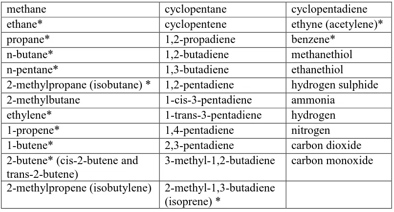
The “Proposed Risk Management Approach for Petroleum and Refinery Gases”

initiated by Health Canada and Health Canada compiled the main composition of

petroleum and refinery gases. The results are listed in Table 2.6.

Table 2.6 Major components of the petroleum and refinery gases (Government of Canada, 2013)

*55 PAMS species

methane cyclopentane cyclopentadiene

ethane* cyclopentene ethyne (acetylene)*

propane* 1,2-propadiene benzene*

n-butane* 1,2-butadiene methanethiol

n-pentane* 1,3-butadiene ethanethiol

2-methylpropane (isobutane) * 1,2-pentadiene hydrogen sulphide

2-methylbutane 1-cis-3-pentadiene ammonia

ethylene* 1-trans-3-pentadiene hydrogen

1-propene* 1,4-pentadiene nitrogen

1-butene* 2,3-pentadiene carbon dioxide

2-butene* (cis-2-butene and trans-2-butene)

3-methyl-1,2-butadiene carbon monoxide

2-methylpropene (isobutylene) 2-methyl-1,3-butadiene

(isoprene) *

The major gases of petroleum refinery emission are shown in Table 2.6. The

PAMS species emitted from petroleum refinery are ethane, propane, n&iso-butane,

n-pentane, ethylene, 1-propene, 1-butene, cis-2-butene and trans-2-butene, iso-butene,

27

Coal is processed to become coke (pure carbon) at the coke oven batteries (US

EPA, 2013). Coke oven emissions are a mixture of coal tar, coal tar pitch, volatiles,

creosote, PAHs including benzo(a)pyrene, benzanthracene, chrysene, and phenanthrene;

and metals. Coal tar volatiles include benzene, toluene, and xylenes(US EPA, 2013).

Coke Oven gas contains hydrogen, methane, ethane, CO, CO2, ethylene, propylene,

butylene, acetylene, hydrogen sulfide, ammonia, oxygen, and nitrogen (U.S. Government,

2011).

According to (Totten et al., 2003), liquid petroleum gas refers to the mixture of

ethane, propane, and butane that can exist under modest pressure at ambient temperature.

The butane/propane mixture is commonly used as fuel (Totten et al., 2003). Propane

accounted for at least 90% in the liquid petroleum gas (U.S. department of Energy, 2013).

This is because liquid petroleum gas tank is always under pressure at normal operating

temperature above the boiling point of -42 °C, and propane can be used from -40 °C to 45

°C; while and butane from 0 °C to about 110 °C. Thus, propane is more robust and

reliable compared to butane.

Commercial natural gas consists mostly of methane (95%), followed by ethane

(2.5%), propane (0.2%), n&iso-butane (0.06%), pentanes (0.02%), nitrogen (1.6%), CO2

(0.7%), hydrogen sulphide (trace), water (trace) (Enbridge, 2014). Ethane, propane are

the major NMHC in the Commercial natural gas.

Adhesives, painting and surface coatings are mixture of solids suspended in

solvent or diluent (water). The solvents mainly consist of VOCs (Lambourne and Strivens,

28

composition of the adhesives, painting and surface coatings depends on the solids, the

substrate on which it is going to attach, and the conditions of the use (Lambourne and

Strivens, 1999).

Architectural and industrial are two main uses of coatings. The solvents in

architectural coatings contain mostly VOCs including toluene, styrene, and xylene

(Lambourne and Strivens, 1999). Architectural coatings are applied under ambient

temperature where the paint dries by atmospheric oxidation or the evaporation. The small

polymer particles are expected to form as dispersion in water or an organic solvent so that

a solid coating could be attached on the surface. This occurs when the temperature is

above the polymer's glass transition temperature. However, adding the solvents

containing VOCs could lower this property when the temperature is below the transition

point. Industrial coatings include automotive paints; can coatings, coil coatings, furniture

finishings and road-marking paints (IHS GlobalSpec, 2014). Many industrial finishing

processes are under heat. The ‘thermosetting’ polymers mixed with alkyd combined with

amino resin were often used in industrial coating processes. However, the composition of

the industrial coatings is more diverse in terms of the requirements and factory conditions

(Lambourne and Strivens, 1999).

Adhesives consist of sticky solids that make pieces of material stick together. One

of the polymer-solvent systems is polychloroprene distributed in solvents mixed with a

ketone or an ester, an aromatic and aliphatic hydrocarbon. The aliphatic hydrocarbon

could be selected from naphtha, hexane, heptane, acetone, methyl ethyl ketone, benzene,

xylene, and toluene (Wypych, 2000). Among the composition of solvent in the

29

toluene are VOCs.

Biogenic emissions are released from trees and shrubs. They consist of isoprene

and monoterpenes such as α-pinene and β-pinene (Lewandowski et al., 2013). The

species are commonly found in mid-latitude regions including Canada (Bonn et al., 2004).

The concentration of isoprene is higher in summer as there is much more leaves on the

deciduous trees.

2.4 VOCs Source Apportionment Studies

2.4.1 CMB Studies

CMB has been applied to VOC source apportionment in places all over the world.

30

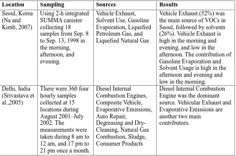
Table 2.7 CMB VOCs source apportionment application

Location Sampling Sources Results

Seoul, Korea (Na and Kimb, 2007)

Using 2-h integrated SUMMA canister collecting 18

samples from Sep. 8 to Sep. 13, 1998 in the morning, afternoon, and evening.

Vehicle Exhaust, Solvent Use, Gasoline Evaporation, Liquefied Petroleum Gas, and Liquefied Natural Gas

Vehicle Exhaust (52%) was the main source of VOCs in Seoul, followed by solvents (26%). Vehicle Exhaust is high in the morning and evening, and low in the afternoon. The contribution of Gasoline Evaporation and Solvent Usage is high in the afternoon and evening and low in the morning. Delhi, India

(Srivastava et al.,2005)

There were 360 four hourly samples collected at 15 locations during August 2001–July 2002. The

measurements were taken during 8 am to 12 am, and 17 pm to 21 pm once a month.

Diesel Internal Combustion Engines, Composite Vehicle, Evaporative Emissions, Auto Repair,

Degreasing and Dry-Cleaning, Natural Gas Combustion, Sludge, Consumer Products

Diesel Internal Combustion Engine was the dominant source. Vehicular Exhaust and Evaporative Emissions are another two main

31

Table 2.7 – continued 1

Helsinki and Ja¨rvenpa¨a¨, Finland (Helleän et al., 2006) Using evacuated stainless steel canisters (6 L). The 24-hour

concentration measurements were conducted in Helsinki in

February, May, and September of 2004 on 16 different days and in Ja¨rvenpa¨a¨ in November and December of 2004 and in January of 2005 on 10 different days. Traffic-Related, Wood Combustion, Commercial Natural Gas, Biogenic Hydrocarbon, Dry-Cleaning

Major source in urban site were traffic. At the residential site, Liquid Gasoline, and Wood Combustion made higher contributions than traffic sources. Biogenic compounds such as isoprene, also has significant

anthropogenic sources such as Wood Combustion. Those compounds sometimes can be mistaken for traffic-related compounds (e.g.,

Benzene).

Urban area of Dunkerque, French (Badol et al., 2008)

Hourly data of 53 VOCs measured continuously during 1 year. There were 7000 samples collected.

Urban

Sources: Urban Heating, Solvent Use, Natural Gas Leakage, Biogenic Emissions, Gasoline

Evaporation and Vehicle Exhaust seven industrial sources: Hydrocarbon Cracking, Oil Refinery, Hydrocarbon Storage, Lubricant Storage, Lubricant Refinery, Surface Treatment and Metallurgy.

Vehicle Exhaust contribution in urban was 40%-55%. In industrial area, it was around 60% and could reach 80%. The Vehicle Exhaust

contribution varies from 55% in winter down to 30% in summer. Metropolitan area of Saitama in Tokyo, Japan (Morino et al., 2011) Hourly

concentration of C2 -C8 non methane hydrocarbons (NMHCs) were measured throughout year of 2007. More than 6000 data were obtained. Gasoline Vapour, Petroleum Refinery, Light-Duty Gasoline, Super-Light-Duty Gasoline, Diesel Vehicle, Liquefied Natural Gas, Liquefied Petroleum Gas, and Paint Solvent

32

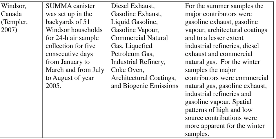
Table 2.7 - continued 2

Windsor, Canada (Templer, 2007)

SUMMA canister was set up in the backyards of 51 Windsor households for 24-h air sample collection for five consecutive days from January to March and from July to August of year 2005. Diesel Exhaust, Gasoline Exhaust, Liquid Gasoline, Gasoline Vapour, Commercial Natural Gas, Liquefied Petroleum Gas, Industrial Refinery, Coke Oven, Architectural Coatings, and Biogenic Emissions

For the summer samples the major contributors were gasoline exhaust, gasoline vapour, architectural coatings and to a lesser extent

industrial refineries, diesel exhaust and commercial natural gas. For the winter samples the major

contributors were commercial natural gas, gasoline exhaust, industrial refineries and gasoline vapour. Spatial patterns of high and low source contributions were more apparent for the winter samples.

According to the six papers, CMB was applied for investigating the ambient

VOCs in Europe, North America, and Asia. The data collection period ranged from a

week to one year; and the number of samples collected ranged from 16 to thousands.

Among the sources in the review, Diesel Exhaust, Gasoline Exhaust, Liquid Gasoline,

Gasoline Vapour, Coke Oven, Architectural Coatings, Biogenic Emissions, Liquefied

Petroleum Gas, and Industry Refinery were the sources included in this paper. The other

sources were Liquefied Natural Gas, Auto Repair, Degreasing and Dry-Cleaning, Wood

Combustion, Sludge, Consumer Products, Hydrocarbon Cracking, Hydrocarbon Storage,

Lubricant Storage, Surface Treatment and Metallurgy, and Lubricant Refinery. The

review showed that vehicle-related sources were the major VOC contributors in all VOCs

source apportionment studies listed in Table 2.7. The VOC contributions from sources

33

Kimb, 2007), Badol et al. (2008), and Templer (2007).

2.4.2 PMF Studies

There were 17 papers found involving the VOCs source apportionment by using

PMF model, among them, nine papers included the source profiles from PMF. They are

Wang et al. (2013), Cai et al. (2010), Wei et al. (2014), Song et al. (2008), Morino et al.

(2011), Sauvage et al. (2009), Lam et al. (2013), Yuan et al. (2009), Song et al. (2007),

and Chan et al. (2011). Out of the source profiles in nine papers, there were three

Gasoline Exhaust profiles, two Liquid Gasoline profiles, three Diesel Exhaust profiles,

three Gasoline Vapour profiles, eight paint and Solvent profiles, seven Liquid Petroleum

Gas profiles, six Petrochemical sources profiles, and one Commercial Natural Gas profile.

Coke Oven was not observed in any of the nine papers. The source profiles prepared in

Templer (2007) were also included. The additional species other than the 55 PAMS

species of CMB model were put at the end of each profile. The source profiles in

concentration units were converted into percentage. The percentage of the species in each

profiles were ranked in descending order. Table 2.8 shows any species with percentage of

6% or more in order to reveal the potential species markers in different profiles. The

34

Table 2.8 Gasoline Exhaust profiles from PMF in previous studies

(a) Previous studies 1

Song et al. (2008) Yuan et al. (2009) (location 1)

Yuan et al. (2009) (Location 2)

Templer (2007)

species Per cent (%)

species Per

cent (%)

species Per

cent (%)

species Per cent (%)

acetylene 16.8 toluene 18.3 benzene 30.5 other 24.6

propane 12 isopentane 15.2 toluene 27.3 toluene 7.7

isopentane 11.9 benzene 9.1 isopentane 10.5 isopentane 6.9

ethane 11.7 pentane 8.7 2-methylhexane 7.7 ethylene 6.5

ethylene 9.9 hexane 7.7 pentane 4.1 m and

p-xylene

4.1

butane 8.4 2-methylpentane 5.6 butane 4 acetylene 3.7

toluene 6.6 3-methylpentane 4.7 3-methylpentane 3.2 2,2,4-trimethylpe ntane

3.5

isobutane 6.2 3-methylhexane 4.1 hexane 3 benzene 3.3

(b) Previous studies 2

Gasoline Exhaust (Wang et al., 2013) Car 1 Species Mass

per cent (%)

Car 2 Species Mass per cent (%)

Car 3 Species Mass

per cent (%)

Average

ethylene 12.8 ethylene 11.4 ethylene 11.2 11.8

toluene 11.1 toluene 10.6 toluene 12.1 11.3

benzene 9.1 benzene 9.4 benzene 8.0 8.8

isopentane 6.7 isopentane 7.4 isopentane 5.8 6.6

propylene 5.4 alkyne ethyne 6.3 1,3-dimethylbenzene 5.4

According to the Gasoline Exhaust profiles in Table 2.8, species including

isopentane, toluene, and benzene are the common species markers (Song et al., 2008;

Yuan et al., 2009; Templer, 2007; Wang et al., 2013). Species such as acetylene (Song et

35

2013), are another two species markers. Toluene and benzene were expected to be the

species markers according to the vehicle emission study of Harley and Kean (2004).

Ethylene is another significant species marker for gasoline exhaust. There were three

Liquid Gasoline profile literature reviews. They are listed in Table 2.9.

Table 2.9 Liquid Gasoline profiles from PMF in previous studies

Liquid/evaporated/exhaust gasoline (Song et al., 2008)

Evaporated and Liquid Gasoline (Yuan et al., 2009)

Liquid Gasoline (Templer, 2007)

Species Per cent

(%)

Species Per cent (%)

Species Per cent

(%)

isopentane 21.8 butane 21.1 toluene 14.9

acetylene 18.5 isopentane 19.5 m and p-xylene 9.8

ethylene 11.6 isobutane 14.6 isopentane 9.4

pentane 6.3 propane 8.7 pentane 6.3

toluene 5.8 benzene 8.1 other 4.6

MTBE 4.6 pentane 7.2 2-methylpentane 4.3

According to the Liquid Gasoline profiles in Table 2.9, species n&isopentane

(28.1%, 26.7%, and 15.7%) is the common species marker for Liquid Gasoline (Song et

al., 2008; Yuan et al., 2009; Templer, 2007). Toluene (5.8%, 4.5%) is another species

marker according to Song et al. (2008) and Templer (2007). The large proportion of

isopentane and toluene agree with the study of Harley and Kean (2004). In Harley and

Kean (2004), the isoalkanes and aromatics are two dominant species classes with

isoalkanes percentage slightly outweighing aromatics. There were five Diesel Exhaust

36

Table 2.10 Diesel Exhaust profiles from PMF in previous studies

(a) Previous studies 1

Lam et al. (2013) Yuan et al. (2009) (Location 1) Yuan et al. (2009) Location 2

Species Per

cent (%)

Species Per cent

(%)

Species Per cent (%)

toluene 19 toluene 11.9 isopentane 17.1

butane 15.6 isopentane 9.9 isobutane 15.7

hexane 11.5 m and p-xylene 7.8 propane 14.9

propane 10.9 benzene 7.1 pentane 10.1

acetylene 9.2

1,2,4-trimethylbenzene

6 toluene 9.6

isobutane 6.9 decane 5.9 1-butene 8.6

ethylbenzene 6.4 propane 5.2 butane 7.9

ethylene 5.6 hexane 5.2 iso-butene 6.8

(a) Previous studies 2

Song, et al. (2007) Templer (2007) Species Per cent

(%)

Species Per cent

(%)

ethane 0.2 m and p-xylene 10

acetylene 0.2 other 9.2

ethylene 0.1 ethylene 8.9

decane 0.1

1,2,4-trimethylbenzene 6.8

isopentane 0.1 undecane 4.8

benzene 0 toluene 4.1

propane 0 3-ethyltoluene 3.8

toluene 0 propylene 3.6

According to the Diesel Exhaust profiles in Table 2.10, the species including

decane (5.9%, 10%) (Yuan et al., 2009; Song, et al., 2007) and undecane (4.8%) (Templer,