Improving productivity through line balancing : a case study

Jumal Mekanikal

Disember 2002, Bil. 14, 48 - 62

IMPROVING PRODUCTIVITY THROUGH LINE

BALANCING - A CASE STUDY

Lim Chuan Pei Masine Md. Tap

Faculty of Mechanical Engineering, Universiti Teknologi Malaysia,

81310 UTM Skudai

ABSTRACT

This paper describes a case study conducted at a manufacturing company aimed at improving productivity using line balancing. Two altematives were generated using different assignment rules. However selection of the most suitable altematives cannot be made based on line balancing alone as they appear similar based on line balance loss. Thus the robustness of the altematives were tested and evaluated using a 16factorial ANOVA. Selection of the most suitable solution is then made based on these results.

Keyword: Productivity improvement, Line balancing, Simulation.

1.0 INTRODUCTION

Many researchers have reported various productivity techniques and performance measures designed to monitor and improve system performance in an organization [1,2,3,4]. Some deal with specific problems such as inventory, scrap and set-up time reduction, with the aim of increasing manufacturing productivity. One of these techniques is line balancing.

Line balancing aims to match the output rate to the production plan [5]. This will assist management in ensuring on-time delivery and prevents buildup of unwanted inventory. Johnson [6] expresses the problem of line balancing as 'a set of nondivisible tasks to be performed, Each task has a known deterministic performance time. A partial ordering of tasks by precedence constraints is specified. The problem is to assign these tasks to assembly stations, so that the necessary number of station is minimized.' The steps to line balancing has been detailed out by Hoffman [7].

simulation and 16-factorial ANOVA. Based on these results the appropriate altemati ve is recommended.

2.0 PROBLEM DEFINITION

Currently, the SL-D assembly line faces the problem of fulfilling the targeted production plan. To fulfill the production plan, overtime work is conducted. This increases the production costs and reduces company profit.

Figure 1 shows the comparison between the actual output and the production target for the month of July. It is representative of other months. This output is based on normal working period of one shift per day without overtime. The line across the graph is the targeted output of the product which is 850 units per day. This production capacity is calculated by the production planner based on the available machines and human resources. It shows that only a few of the daily actual outputs reached the targeted production capacity. Although 20% of the time output surpassed the targeted production, it cannot compensate for the other 80%. Observations and investigations show that the main cause for this is due to unbalanced assembly line. Figure 2 shows graphically the line balance loss (LBL) of each work station. It also shows that some workstations tend to be the cause for bottlenecks as these stations handled more workload as compared to other stations, for example workstations 3, 5, 14 and 39. In contrast, workstations 35 and 38 are very often idle.

The LBL percentage is presented to identify the seriousness of the problem. LBL is calculated as follows:

Line Balance Loss Percentage:

nT -

Lt.

%LBL

=

nT_max

= (39X35.84)-519.46 XlOO% (39X35.84)

=

where;

n

=

=

Jurnal Mekanikal,Disember2002

The result shows that this assembly line is more than 60% unbalanced. Thus, some effective action must be taken to balance the assembly line, as well as to increase the productivity of the assembly line.

To facilitate line balancing, other information related to the line such as precedence relationship of the work tasks or workstation was also collected. Precedence requirements are physical restrictions on the order in which operations are performed on the assembly line. Figure 3 illustrates the precedence diagram for the assembly line SL-D. It portrays the elemental tasks to be performed and sequence requirements of the assembly processes.

3.0 PROPOSED SOLUTION

The assembly process involves a set of workstations, each carrying out a specific task or tasks in a restricted sequence. It is important that tasks be allocated to each workstation as evenly as possible to avoid bottlenecks and excessive idle time. Line balancing involves assigning and balancing tasks between workstations of the assembly line in order to minimise balance delay, labour force and ultimately minimising the total production cost. Two alternative solutions are proposed. Ranked positional weight was used to generate Alternative 1. Whereas, Alternative 2 is generated by modifying Alternative 1 based on the concept of eliminating, combining, simplifying the assembly process without any additional machine and manpower in the hope that further improvement may be achieved.

The cycle time of each workstation is kept to within 29 seconds. This value is calculated based on the required production rate and the cycle time.

3.1 Alternative 1

The alternative solution is generated based on the 'ranked positional weight' rule in selecting tasks for workstations. Specifically, this rule states that tasks that meet precedence criteria are assigned according to their positional weights, which are times for a given task plus the task times of all those that follow. The task with the highest positional weight would be assigned to the first station. Recommended changes to the assignment of task to each operator in the line are: • Transfer work task of operator 3 to operator 2 (back board sub-assembly).

Thus saving one manpower in the line.

• Combined work task of operators 4, 5 and 6 in baffle board sub-assembly to meet total process time of 25 seconds. In this case, using multiskilled operator to operate the workstation as a team rather than as independent workers.

• Transfer work task of operator 12 to operator 11 (triangle wood attachment) and adjacent operator 10 to assist operator 11. Thus, saving one manpower in the line.

• Combined work tasks of operator 14 (sanding and touching up) with operator 13 to eliminate the slack time between workstations 7 and 8.

• Combine work task of operator 31 (duct fixing) and operator 30, and using multiskilled operator to operate the workstation as a team rather than as independent workers.

• Transfer work task of operator 44 (polyfoam placement) to operator 43. Thus, saving one manpower in the line.

3.2 Alternative 2

The second alternative solution is generated by modifying the Alternative 1.

Modification is made based on the concept of eliminating, combining and simplifying the assembly process without any additional machine and manpower. Changes to the assignment of work task to each operator in the line are:

• Transfer work task of quality operator QA2 (electronic component checking) to QAl (terminal cord plug in), to eliminate QA2 in the line.

• Transfer work task of operator 24 (wood ADH) to operator 23 (layer protection).

• Transfer work task of operator 26 (lens screwing) to operator 25 (lens fixing), and operator 25 would take over the entire combined work tasks.

• Eliminate operator 29 (screwing), and operator 28 (front panel fixing) would take over the combined work tasks. Improve work method of operators 27 and 28 (station 13) to deal with cycle time in 29 seconds by reducing the task time. • Combine workstation 28 (QC appearance checking) and workstation 27 (set

cleaning and matching). In this case, using two multiskilled operators to operate the workstation as a team rather than as independent workers. Thus, saving two manpower in the line.

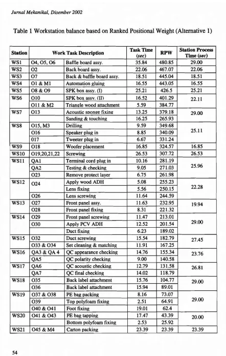
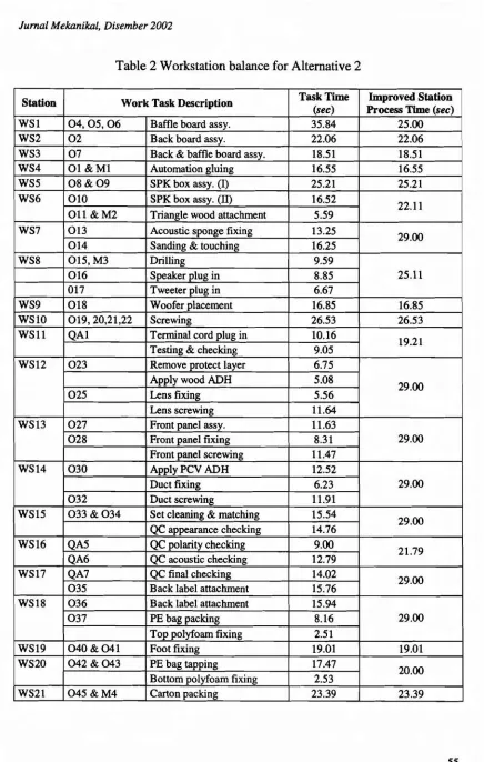
Tables 1 and 2 show the workstations and process time of each station in SL-D assembly line for Alternatives 1 and 2 respectively.

Informulating Alternatives 1 and 2, these assumptions have been made; i. The process cycle time for every work task is based on existing records. ii. Mean time between failure and mean time to repair is modelled using the

exponential distribution [8].

iii. For the combined work tasks, the new process cycle time is the average of total time of the work tasks.

iv. For the task that is assigned to another operator, the cycle time is based on records of the existing system.

v. The machine speed or production rate is constant.

vi. The skill and experience level of all operators are considered to be the same.

Jumal Mekanikal, Disember2002

4.0 EVALUATION OF PROPOSED SOLUTIONS

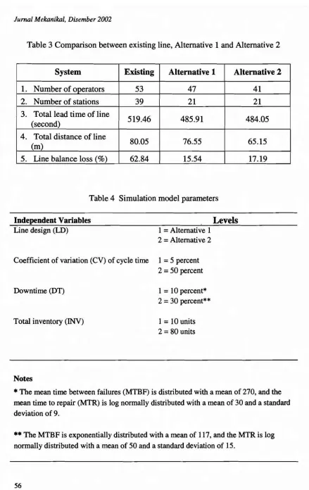
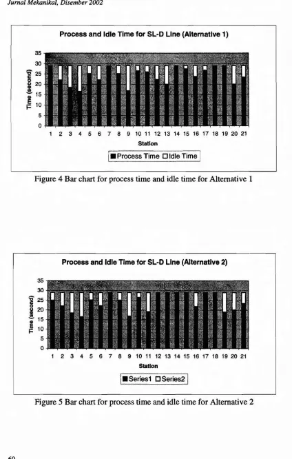
Figures 4 and 5 show the bar charts for process time and idle time for Alternatives I and 2 respectively based on Tables I and 2 respectively. Table 3 summarises the differences in the results of various parameters of the existing and alternative systems. These parameters include line balance loss, number of operator, number of station, total lead-time of line and total distance of line. It

shows that Alternatives 1 and 2 have the potential of producing significant improvement over the existing situation.

However comparison between Alternatives I and 2 shows that overall Alternative 2 is slightly better. Alternative 2 requires less operator as compared to Alternative I while all other parameters are almost equal. To further verify that Alternative 2 is indeed the best alternative the robustness of both alternatives is tested.

Simulations have been carried out to test the robustness of these alternatives. Witness software was used for this purpose. The model of each alternative is subjected to extreme levels of station downtime, processing time and inventory as shown in Table 4. This simulation uses a 2 x 2 x 2 x 2 (16) factorial ANOVA along with pair-wise comparisons and family confidence intervals to study the following;

1. The effect of high and low levels of station coefficient of variation to the performance of each line.

n. The effect of high and low levels of station downtime to the performance of each line.

iii. The effect of high and low levels of inventory in the system to the performance of each line.

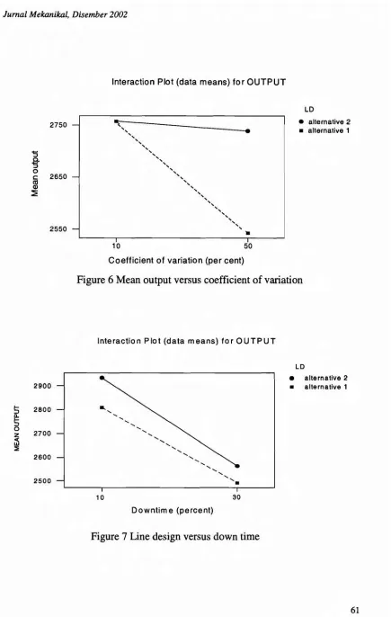
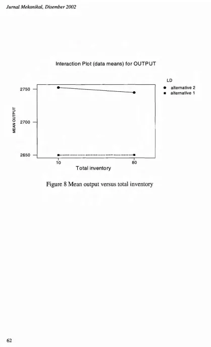
Figures 6, 7 and 8 show the results of the simulation experimentations. Performance is measured based on the total output of each line. These results indicate that Alternative 2 is less affected by variability within the system than Alternative 1. Alternative 2 appears to be able to achieve higher output level under both levels of system down time, coefficient of variation and extreme levels of inventory. Assembly lines less affected by variability within the system should enable management of factory to provide more reliable delivery of product. Thus, Alternative 2 is selected as the best alternative as it not only uses the least number of operators, it is also robust and less sensitive to changes.

5.0 CONCLUSION

outperformed the existing system. However, it was difficult to choose the best alternative as they were almost equal to each other. Thus the robustness of each alternative were simulated and evaluated using a 16-factorial ANOVA. Alternative 2 was found to be more robust than Alternative 1 and it is proposed to the management of the company.

This study also shows that in line balancing problem, line balancing loss may not be the only criterion or measurement that may be used to determine the optimum alternative especially in cases where alternatives are almost equal to each other. The robustness of these solutions against the varyingly important parameters should also be considered. A robust system will be able to perform better in a real life environment where change and uncertainty are common.

ACKNOWLEDGEMENT

The authors acknowledge the support given by Universiti Teknologi Malaysia in conducting this project.

REFERENCES

1. Baines, A., 1997, "Productivity measurement and reporting", Work Study 46(5), PP. 160-161.

2. Jonsson, P. and Lesshammar, M., 1999, "Evaluation and improvement of manufacturing performance measurement systems - the role of OEE', International Journal of Operations and Production Management 19(1), PP. 55-78.

3. Daniels, S., 1997,"Back to basics with productivity techniques", Work Study 46(2), PP. 52-57

4. Craig, C.E. and Harris, R.C., 1973,"Total Productivity Measurement At The Firm Level", Sloan Management Review, PP. 13-28.

5. Krajewski, LJ. and Ritzman L.P., 1998,"Operations Management: Strategy and Analysis", Addison-Wesley.

6. Johnson, R.V" 1983, "A Branch And Bound Algorithm For Assembly Line Balancing Problems With Formulation Irregularities", Management Science, PP. 1309-1324.

7. Hoffmann, T.R., 1990, "Assembly Line Balancing: A Set Of Challenging Problems", International Journal of Production Research, Vol. 28, PP. 1807-15.

Jumal Mekanikal, Disember 2002

Table 1 Workstation balance based on Ranked Positional Weight (Alternative 1)

Station Work Task Description Task Time RPW Station Process

(sec) Time(sec)

WSI 04,05,06 Baffle board assy. 35.84 480.85 29.00

WS2 02 Back board assy. 22.06 467.07 22.06

WS3 07 Back & baffle board assy. 18.51 445.04 18.51

WS4 01&Ml Automation gluing 16.55 443.05 16.55

WS5 08&09 SPK box assy.(1) 25.21 426.5 25.21

WS6 010 SPK box assv.(ll) 16.52 401.29 _22.11

011 &M2 Trianzle wood attachment 5.59 384.77

WS7 013 Acoustic snonae fixinz 13.25 379.18 _29.00

Sanding & touching 16.25 265.93

WS8 015, M3 Drilling 9.59 349.68

016 Speaker plug in 8.85 340.09 25.11

017 Tweeter plug in 6.67 331.24

WS9 018 Woofer placement 16.85 324.57 16.85

WSlO 019,20,21,22 Screwing 26.53 307.72 26.53

WSll QAl Terminal cord plug in 10.16 281.19

QA2 Testing & checking 9.05 271.03 25.96

023 Remove protect layer 6.75 261.98

WS12 ₀₂₄ Apply wood ADH 5.08 255.23

Lens fixing 5.56 250.15 22.28

026 Lens screwing 11.64 244.59

WS13 027 Front panel assy. 11.63 232.95 _19.94

028 Front panel fixing 8.31 221.32

WS14 029 Front panel screwing 11.47 213.01

030 Apply PCV ADH 12.52 201.54 29.00

Duct fixing 6.23 189.02

WS15 032 Duct screwing 15.54 182.79 _27.45

033 &034 Set cleaning & matching 11.91 167.25

WS16 QA3 &QA4 QC appearance checking 14.76 155.34 _23.76

QAS QC polarity checking 9.00 140.58

WS17 QA6 QC acoustic checking 12.79 131.58 _26.81

QA7 QC final checking 14.02 118.79

WS18 035 Back label attachment 15.76 104.77 _29.00

036 Back label attachment 15.94 89.01

WS19 037 & 038 PE bag packing 8.16 73.07

039 Top polyfoam fixing 2.51 64.91 29.00

040&041 Foot fixing 19.01 62.4

WS20 041 &043 PE bag tapping 17.47 43.39 _20.00

Bottom polyfoam fixing 2.53 25.92

Table 2 Workstation balance for Alternative 2

Station Work Task Description Task Time Improved Station (sec) Process Time(sec)

WSI 04,05,06 Baffle board assy. 35.84 25.00

WS2 02 Back board assy. 22.06 22.06

WS3 07 Back & baffle board assy. 18.51 18.51

WS4 01 &Ml Automation gluing 16.55 16.55

WS5 08&09 SPK box assy.(I) 25.21 25.21

WS6 010 SPK box assy. (II) 16.52

22.11 011 &M2 Triangle wood attachment 5.59

WS7 013 Acoustic sponge fixing 13.25

29.00

014 Sanding & touching 16.25

WS8 015, M3 Drilling 9.59

016 Speaker plug in 8.85 25.11

017 Tweeter plug in 6.67

WS9 018 Woofer placement 16.85 16.85

WSIO 019,20,21,22 Screwing 26.53 26.53

WSll QAl Terminal cord plug in 10.16

19.21 Testing & checking 9.05

WS12 023 Remove protect layer 6.75

Apply woodADH 5.08

29.00

025 Lens fixing 5.56

Lens screwing 11.64

WS13 027 Front panel assy. 11.63

028 Front panel fixing 8.31 29.00

Front panel screwing 11.47

WS14 030 Apply PCVADH 12.52

Duct fixing 6.23 29.00

032 Duct screwing 11.91

WS15 033 &034 Set cleaning & matching 15.54

29.00 QC appearance checking 14.76

WS16 QA5 QC polarity checking 9.00

21.79

QA6 QC acoustic checking 12.79

WS17 QA7 QC final checking 14.02

29.00

035 Back label attachment 15.76

WS18 036 Back label attachment 15.94

037 PE bag packing 8.16 29.00

Top polyfoam fixing 2.51

WS19 040&041 Foot fixing 19.01 19.01

WS20 042 &043 PE bag tapping 17.47

20.00 Bottom polyfoam fixing 2.53

Jumal Mekanikal, Disember 2002

Table 3 Comparison between existing line, Alternative 1 and Alternative 2

System Existing Alternative 1 Alternative 2

1. Number of operators 53 47 41

2. Number of stations 39 21 21

3. Total lead time of line

519.46 485.91 484.05 (second)

4. Total distance of line

80.05 76.55 65.15

(m)

5. Line balance loss (%) 62.84 15.54 17.19

Table 4 Simulation model parameters

Independent Variables Line design (LD)

Coefficient of variation (CV) of cycle time

Downtime (DT)

Total inventory (INV)

1=Alternative 1

2=Alternative 2

1=5 percent

2=50 percent

1=10 percent*

2=30 percent* *

1= 10 units

2

=

Levels

Notes

• The mean time between failures (MTBF) is distributed with a mean of 270, and the mean time to repair (MTR) is log normally distributed with a mean of 30 and a standard deviation of 9.

Comparison between Actual Output and The Target Production Capacity

2000 :::- ₁₅₀₀

'2

2-U 1000

::J

"0

0 ₅₀₀

C-O

~'o

..

date

~actual output - - targeted capacityI

lJI

I

Graph process time and Idle time for assembly line SL-D

-

.,

.,

1

] ~T;I-'I--'-

.,

.' ~ i i § ~ i ., .k t'

" I! ~

,

I

, 1 ,.

i , " , " ,. T

3 5 7 9 11 13 15 17 19 21 23~ 25 27 29 31 33 35 37 39

work station Oldie time

• Process time

Figure 2 Line balance loss for assembly line SL - D

22.06

o

18.51

16.55 25.21 16.52 5.59 13.25 16.25 9.59 8.85 6.67 16.85 26.53 10.16 9.05 6.75 5.08 5.56 11.64 11.63

~

~

~

.-tl

C::;.

~

~

.,

N

§

I

8.31 11.47 12.52 6.23 11.91 14.76 9.00 12.79 14.02 15.76 15.94 8.16 2.51 19.01 17.47 2.53 23.39

Ul

-.0

Remark: Node-existing total task time in each station

Jumal Mekanikal, Disember 2002

Process and Idle Time for SL·D Line (Alternative 1)

35

30 ~ 25

c

1

";" 15

oS 10

...

5

o

1 2 3 4 5 6 7 8 9 10 11 12 13 14 15 16 17 18 19 20 21

Station

1-

Figure 4 Bar chart for process time and idle time for Alternative 1

Process and Idle Time for SL·D Line (Alternative 2)

35

30

1

~ 10

5 o

1 2 3 4 5 6 7 8 9 10 11 12 13 14 15 16 17 18 19 20 21

Station

I_Series1 DSeries2j

Interaction Plot (data means) for OUTPUT

LD

2750

'S

%

c 2650

8l

2550

•

• alternative 2 • alternative 1

10 50

Coefficient of variation (per cent)

Figure 6 Mean output versus coefficient of variation

Interaction Plot (data means) for OUTPUT

LD

• alternative 2

• alternative 1

...

.... ...._-, <,

.... ...._.... <,

,

-, -,

, , , .... ....

" -,

".

2900

~ 2800 Q.

~

0

2700

z

~

:::l;

2600

2500

10 30

Downtime (percent)

Jumal Mekanikal, Disember 2002

Interaction Plot (data means) for OUTPUT

LD

2750

~

::>

0..

~

::>

o 2700

~

::E

2650

•

..

...

-• alternative 2 • alternative 1

10

Total inventory

80