University of Windsor University of Windsor
Scholarship at UWindsor
Scholarship at UWindsor
Electronic Theses and Dissertations Theses, Dissertations, and Major Papers
2012
Experimental study on the support stiffness effect on the
Experimental study on the support stiffness effect on the
performance of an external linear viscous damper
performance of an external linear viscous damper
Jennifer Anne Fournier
University of Windsor
Follow this and additional works at: https://scholar.uwindsor.ca/etd
Recommended Citation Recommended Citation
Fournier, Jennifer Anne, "Experimental study on the support stiffness effect on the performance of an external linear viscous damper" (2012). Electronic Theses and Dissertations. 7928.
https://scholar.uwindsor.ca/etd/7928
This online database contains the full-text of PhD dissertations and Masters’ theses of University of Windsor students from 1954 forward. These documents are made available for personal study and research purposes only, in accordance with the Canadian Copyright Act and the Creative Commons license—CC BY-NC-ND (Attribution, Non-Commercial, No Derivative Works). Under this license, works must always be attributed to the copyright holder (original author), cannot be used for any commercial purposes, and may not be altered. Any other use would require the permission of the copyright holder. Students may inquire about withdrawing their dissertation and/or thesis from this database. For additional inquiries, please contact the repository administrator via email
EXPERIMENTAL STUDY ON THE SUPPORT
STIFFNESS EFFECT ON THE
PERFORMANCE OF AN EXTERNAL LINEAR
VISCOUS DAMPER
By
Jennifer Anne Foumier
A Thesis
Submitted to the Faculty of Graduate Studies
through the Department of Civil and Environmental Engineering
in Partial Fulfillment of the Requirements for
the Degree of Master of Applied Science at the
University of Windsor
Windsor, Ontario, Canada
Library and Archives Canada Published Heritage Branch Bibliotheque et Archives Canada Direction du
Patrimoine de I'edition
395 Wellington Street Ottawa ON K1A0N4 Canada
395, rue Wellington Ottawa ON K1A 0N4 Canada
Your file Votre reference ISBN: 978-0-494-88942-8
Our file Notre reference ISBN: 978-0-494-88942-8
NOTICE:
The author has granted a non
exclusive license allowing Library and Archives Canada to reproduce, publish, archive, preserve, conserve, communicate to the public by
telecommunication or on the Internet, loan, distrbute and sell theses
worldwide, for commercial or non commercial purposes, in microform, paper, electronic and/or any other formats.
AVIS:
L'auteur a accorde une licence non exclusive permettant a la Bibliotheque et Archives Canada de reproduire, publier, archiver, sauvegarder, conserver, transmettre au public par telecommunication ou par I'lnternet, preter, distribuer et vendre des theses partout dans le monde, a des fins commerciales ou autres, sur support microforme, papier, electronique et/ou autres formats.
The author retains copyright ownership and moral rights in this thesis. Neither the thesis nor substantial extracts from it may be printed or otherwise reproduced without the author's permission.
L'auteur conserve la propriete du droit d'auteur et des droits moraux qui protege cette these. Ni la these ni des extraits substantiels de celle-ci ne doivent etre imprimes ou autrement
reproduits sans son autorisation.
In compliance with the Canadian Privacy Act some supporting forms may have been removed from this thesis.
While these forms may be included in the document page count, their removal does not represent any loss of content from the thesis.
Conformement a la loi canadienne sur la protection de la vie privee, quelques
formulaires secondaires ont ete enleves de cette these.
Bien que ces formulaires aient inclus dans la pagination, il n'y aura aucun contenu manquant.
Experimental Study on the Support Stiffness Effect on the Performance of an External Linear Viscous Damper
By
Jennifer Anne Fournier
APPROVED BY:
Dr. N. Zamani (Outside Department Reader) Mechanical Automotive & Materials Engineering
Dr. B. Budkowska (Department Reader) Department of Civil and Environmental Engineering
Dr. S. Cheng (Advisor)
Department of Civil and Environmental Engineering
Dr. A. El Ragaby (Chair of Defense)
Department of Civil and Environmental Engineering
Author's Declaration of Originality
I hereby certify that I am the sole author of this thesis and that no part of this thesis has been published or submitted for publication.
I certify that, to the best of my knowledge, my thesis does not infringe upon anyone's copyright nor violate any proprietary rights and that any ideas, techniques, quotations, or any other material from the work of other people included in my thesis, published or otherwise, are fully acknowledged in accordance with the standard referencing practice. Furthermore, to the extent that I have included copyrighted material that surpasses the bounds of fair dealing within the meaning of the Canada Copyright Act, I certify that I have obtained a written permission from the copyright owner(s) to include such material(s) in my thesis and have included copies of such copyright clearances to my appendix.
Abstract
An experimental study and a finite element analysis is conducted on a cable-damper system to study the individual and combined effects of cable-damper stiffness and damper support stiffness on controlling stay cable vibrations. For the studied ranges of damper stiffness and damper support stiffness, the optimum damper coefficient is found to be shifted up to 22% and the modal damping ratio varies by as much as 23%. Results show that the optimum damper size increases as the damper stiffiiess and the damper
support stiffiiess increase. Though the corresponding maximum attainable modal
Acknowledgements
Table of Contents
Author's Declaration of Originality iii
Abstract iv
Acknowledgements v
List of Figures viii
List of Tables xiii
Chapter 1: Introduction 1
1.1 Background 1
1.2 Types of cable excitation 1
1.3 Vibration mitigation techniques 4
1.4 Motivations 6
1.5 Objectives 7
Chapter 2: Literature Review 9
Chapter 3: Experimental Study 18
3.1 Experimental setup 18
3.2 Damper design and calibration 24
3.3 Forced-vibration tests 29
3.4 Experimental results 36
Chapter 4: Numerical Simulation 53
4.1 Finite element model 53
4.2 Numerical simulation 57
4.3 Numerical results 63
5.1 Comparison of experimental and numerical results 81 5.2 Estimation of optimal damper size and maximum achievable damping ratio.87
Chapter 6: Conclusions and Recommendations 108
6.1 Conclusions 108
6.2 Future recommendations 110
Bibliography Ill
Appendix A: Matlab M-File 116
Appendix B: Modal Analysis ANSYS Input File 117
Appendix C: Time-History Analysis ANSYS Input File 120
Appendix D: Numerical Simulation Results (4%L and 10%L) 125
List of Figures
Figure 1-1: Cable casing surface protrusions (Yeo and Jones, 2011) 4
Figure 1-2: Cable casing cross-section alterations (Kleissl and Georgakis, 2011) 4
Figure 2-1: Universal damping estimation curve (Pacheco et at., 1993) 10
Figure 2-2: Taut string-two damper model (Caracoglia and Jones, 2007) 12
Figure 2-3: Damper support structure (Sun et al., 2004) 15
Figure 3-1: Sketch of experimental setup 18
Figure 3-2: Universal Flat Load Cell 20
Figure 3-3: Hydraulic hand pump 20
Figure 3-4: Smart Shaker 22
Figure 3-5: HP signal generator 22
Figure 3-6: AstroDAQ XE data aquisition recorder 23
Figure 3-7: Viscous damper 24
Figure 3-8: Damper container sketch 25
Figure 3-9: Damper block sketch 25
Figure 3-10: Damper block, sick, and cable attachment 26
Figure 3-11: Acrylic calibration unit 28
Figure 3-12: Force vs. Velocity calibration graph 29
Figure 3-13: Displacement vs. Time output 33
Figure 3-14: Maximum displacement (cm) vs. Excitation frequency (Hz) 35
Figure 3-15: Experimental results (4%L) 37
Figure 3-16: Experimental results (6%L) 37
Figure 3-18: Sketch of a damper with a rigid support 39
Figure 3-19: Sketch of a damper with a support of finite stiffness 39
Figure 3-20: Experimental results (4%L) 44
Figure 3-21: Experimental results (6%L) 45
Figure 3-22: Experimental results (10%L) 45
Figure 3-23: Reduction factor comparison (kd = 280 N/m) 51
Figure 3-24: Reduction factor comparison (k<j = 600 N/m) 52
Figure 4-1: PIPE59 Element Geometry (ANSYS 14.0 Documentation) 53
Figure 4-2: Natural frequency (Hz) vs. Number of elements graph 54
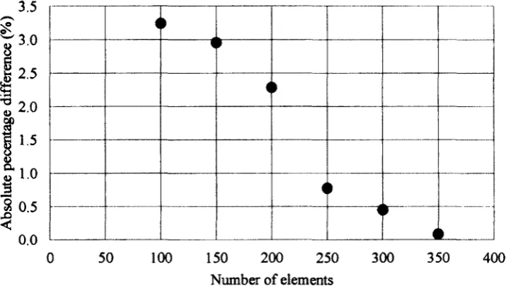
Figure 4-3: Absolute percentage difference vs. Number of elements graph 55
Figure 4-4: COMBIN14 Element geometry (ANSYS 14.0 Documentation) 56
Figure 4-5: Resulting mode shapes 58
Figure 4-6: Sample kinetic energy time-history output 59
Figure 4-7: Kinetic energy time history 61
Figure 4-8: Relation between equivalent first modal damping ratio and damper size at
rd= 0.06 (Rigid damper support and no damper stiffness) 66
Figure 4-9: Effect of damper support stiffness (r<j = 0.06) 69
Figure 4-10: Effect of damper support stiffness (Ks = 52.2, Td = 0.06) 69
Figure 4-11: Effect of damper support stiffness (Ks = 35.0, Tj = 0.06) 70
Figure 4-12: Effect of damper support stiffness (Ks = 17.5, Td = 0.06) 70
Figure 4-13: Effect of damper support stiffness (Ks = 14.3, Ta = 0.06) 71
Figure 4-14: Effect of damper support stiffness (Ks = 8.3, Ta = 0.06) 71
Figure 4-15: Effect of damper stiffness (Ta = 0.06) 73
(Kd = 0.05, rd = 0.06) 79
Figure 4-17: Combined effect of damper stiffness and damper support stiffness
(IQ - 0.10, Td = 0.06) 80
Figure 5-1: Experimental and numerical results (4%L, kd = 0) 82
Figure 5-2: Experimental and numerical results (6%L, ka = 0) 82
Figure 5-3: Experimental and numerical results (10%L, kd = 0) 83
Figure 5-4: Experimental and numerical results (4%L, kd ^ 0) 84
Figure 5-5: Experimental and numerical results (6%L, kd 0) 84
Figure 5-6: Experimental and numerical results (10%L, kd # 0) 85
Figure 5-7: Reduction factor comparison (kd = 280 N/m) 86
Figure 5-8: Reduction factor comparison (kd = 600 N/m) 86
Figure 5-9: Graphical representation of Eq. (5.1) 90
Figure 5-10: Td = 0.04, Kd = 0 91
Figure 5-11: Td = 0.04, Kd = 0.03 92
Figure 5-12: Td = 0.04, Kd = 0.07 92
Figure 5-13: Td = 0.06, Kd = 0 93
Figure 5-14: Td = 0.06, Kd = 0.05 93
Figure 5-15: Td = 0.06, Kd = 0.10 94
Figure 5-16: rd = 0.10, Kd - 0 94
Figure 5-17: Td = 0.10, Kd = 0.08 95
Figure 5-18: Td = 0.10, Kd = 0.17 95
Figure 5-19: Rigid damper support stiffness 97
Figure 5-20: Graphical representation of Eq. (5.2) 100
Figure 5-22: Td = 0.04, Kd = 0.03 102
Figure 5-23: rd = 0.04, Kd = 0.07 102
Figure 5-24: Td = 0.06, Kd = 0 103
Figure 5-25: Td = 0.06, Kd = 0.05 103
Figure 5-26: Td = 0.06, Kd = 0.10 104
Figure 5-27: rd = 0.10, Kd = 0 104
Figure 5-28: rd = 0.10, Kd = 0.08 105
Figure 5-29: rd = 0.10, K<, = 0.17 105
Figure 5-30: Rigid damper support stiffness 107
Figure D-1: Relation between equivalent first modal damping ratio and damper size at
Td = 0.04 (Rigid damper support and no damper stiffness) 125
Figure D-2: Effect of damper support stiffness (Td = 0.04) 126
Figure D-3: Effect of damper support stiffness (Ks = 35.0, Td = 0.04) 126
Figure D-4: Effect of damper support stiffness (Ks = 23.3, Td = 0.04) 127
Figure D-5: Effect of damper support stiffness (Ks = 11.7, rd = 0.04) 127
Figure D-6: Effect of damper support stiffness (Ks = 9.6, Td = 0.04) 128
Figure D-7: Effect of damper support stiffness (Kg = 5.5, Td = 0.04) 128
Figure D-8: Effect of damper stiffness (Td = 0.04) 129
Figure D-9: Combined effect of damper stiffness and damper support stiffness
(Kd = 0.03, rd = 0.04) 129
Figure D-10: Combined effect of damper stiffness and damper support stiffness
(Kd = 0.07, Td = 0.04) 130
Figure D-11: Relation between equivalent first modal damping ratio and damper size at
Figure D-12: Effect of damper support stiffiiess (r d = 0.10) 131
Figure D-13: Effect of damper support stiffness (Ks = 87.5 rd = 0.10) 132
Figure D-14: Effect of damper support stiffness (Ks = 58.3, rd = 0.10) 132
Figure D-15 : Effect of damper support stiffness (Ks = 29.2, r<i = 0.10) 133
Figure D-16: Effect of damper support stiffness (Ks = 23.9, rd = 0.10) 133
Figure D-17: Effect of damper support stiffness (Ks = 13.8, rd = 0.10) 134
Figure D-18: Effect of damper stiffiiess (rd = 0.10) 134
Figure D-19: Combined effect of damper stiffness and damper support stiffness
(Kd = 0.08, rd = 0.10) 135
Figure D-20: Combined effect of damper stiffness and damper support stiffiiess
List of Tables
Table 3-1: Damper stiffness spring properties 27
Table 3-2: Damper support stiffness spring properties 27
Table 3-3: Damper-stiffness combinations 30
Table 3-4: Maximum displacement values for each tested excitation frequency 34
Table 3-5 Summary of the sample experimental data set 36
Table 3-6: Tested stiffness combinations 36
Table 3-7: Summary of modal damping ratios (%) 48
Table 3-8: Absolute percent different between current study results and those from
literature (%) 48
Table 3-9: Experimental modal damping ratios (%) (4%L, ks = rigid) 50
Table 3-10: Modal damping reduction factor comparison 51
Table 4-1: Peak kinetic energy values 62
Table 4-2: Parameter values used in the numerical study 64
Table 4-3: Numerical simulations cases 64
Table 4-4: Current study modal damping ratios (rd = 0.06) 75
Table 4-5: Comparison of modal damping ratio reduction factor 76
Table 4-6: Optimum nondimensional damping parameters
(testing case 4 of the current study) 77
Table 4-7: Maximum achievable damping ratio (%)
Chapter 1; Introduction
1.1 Background
Cable-stayed bridges are commonly used in civil infrastructure. Their economic design, utility, and pleasing aesthetics have led to their use over unprecedented span lengths. The main span of Sutong Bridge in China, for example, is over a kilometer long and is currently the longest in the world. As bridge spans increase, so must their stay cables, which loose rigidity with length. The longest cable on the Sutong Bridge has a length of 580 meters. Due to their low inherent damping, which is often less than 1%, and low natural frequencies, stay cables are particularly sensitive to excitations by various dynamic sources. Violent, large amplitude vibrations of stay cables have been observed on bridge sites, and are of concern both for the healthy maintenance of the structure and for the bridge users. Excessive cable vibrations may result in fatigue failure at the cable-deck or cable-tower connections and/or the deterioration of the cable corrosion mechanism. The source of stay cable vibration is an area of study that is important to ensure the safety of the bridge. To date, a number of vibration mechanisms have been identified as potentially harmful to bridge stay cables. The primary sources of vibration are from rain-wind-induced vibration, vortex-induced oscillation, high-speed vortex excitation, wake galloping, galloping of dry-inclined cables, and parametric excitation.
1.2 Types of cable excitation
Bridge in Japan (Hikami and Shiraishi, 1988). Experimental and analytical studies as well as field monitoring programs were carried out to study the mechanisms associated with this phenomenon (Flamand, 1995; Main and Jones, 2001; Kumarasena et al., 2007; Ni et al., 2007; Taylor and Robertson, 2010; Wang and Hou, 2011). The circular cross-section of the cable is altered with respect to oncoming wind when rain water droplets rest on the cable. This results in an unstable aerodynamic force acting on the cable and, when the droplet oscillates at the natural frequency of the cable, the cable resonates and exhibits large vibrations.
Vortex-induced vibration occurs when wind is acting in the direction perpendicular to the axis of the cable. K6rman vortices shed alternatively from either side of the cable, generating an oscillating force perpendicular to the direction of the wind (towards the cable) which induces cable vibration. If this force oscillates at a frequency near the natural frequency of the cable, resonance occurs which leads to large amplitudes of cable motion. Vortex shedding can be "locked-in" to a resonant frequency for a period when excitation wind speeds have been exceeded. These vibrations generally occur at low wind speeds and have a vibration amplitude response of approximately one cable diameter (Kumarasena et al., 2007; Zuo et al, 2008).
Wake galloping generally occurs when cables are in the wake of other structural elements such as other cables, bridge towers, and nearby buildings. When cables move in and out of a wake, they experience a change in the speed of wind and increased turbulence and they may begin to oscillate. If this oscillation frequency nears the natural frequency of the cable, resonance will occur. Wake galloping may be most easily avoided by installing cables in a properly spaced configuration so they will not be influenced by each other's wakes, as well as minimizing wakes generated from nearby construction (Kumarasena et al., 2007).
Galloping of dry inclined cables occurs in the critical Reynolds number range and has only been observed experimentally; there are no confirmed cases from the field to date. In the lab, vibration was observed when the angle between the cable axis and the wind was 60° or between 75° - 90°. It was found that the mechanism of this type of vibration can be explained by the Den Hartog criterion, but its full mechanism is still not clearly understood (Cheng et al., 2008b).
Parametric excitation occurs when bridge stay cables are forced to vibrate as a result of the motion of the bridge tower or bridge deck. Traffic live load, ground motion (earthquake), and wind are some examples of what may cause the bridge superstructure to move. This movement causes stay cable anchorage points to displace vertically (deck
anchorage) or horizontally (tower anchorage), causing a fluctuation in the tension
1.3 Vibration mitigation techniques
To suppress unfavorable cable motions, various vibration controlling means have been proposed. They can be generally categorized as aerodynamic type and mechanical type.
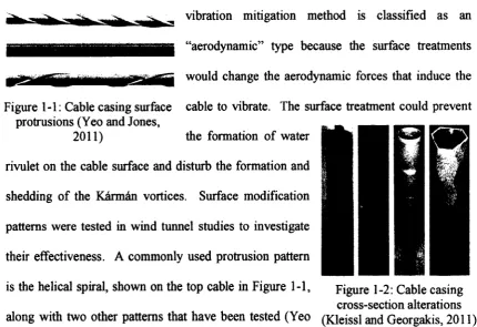
The alteration of the cable casing surface has proven to be an effective measure in controlling both rain-wind-induced vibration as well as vortex-induced vibration. This vibration mitigation method is classified as an "aerodynamic" type because the surface treatments would change the aerodynamic forces that induce the Figure 1-1: Cable casing surface cable to vibrate. The surface treatment could prevent
protrusions (Yeo and Jones,
2011) the formation of water
rivulet on the cable surface and disturb the formation and shedding of the K£rm£n vortices. Surface modification patterns were tested in wind tunnel studies to investigate their effectiveness. A commonly used protrusion pattern
is the helical spiral, shown on the top cable in Figure 1-1, Figure 1-2: Cable casing
The mechanical type of vibration control includes the use of cross-ties, which would increase the in-plane stiffness and thus the natural frequency of cables; and external dampers, which would directly increase damping in the cable.
Cross-ties are transverse cable connectors that connect several stay cables together to increase the overall stiffness and damping of the entire cable network. The points of tie connection limit the motion of the stays, decreasing their effective length and increasing cable in-plane stiffness, which tends to increase the natural frequencies of the cables. Environmental cable excitation is generally most critical in the lower modes of vibration. Increased cable natural frequencies help to avoid increased dynamic response at resonance in these critical lower modes. Both experimental and numerical work (e.g. Yamaguchi and Nagahawatta, 1995; He et al., 2010; Caracoglia and Jones, 2005) have shown that flexible cross-ties are more effective than their stiff counterparts because flexibility allows for energy dissipation within the cross-ties, and that some prestress should be applied to the cross-ties when they are installed. However, segmenting the cable with the ties tends to generate intense local vibrations that are not desirable. This method of vibration mitigation has been successfully used on several bridges, for example, the Fred Hartman Bridge in Texas, USA (Caracoglia and Jones, 2005), and the Dames Point Bridge in Jacksonville, Florida, USA (Kumarasena et al., 2007).
particles in the damper in the direction parallel to an applied magnetic field. They have been explored primarily through semi-active control (Johnson et al., 2007), and passive control (Cho et al., 2005). A newly proposed method of vibration contol changes the boundary condition of the classic cable system: one end of the cable is no longer fixed. The support is flexible and has both stiffness and damping in the direction of cable vibration, which may reduce vibration displacement more effectively than a passive damper (Hwang et al., 2009). Viscous dampers are the most commonly used mechanical type. They are being used on the Fred Hartman Bridge in the USA, the Brotonne Bridge in France, and the Aratsu Bridge in Japan. Design tools have been proposed and developed for their application (e.g. Pacheco et al., 1993; Tabatabai and Mehrabi, 2000; Cheng et al, 2010). Improvements to the classic viscous damper have been attempted recently with adjustable fluid dampers (Xu and Zhou, 2007). They use shape memory alloy to optimize the damper performance.
Often overlooked, however, is the effect of damper and damper support stiffness in the viscous damper design. Practical design tools must include these parameters in order to predict accurately the additional damping from the damper. Without considering these factors, damping may be overestimated in design and cables in the field may not receive adequate damping as expected, which may leave the bridge structure vulnerable to dynamic excitation.
1.4 Motivations
performance of a viscous damper, and their combined effect has rarely been investigated. The very few existing studies which explored this issue indicated that both damper and damper support stiffness would have a sizeable effect on the accurate prediction of the system damping ratio.
The lack of study in the area of how damper stiffness and damper support stiffness would affect damper efficiency was the motivation for the current work, which included the construction of an experimental study and a finite element analysis of the dynamic behaviour of a cable-damper system while including damper and damper support stiffness properties. The impacts of these two parameters on the damper performance were investigated separately as well as in combination. This study has not only confirmed the trends currently documented, but it has extended their practicality to the actual damper design by proposing approximations for the optimum damper size and its corresponding maximum equivalent first modal damping ratio.
1.5 Objectives
The objectives of this study were thus proposed to be:
1. Design a linear viscous damper that allows for adjustable damper stiffness and support stiffness.
2. Design the calibration system for the damper.
3. Conduct cable forced vibration tests to observe the following: a. the effect of damper support stiffness on cable damping ratio
4. Develop a finite element model of the cable-damper system including damper stiffness and damper support stiffness. The model was developed using the ANSYS commercial software. The energy-based method proposed by Cheng et al. (2010) was used to calculate the damping ratio of the system.
5. Compare experimental and numerical results, as well as those reported in the literature.
Chapter 2: Literature Review
A common simplification in the analysis of a cable-damper system has been to idealize the cable as a taut string. Therefore, cable sag (inclination) and bending stiffness are neglected. This assumption has often been used in analytical studies, such as those that use complex eigenvalue analysis to estimate the additional damping expected in different modes of vibration from a linear viscous damper.
Kovacs (1982) identified the existence of an optimum viscous damping coefficient using the semi-empirical approach and developed an analytical equation estimating its value, based on the two extremes of cable damping: no damping and a damper with infinite damping capacity, which will act as a rigid support. This research analyzed only the first mode of cable vibration, although it has the potential of being extended to higher modes.
A universal damping estimation curve was subsequently developed by Pacheco et al. (1993), also based on eigenvalue analysis using the taut cable assumption. This curve, shown in Figure 2-1, can be used for a practical range of stay cables and linear viscous dampers, and it assesses the optimal size and location of a damper needed for controlling cable vibration in a specific mode in which the maximum amount of additional damping must be provided. In addition, this curve can further estimate the additional damping to be had in other modes based on the initial damper design developed from the curve. Modal damping ratio is plotted on the y-axis and the non-dimensional damper coefficient
is potted on the x-axis, where ft is the modal damping ratio in the Ith mode of vibration, xc
m is the mass per unit length of the cable, &)0x is the fundamental natural frequency of the
cable, and i is the mode number. This curve can be used for the first six modes of cable
vibration and it has increased usefulness over previous work because of its simplicity in application. An analytical solution representing the universal estimation curve has also been developed. It was proposed by Krenk (2000) that maximum additional damping that can be achieved from a linear viscous damper could be approximated simply as £ =
xc/ 2 L .
• | • I • | ' I I I ' I r| • | M ' I ' I ' I ' I ' I ' I ' I 1 1 '"I ' I
j . . . . . i '•••£•*'•? " " i * " " I "
*e 0.3
p....
0 0.1 02 0.3 0.4 0.5 0.6 0.7 0.8 0.9 1.0
C mLcOoj L
Figure 2-1: Universal damping estimation curve (Pacheco et al., 1993)
was analyzed as a "clamped case" and analytically described by a clamping ratio, which was seen to increase with mode number, for a particular damping coefficient. This means that the damper acts in a more rigid manner for higher cable vibration modes, and confirms that this type of damper may only act optimally for one mode, because its effectiveness decreases for other modes. This optimal mode must be known before the damper is designed, and must be designed on a case-by-case basis for each cable in question, which may not be economically practical in design. It is worth pointing out that, though not optimal, a linear viscous damper may offer some damping effect to other vibration modes.
An analytical comparison between linear and nonlinear viscous dampers has been done by Main and Jones (2002) using the taut cable assumption. A universal damping estimation curve for a nonlinear damper was developed. The behavior of a nonlinear viscous damper can be generally described as exerting a force, proportional to the velocity of the cable, raised to some positive exponent. The use of this type of damper might be an improvement over the linear viscous damper because its efficiency is largely dependent on the amplitude of cable oscillation, and is less sensitive to mode number. The damper performs optimally in modes that experience oscillations in the vicinity of the design amplitude. Specifically, it was found that a nonlinear viscous damper with the exponent of V2 was completely independent of mode number and was equally effective at the same amplitude of vibration oscillation, regardless of the mode. This extends the design of dampers beyond a specific mode of vibration.
P\ **_ FUmant 2 P}
*1-^ Element 1 — JpSem3^ associated complex eigenvalue
- h—L=r 12 inr—r'}—" formulation have been extended to the
Damper 1 \\\\\ Damper 2
Figure 2-2: Taut string-two damper model tw0 damper case> ^ illustrated in
(Caracoglia and Jones, 2007) ^ tt . ,
Figure 2-2. Universal damping
estimation curves (comparable to the taut-string, single damper curve) were generated by Caracoglia and Jones (2007) for the two damper case as well. It was found that the modal damping of the damped cable was improved when the dampers were installed at opposite ends of the cable, but worsened when located at the same end due to their interaction. The latter would actually increase the stiffness at that end of the cable.
Tabatabai and Mehrabi (2000) studied the dynamic behaviour of a damped flexible cable by including the sagging and bending stiffness of the cable in the formulation. A notable conclusion was made that bending stiffness has a considerable effect on the obtainable damping ratio that can be achieved by a mechanical viscous damper, and that the taut cable approximation is likely to overestimate the obtainable damping ratio. Design equations / methods for damper design have been proposed which include bending stiffness but restrict damper location to the vicinity of the cable end.
Cable sag, often analytically expressed by the inextensibility parameter (A2) was
initially proposed by Irvine and Caughey (1974). It is defined as the ratio of the stiffness of an ideal massless cable to that of an actual sagging cable. The sagging effect was found to be significant primarily in the first mode of vibration for cables with an inextensibility parameter greater than one. The universal damping estimation curve proposed by Pacheco et al. (1993) was deemed valid only for short to medium length damper analytical model and the
cables, where sag can justifiably be neglected. Xu and Yu (1998), as well as Tabatabai and Mehrabi (2000), developed curves, similar to the universal damper design curve, to determine the maximum damping ratio and the optimum damper size while considering the cable sagging effect for the first mode of cable vibration and beyond.
Energy-based methods have been explored to evaluate the additional damping provided by an attached viscous damper. Jiang (2006) used the kinetic-energy decay ratio of a freely vibrating cable, obtained from a finite element model developed using the ANSYS commercial software, and converted it into equivalent Rayleigh damping.
Cheng et al. (2010) developed a mathematical equation based on the kinetic energy decay time-history of a freely vibrating damped cable to evaluate the additional damping provided by an attached viscous damper. The time-history response was obtained from numerical simulations of a freely vibrating cable damper system developed using the ABAQUS commercial software. This work expanded on the previous studies by not only including the sag and flexural rigidity of the cable, but also lifting the restriction on the damper installation location in the application.
Xu et al. (1999) conducted both free and forced vibration tests on a cable-damper system, with varying cable tension to simulate a range of sag conditions. The existence of an optimal damper coefficient that can reach a maximum modal damping ratio for a given damper location has been confirmed. Large-amplitude force-controlled vibration tests revealed non-linear vibration of an undamped cable, while the linearity was restored in the three lowest modes of vibration with the use of an oil damper. Out-of-plane vibration was also observed during these tests near the first in-plane natural frequency of the cable because of its proximity to its first out-of-plane natural frequency, which was thought to have generated internal resonance. In the experiment, the oil damper was found to be able to extinguish the out-of-plane vibration in the first mode, while effectively mitigating the in-plane vibration.
Field observations evaluating the performance of linear viscous dampers were conducted by Main and Jones (2001) on the Fred Hartman Bridge in Texas, USA, where two dampers were installed on two different stay cables. The dampers were found to be effective in mitigating cable vibrations that were identified to have stemmed from vortex-and rain-wind-induced excitations. After installing the dampers, not only the amplitude of cable vibration but also the acceleration of cable motions were decreased significantly. It was also observed that the damper forces were the greatest when the wind was in the same direction as the cable was declining.
cable damping ratio. However, installing the two dampers at the same end of the cable will reduce the cable damping ratio.
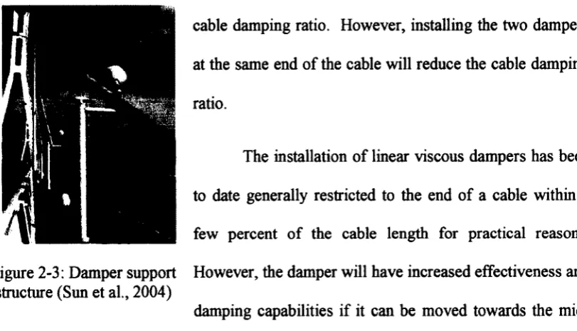
The installation of linear viscous dampers has been to date generally restricted to the end of a cable within a few percent of the cable length for practical reasons. However, the damper will have increased effectiveness and damping capabilities if it can be moved towards the mid-span of the cable. In field applications, this may require a damper support structure to allow the damper to be installed beyond its conventional position, as shown in Figure 2-3. It is worth noting that none of the studies reviewed above considered the stiffness of the damper itself and the support in the formulation. These could have considerable impact on the efficiency of the damper.
A few studies addressed the issue of damper stiffness and damper support stiffness. Zhou (2005) used complex modal analysis to develop an equation for the optimal damper size, which included damper stiffness. It was found that as the non-dimensional damper stiffness increased, the optimal damper size would increase linearly.
Xu and Zhou (2007) developed an analytical formula using the taut cable assumption for the cable damping ratio using an adjustable fluid damper. This damper type acts as a passive fluid damper after the optimum damping coefficient is found through application. The formula represented the adjustable fluid damper using the Maxwell model, which can be described as a dashpot connected in series with a spring. Figure 2-3: Damper support
An additional spring was connected in series with the damper spring to represent support stiffness. The cable damping ratio was represented as a function of damper support stiffness; an increase in damper support stiffness increased the cable damping ratio.
Fujino and Hoang (2008) analytically derived an asymptotic formula for the modal damping of a cable, which included cable sag, flexural rigidity, and damper support stiffness. In the formula, the influencing factors were expressed as modification / reduction factors, which can be used conveniently in practical damper design. This study confirmed that, for cables with a small sag parameter, sagging effect was significant only
for the 1st symmetric mode of cable vibration and that the influence of cable flexural
rigidity was apparent in all modes of interest. Damper support stiffness was found to be independent of the mode of cable vibration and to have a significant effect on the maximum damping capability of the damper. With the increase of damper support stiffness, the cable damping ratio increases. Damper design equations including the damper support stiffness were proposed.
The analytical work by Huang and Jones (2011) has led to the development of universal damping estimation curves for predicting modal damping ratio of a damped cable by including the effect of damper support stiffness, although the taut cable assumption was used in their formulation. In this study, a decrease in damper support stiffness was also found to decrease additional damping from an attached linear viscous damper.
on the taut string assumption. An increased damper stiffiiess and decreased damper support stiffness were each found to independently decrease the maximum obtainable cable damping ratio. Efficiency factors were proposed, which were defined as the ratio of actual additional damping from experimental results to the analytically calculated results based on ideal linear viscous damper theory.
Huang (2011) conducted an experimental work focusing specifically on the effect of damper stiffness on the efficiency of a linear viscous damper in suppressing cable vibrations. Springs were installed between a model cable and a linear viscous damper to simulate the damper stiffness. Results indicated that the existence of damper stiffiiess would reduce the effectiveness of a damper.
Chapter 3: Experimental Study
An experimental study was carried out to investigate the dynamic behavior of a cable-damper system. This chapter will include a detailed description of the experimental setup, the equipment, and the testing procedures that have been used, as well as the experimental results. An existing experimental setup, developed by Huang (2011), was modified to be used for the current study. This experimental study was set up in room B-19 in Essex Hall at the University of Windsor, Ontario, Canada.
3.1 Experimental setup
A steel wire cable was used to model a bridge stay cable and it was mounted horizontally between two steel columns. A sketch of the experimental setup is shown in Figure 3-1.
£
Loaded
Acceferocneter
I |
\\
Hyfrauic \ •
hand pomp / / / / ////
*
Figure 3-1: Sketch of experimental setup
One end of the cable was attached to a load cell for measuring the pretension in the cable, and the other end was attached to a hydraulic pump for applying tension in the cable. The cable had a span length of 9.33 m (mounted into position), a nominal diameter of 4.65
mm, a unit mass of 0.092 kg/m, and a nominal moment of inertia of 15.8 mm4. The
This range is high enough to avoid too little tension in the cable, which would cause the cable to be slack, and low enough to avoid too much tension, which would cause the vibrating cable to exhibit elliptical motion. The pretension in the cable used for this experimental study was 3200 N. The natural frequency of the model cable was lowered to approach that of an actual bridge stay cable by adding 20 evenly spaced 50 gram mass blocks to increase its unit mass. The resulting unit mass of the cable was 0.2 kg/m. The
first natural frequency of a cable (/i) can be predicted using the formula: fi =
1/(2lS)yjT/m, where L = cable length (m), T = cable pretension (N), m = cable unit mass (kg/m). The resulting natural frequency of the cable, after the addition of the mass blocks, is predicted to be 6.78 Hz. In the lab, the natural frequency of the cable was found to be approximately 7.0 Hz.
Figure 3-2: Universal Flat Load Cell
An Enerpac hydraulic steel hand pump, shown in Figure 3-3, was installed at the opposite end of the cable from the load cell to apply pretension to the cable. The unit, model number PH-84, has a maximum pressure rating of 10,000 psi. In this experiment, the hydraulic pump was setup to exert a pretension of 3200 N to the cable. This value was measured by the load cell located at the opposite end of the cable.
An accelerometer was placed at the mid-span of the cable to monitor the first modal response of cable vibration. It was placed on the very top of the cable cross-section in order to record only the vertical motion. Real time data was collected using the Astrolink Xe data acquisition and control software. The data was monitored to make sure that the wave-form acceleration data collected was symmetric, which indicated that the unit is properly placed at the top of the cable and is receiving data from only the vertical direction of motion. The accelerometer used, model number 352A24, was purchased from Dalimar Instruments and has a testing range of 1 - 8000 Hz. The testing range used in this experimental study was 6-8 Hz.
Figure 3-4: Smart Shaker
An HP signal generator, model number 33120A, was used to generate the dynamic excitation functions to control the dynamic shaker. This unit, shown in Figure 3-5, has the ability to generate many output functions including sine, square, triangle, and ramp, among others. The sinusoidal output function was used in this experiment. The
signal generator can generate this output function in a frequency range of 1 - 15 MHz.
The data acquisition recorder used was AstroDAQ Xe from Astro-Med, Inc. The unit, part number 22834-513, connects to a computer through a USB 2.0 interface and has eight input channels. Both the load cell and the accelerometer were connected to this data recorder, shown in Figure 3-6. The software that was used with this recorder was the AstroLINK Xe data acquisition and control software, also from Astro-Med, Inc. The software, part number 22834-514, can record data at frequencies up to 200,000 Hz. In this experiment, a sampling frequency of 1000 Hz was used. The Realtime mode in the
software was used to monitor and capture real-time acceleration data from the
accelerometer. The review mode in the software was used to review and save data previously captured.
3.2 Damper design and calibration
A passive linear viscous damper was used in this experimental study. This damper type provides a dissipative damping force generated from the pressure difference from a piston moving through a viscous fluid. The damper used in this study was designed to have variable damper stiffness and support stiffness. It was also imperative that all energy in the system be affected only by the damper and stiffness components (no loss of energy due to friction), to result in an accurate cable damping ratio. A photograph of the damper designed for this experimental study is shown in Figure 3-7.
The designed damper has the following main components:
1. A plastic container holds the viscous fluid. It is open at the top and it has an inner diameter of 100 mm. The bottom of the container has 12 holes carved into it to fit the support springs. Figure 3-8 shows a sketch of the damper container.
v i
Figure 3-8: Damper container sketch
O I3mr Typ
O O
4 8 rnn
•Squate
Figure 3-9: Damper block sketch
2. SYNTON PAO 100, produced by Chemtura Canada Co. and obtained from Commonwealth Oil, was used as the viscous fluid for this damper. It has a kinematic viscosity at 40°C of 1279.51 centistokes (cSt).
increase the damper damping coefficient. It has a mass of 80.78 g. Figure 3-9 shows a sketch of the damper block.
4. A plastic stick connects the block to the cable. It screws into the center of the block and attaches to the cable through two aluminum pieces that fit around the cable cross-section. The stick and aluminum pieces have a mass of 26.10 g. Figure 3-10 shows a picture of the damper block connected to the stick and aluminum pieces.
5. Two sets of two springs were used to simulate the damper stiffness. They are connected to the damper container through two aluminum hooks screwed into the top surface edges of the container, directly across from each other, and they are connected to the cable directly. The stiffness of the springs was
measured experimentally in the lab. The springs were obtained from
McMaster-Carr and have the following properties: Figure 3-10: Damper block,
Table 3-1: Damper stiffness spring properties
Spring Part No. 9654K53 9654K812
Stiffness (N/m) 140 300
Spring type Steel Extension Spring Steel Extension Spring
6. Two sets of six springs were used to simulate the damper support stiffness. They sit in an acrylic base plate that has holes carved out to fit their cross-section. The base of the plastic damper container rests on the springs. It has holes carved out of its base to fit the springs. The stiffness of the springs was
measured experimentally in the lab. The springs were obtained from
McMaster-Carr and have the following properties:
Table 3-2: Damper support stiffness spring properties
Spring Part No. 9434K147 9434K135
Stiffness (N/m) 5780 7880
Spring type
Music wire precision compression spring,
zinc-plated
Music wire precision compression spring,
zinc-plated
7. An acrylic base plate was designed to accompany the damper and allow for
varying support stiffness. It has two sets of six holes carved into it
symmetrically. Each set of six holes accommodates one set of support stiffness springs. The two sets of support stiffness springs can be used either independently or in combination. The base plate can also be directly attached to the damper to simulate an infinitely stiff support.
block and stick) as it moves through the damper viscous fluid under constant applied forces. The LVDT cylinder was placed on the lid of an acrylic structure, shown in Figure 3-11, which has an opening in its side to allow for the raising and releasing of the damper piston.
Figure 3-11: Acrylic calibration unit
has a unit of Ns/m. The applied force during calibration includes the weight of the damper acrylic block, the plastic stick and the attached aluminum pieces, the mass blocks used, the screws to attach the aluminum pieces together, and the LVDT stick. As the damper piston is released, each time with different mass blocks installed, the data acquisition software records the velocity of the LVDT stick. The relation between the applied force and the damper piston velocity, illustrated in Figure 3-12, was produced from calibration results and linear regression analysis. The slope of this force-velocity curve is the damper coefficient with the unit of Ns/m. The damper in this experimental study had a damping coefficient of 32.2 Ns/m.
2.5
2
g '
51
o 1tu 1
0.5
0
0 0.01 0.02 0.03 0.04 0.05 0.06 0.07
Velocity (m/s)
Figure 3-12: Force vs. Velocity calibration graph
3.3 Forced-vibration tests
Forced-vibration tests were performed to observe vertical cable motion under
varying excitation frequencies. The combinations of damper stiffness and damper
support stiffness that were tested are described in Table 3-3.
y = 32.237x +0.2358
• Data Points
Table 3-3: Damper-stiffness combinations
Damper coefficient (Ns/m) 32.2
Damper support stiffness
(N/m) Infinite 82000 47300
Damper stiffness (N/m) 0 280 600 0 280 600 0 280 600
The following describes the experimental testing procedures that were followed:
1. Find the first natural frequency of the cable (to the nearest 0.05 Hz) by adjusting
the excitation frequency of the shaker through the signal generator. The
maximum cable response from the accelerometer data can be captured in the Realtime mode of the AstroLINK Xe software (i.e. resonance). The experimental value of the first natural frequency of the cable will be slightly higher than that estimated theoretically because the installation of the shaker decreases the effective length of the cable.
2. Create a file name for the current test and select the sampling frequency (1000 Hz was used) in the AstroLink Xe software.
3. Set the signal generator to a frequency of 0.5 Hz less than the experimental natural frequency and record the acceleration data. This data file may be subsequently reviewed (in the Review mode) and saved as a Microsoft Excel file.
4. Increase the signal generator frequency by 0.05 Hz for each test, up to (/i + 0.5) Hz. Each damper-stiffness combination will therefore be tested at 20 frequency values.
-0.6 H z ) - ( f x + 0.6 H z ) and had a filter order of two. The acceleration data was subsequently converted to displacement data using a Fourier Transform and the Matlab commercial software. With this displacement data, the half-power method was used to determine the cable-damping ratio of the tested system by plotting the frequency-response curve.
A sample data set will be presented to fully illustrate the experimental procedure. The sample data set will have the damper located at 10% of the cable length, with a damper stiffness of 280 N/m and a damper support stiffness of 47300 N/m.
First, a pretension of 3200N was applied to the cable using the hydraulic hand pump. The value of pretension was measured by the load cell, which was connected to the AstroDAQ Xe data acquisition system, and observed in the Realtime mode of the AstroLINK Xe software. The shaker was installed at 5% of the cable length, at the opposite end from the load cell. It was set to its maximum amplitude and connected to the signal generator. The signal generator was set to a sinusoidal output function. The accelerometer was installed at the mid-span of the cable, on the top of the cable cross-section. It was also connected to the data acquisition system.
parallel and their combined stiffness is a direct addition of each spring stiffness, which results in a damper support stiffness of 47300 N/m. The damper container is filled with the viscous fluid, SYNTON PAO 100, and the container is placed on the support springs. The top of the support springs fit into the holes in the damper container base. The damper block is attached to the plastic stick and placed in the damper container. The plastic stick is connected to the cable through its attached aluminum pieces, which are screwed together with the cable in between them. The two damper stiffness springs, each with a stiffness of 140 N/m, are installed in parallel. The bottom of each spring is attached to an aluminum hook, on each side of the container. The top of each spring is hooked directly onto the cable. Their combined stiffness is 280 N/m.
The fundamental frequency of the cable is then found in the experiment by adjusting the output frequency on the signal generator. The fundamental frequency is found to be approximately 7.20 Hz by qualitatively observing the maximum cable
response at this excitation frequency. The shaker and damper attachments caused the
fundamental frequency to increase slightly. The testing frequency range was 0.5 Hz below the fundamental frequency to 0.5 Hz above it, therefore 6.70 - 7.70 Hz. The signal
generator was set to 6.70 Hz. The sampling frequency was set to 1000 Hz. The
AstroLINK Xe software was used to capture the data over a time period of 12 seconds. The data was then reviewed in the Review mode and saved an excel file for further
processing. The signal generator output frequency was increased by 0.5 Hz and the
The following details the data processing of the sample data set. The acceleration data from the first data file (6.70 Hz) was brought into Matlab; it was represented by the variable "b". The Butterworth filter was designed in Matlab using the "Filter Design & Analysis Tool". It was of Bandpass response type and a filter order of two. The filter was represented by the variable "Hd". An M-file, designed by Huang (2011) and included in Appendix A, was subsequently used to process the data. This file applies the Butterworth filter to remove higher modes of vibration from the experimental data and it applies Fourier Transform to convert acceleration history data to displacement time-history data. The M-file produces a graphical output of the displacement time-time-history data, shown in Figure 3-13. The maximum displacement is found using the "Data Cursor" tool, which displays data values interactively. The maximum displacement value for this data set was found to be 0.6133 cm.
01 0« 04
0 2
-0 2
•04
•Ot
•Ot
0 2 4 6 « 10 12
Tim«<S«cond)
Table 3-4: Maximum displacement values for each tested excitation frequency Excitation frequency
(Hz)
Maximum displacement (cm)
6.70 0.6133
6.75 0.6905
6.80 0.8046
6.85 0.9372
6.90 1.090
6.95 1.254
7.00 1.409
7.05 1.545
7.10 1.585
7.15 1.545
7.20 1.444
7.25 1.317
7.30 1.191
7.35 1.065
7.40 0.9495
7.45 0.8478
7.50 0.7586
7.55 0.6841
7.60 0.6178
7.65 0.5622
7.70 0.5108
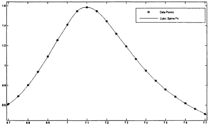
The maximum displacement for each data file was subsequently found. These values are presented in Table 3-4. A variable was created for the excitation frequency (F) and the maximum displacement (D) in Matlab. The Curve Fitting Tool was used to plot maximum displacement (D) in centimeters versus excitation frequency (F) in Hz. The data was fitted with a cubic spline, interpolant type of fit, shown in Figure 3-14. The fitting curve was analyzed using the Analysis Tool, and the displacement was interpolated
at each 0.001 Hz along the fitting curve. The maximum displacement (Dmax) may then be
12
0.1
t r i i i 1 r
O D«t* Points
Cubic Splint Fit
J I I I I I I I I I
<7 «• 63 71 72 73 74 7 5 7e 77
Figure 3-14: Maximum displacement (cm) vs. Excitation frequency (Hz)
The half-power method was subsequently used to calculate the experimental cable-damping ratio. The steps are listed below and a summary of the sample data set is presented in Table 3-5.
1. The maximum displacement was divided by the square-root of two to calculate the half-power points:
Dmax _ 1.58517 cm
__ — = 1.120884 cm
2. The excitation frequencies (on each side of the peak displacement) that correspond to this displacement value were found to be:
Ri = 6.910 Hz
3. The damping ratio was calculated using the following formula:
R2-Ri 7,328Hz - 6.910HZ
5 = „ = „ooo„ , = 0.02936 = 2.936%
R2 t Rj 7.328Hz "I- 6.910Hz
Table 3-5 Summary of the sample experimental data set
Damper location Ld 10% L
Damping coefficient c (Ns/m) 32.2
Damper stiffness kd (N/m) 280
Damper support stiffness ks(N/m) 47300
Damping ratio £ (%) 2.936
3.4 Experimental results
Table 3-6 summarizes the combinations of damper stiffness and damper support
stiffness that have been tested. The damper was installed at 4%L, 6%L, and 10%L. The
experimental results for each damper location are presented graphically in Figures 3-15, 3-16, and 3-17, respectively.
Table 3-6: Tested stiffness combinations
Damper damping coefficient c
(Ns/m) 32.2
Damper support stiffness ks
(N/m) Infinite 82000 47300
0.6
0.5
£
0
-
4
*u>o
2 0.3
Q 0.2
0.1
0.0
f
£
1
0 Damper stiffness = 0 N/m
• Damper stiffness = 280 N/m
A Damper stiffness = 600 N/m 0 Damper stiffness = 0 N/m
• Damper stiffness = 280 N/m
A Damper stiffness = 600 N/m 0 Damper stiffness = 0 N/m
• Damper stiffness = 280 N/m
A Damper stiffness = 600 N/m
1
1.6 1.4 1.2 1.0 o '•g ^ 0.8 0.6 0.4 0.2 0.050000 100000 150000
Damper support stiffness ks (N/m)
Figure 3-15: Experimental results (4%L)
200000
• Damper stiffness = 0 N/m
• Damper stiffness = 280 N/m
A Damper stiffness = 600 N/m
50000 100000 150000
Damper support stiffness ks (N/m)
200000
UJ> 0
1
M Q. 0 • A O •- A
f
I
O Damper stiffness = 0 N/m
• Damper stiffness = 280 N/m
A Damper stiffness = 600 N/m O Damper stiffness = 0 N/m
• Damper stiffness = 280 N/m
A Damper stiffness = 600 N/m O Damper stiffness = 0 N/m
• Damper stiffness = 280 N/m
A Damper stiffness = 600 N/m O Damper stiffness = 0 N/m
• Damper stiffness = 280 N/m
A Damper stiffness = 600 N/m
1 4.0 3.5 3.0 2.5 2.0 1 5 Q 1.0 0.5 0.0
0 50000 100000 150000 200000
Damper support stiffness ks (N/m)
Figure 3-17: Experimental results (10%L)
The experimental results given in Figures 3-15, 3-16, and 3-17 show that the effects of damper support stiffness and damper stiffness on the performance of a linear viscous damper are similar at all three tested damper locations. It can be observed from these three figures that the modal damping ratio of the cable-damper system increases as damper support stiffness increases. This is the same trend that has been observed in previous studies (Xu and Zhou, 2007; Fujino and Hoang, 2008; Huang and Jones, 2011). The reason for this behaviour may be attributed to difference in damping force that the damper exerts when it has a rigid support (Figure 3-18) compared to when it has a support with finite stiffness (Figure 3-19). The damping force exerted by the damper may be expressed by the following:
where Fj is the damping force exerted by the damper on the cable (N), c is the damping
coefficient of the damper (Ns/m), VA is the velocity of the node where the damper
connects to the cable (m/s), and VB is the velocity of the node where the damper connects
to its base support (m/s). Nodes A and B are illustrated in both Figures 3-18 and 3-19. In Figure 3-18, a sketch of a damper with a rigid support is shown. For this case, the
velocity of node B (VB) in Eq. (3.1) would be zero because the rigid support is not in
motion. When this is inserted into Eq. (3.1), the value of the damping force becomes the following:
In Figure 3-19, a sketch of a damper with a support of finite stiffness is shown. The
velocity of node B (VB) in this case would be a nonzero value. This results in a smaller
damping force than in the case where the damper has a rigid support. Therefore, a damper with a finite support provides less damping than that with a rigid support.
Fd = cVA (3.2)
\ \
\
\
\\
A
/
/ //
/
Figure 3-18: Sketch of a damper with a rigid support
\
\
\
\
A
/
/
/
/
\
1/The experimental results also show that the modal damping ratio decreases as the damper stiffness increases. This trend, observed by Zhou (2005) and Huang (2011), is reasonable because the existence of the damper stiffness reduces the efficiency of the damper by absorbing part of the energy and converting it to elastic energy. Without damper stiffness, this part of energy would otherwise be transferred to the damper and be dissipated through its damping mechanism. This set of data implies that to achieve the maximum efficiency of a linear viscous damper, preferably, it should be supported on a rigid base, and the stiffness of itself should be negligible.
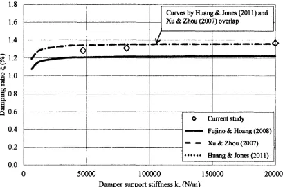
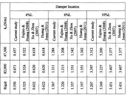
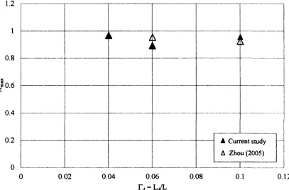
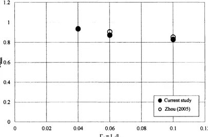
The experimental results obtained have been compared with the existing literature to confirm their accuracy. The studies conducted by Xu and Zhou (2007), Fujino and Hoang (2008), and Huang and Jones (2011) have produced analytical formulae that predict the value of the modal damping ratio of a cable-damper system while including the effect of damper support stiffness. However, the effect of damper stiffness was not considered in these works. These formulae will therefore be used to compare with the zero damper stiffness cases of the current study. The study conducted by Zhou (2005) produced a damper efficiency reduction factor that accounts for the effect of damper stiffness only. The degradation of damper performance caused by the presence of damper stiffness observed in the current experimental study will be compared with the reduction factor calculated using the formula developed by Zhou (2005).
where £ is the nondimensional modal damping ratio of the cable-damper system in the
mode of vibration, xc is the location of the damper, L is the length of the cable, co0i is the
undamped circular frequency of a taut cable in the first mode of vibration, kt is the
nondimensional damping parameter in the P mode of vibration, calculated based on the following:
where c is the damper coefficient. The damper support stiffness is included in the term A,
which is defined as the total relaxation time constant and is a component of the Maxwell model upon which these equations are based. This term may be calculated using the following formula:
where kd is the damper stiffness in series with the damper, and k, is the support stiffness
in series with both the damper and the damper stiffness. For the purpose of comparison with the current results, which only had the damper support stiffness in series with the
damper (damper stiffness was in parallel with the damper), the term c/kj was taken as
zero. In order to utilize Eq.
(3.3)
to compare with the results of the current study, xJLwas taken as
0.04, 0.06,
and0.10
for the4
%L, 6%L, and10%Z,
damper locations,respectively. The values of c, m, L, and
G>
0I
were taken as32.2
Ns/m,0.2
kg/m,9.33
m,and
42.59
radians/s, respectively. The value of k3 was varied from6,300
N/m to200,000
N/m. The value of damper support stiffness used to represent a rigid support was taken as
200,000
N/m. This is appropriate because this value is significantly larger than the valuesused for the finite support stiffness. The formula developed by Xu and Zhou
(2007)
uses(3-4)
the taut cable assumption. Therefore, cable sag and bending stiffness were neglected. The dashed line in Figures 3-20 to 3-22 portrays the results by Eq. (3.3).
The equation developed by Fujino and Hoang (2008) for evaluating the amount of damping provided by an external linear viscous damper to suppress cable vibrations while considering the damper support stiffness is the following:
Sn „ „ k2nfnsnnn ^
—77 = RsnRf——: _ . 2 , , (3-6)
xc/L k2 + (l + knf) n|nn^
where k = xck/H is the dimensionless damper support stiffness, xc is the location of the
damper, k is the damper support stiffness, H is the chord tension of an inclined cable, and
L is the length of the cable. The terms «/ and nm are the modification factors due to cable
flexural rigidity and sag, respectively, and n„ is a modification factor that includes the
dimensionless damper damping coefficient and its location along the cable length. The values for these modification factors were calculated using the formulae proposed in the
study. For example, when the damper is located at 4%L, r\f and n„ are calculated to be
0.874 and 0.160, respectively. The value of nm was calculated to be equal to one (this
factor is not dependent on the location of the damper). The terms Rm and R/ are the
sag. Since the damper stiffiiess was not included in this formula, only the experimental data points that have zero damper stiffness were used for comparison.
The universal curve equation proposed by Huang and Jones (2011) predicts the modal damping ratio of a cable-damper system by including a flexibility coefficient that takes into account the damper support stiffiiess. The equation has the form of the following;
~ (3.7)
xc/L 1 + (tc2 k)2^2
where k is the nondimensional damping coefficient, which can be expressed as:
k
=akr'(r)
(38)
and C is the effective flexibility coefficient expressed as:
1/Y
?=1+
J;
(3
-
9)
The effective flexibility coefficient includes a nondimensional spring stiffness parameter
X which is expressed as:
* = ¥ (3'9)
where k is the damper support stiffness, L is the cable length, and H is the cable tension