Study of the Viscometric and Volumetric Properties of Multicomponent Regular Liquid Systems at Different Temperature Levels

(1)

Scholarship at UWindsor

Electronic Theses and Dissertations Theses, Dissertations, and Major Papers

2012

Study of the Viscometric and Volumetric Properties of

Multicomponent Regular Liquid Systems at Different Temperature

Levels

Nidal Hussein University of Windsor

Follow this and additional works at: https://scholar.uwindsor.ca/etd

Recommended Citation Recommended Citation

Hussein, Nidal, "Study of the Viscometric and Volumetric Properties of Multicomponent Regular Liquid Systems at Different Temperature Levels" (2012). Electronic Theses and Dissertations. 8028.

https://scholar.uwindsor.ca/etd/8028

This online database contains the full-text of PhD dissertations and Masters’ theses of University of Windsor students from 1954 forward. These documents are made available for personal study and research purposes only, in accordance with the Canadian Copyright Act and the Creative Commons license—CC BY-NC-ND (Attribution, Non-Commercial, No Derivative Works). Under this license, works must always be attributed to the copyright holder (original author), cannot be used for any commercial purposes, and may not be altered. Any other use would require the permission of the copyright holder. Students may inquire about withdrawing their dissertation and/or thesis from this database. For additional inquiries, please contact the repository administrator via email

(2)

Multicomponent Regular Liquid Systems at Different Temperature

Levels

By

Nidal Hussein

A Dissertation

Submitted to the Faculty of Graduate Studies

through the Environmental Engineering Program

in Partial Fulfillment of the Requirements for

the Degree of Doctor of Philosophy at the

University of Windsor

Windsor, Ontario, Canada

2012

(3)

**1*1**

Published Heritage Branch

395 Wellington Street OttawaONK1A0N4 Canada

Direction du

Patrimoine de I'edition

395, rue Wellington Ottawa ON K1A 0N4 Canada

Your file Votre reference ISBN: 978-0-494-82885-4 Our file Notre r6f6rence ISBN: 978-0-494-82885-4

NOTICE: AVIS:

The author has granted a

non-exclusive license allowing Library and Archives Canada to reproduce, publish, archive, preserve, conserve, communicate to the public by

telecommunication or on the Internet, loan, distribute and sell theses

worldwide, for commercial or non-commercial purposes, in microform, paper, electronic and/or any other formats.

L'auteur a accorde une licence non exclusive permettant a la Bibliotheque et Archives Canada de reproduire, publier, archiver, sauvegarder, conserver, transmettre au public par telecommunication ou par I'lnternet, preter, distribuer et vendre des theses partout dans le monde, a des fins commerciales ou autres, sur support microforme, papier, electronique et/ou autres formats.

The author retains copyright ownership and moral rights in this thesis. Neither the thesis nor substantial extracts from it may be printed or otherwise reproduced without the author's permission.

L'auteur conserve la propriete du droit d'auteur et des droits moraux qui protege cette these. Ni la these ni des extraits substantiels de celle-ci ne doivent etre imprimes ou autrement

reproduits sans son autorisation.

In compliance with the Canadian Privacy Act some supporting forms may have been removed from this thesis.

Conformement a la loi canadienne sur la protection de la vie privee, quelques formulaires secondaires ont ete enleves de cette these.

While these forms may be included in the document page count, their removal does not represent any loss of content from the thesis.

Bien que ces formulaires aient inclus dans la pagination, il n'y aura aucun contenu manquant.

1+1

(4)

A u t h o r ' s Declaration of Originality

I hereby certify that I am the sole author of this thesis and that no part of this thesis has been

published or submitted for publication.

I certify that, to the best of my knowledge, my thesis does not infringe upon anyone's copyright

nor violate any proprietary rights and that any ideas, techniques, quotations, or any other material

from the work of other people included in my thesis, published or otherwise, are fully

acknowledged in accordance with the standard referencing practices. Furthermore, to the extent

that I have included copyrighted material that surpasses the bounds of fair dealing within the

meaning of the Canada Copyright Act, I certify that I have obtained a written permission from

the copyright owner(s) to include such material(s) in my thesis and have included copies of such

copyright clearances to my appendix.

I declare that this is a true copy of my thesis, including any final revisions, as approved by my

thesis committee and the Graduate Studies office, and that this thesis has not been submitted for

(5)

ABSTRACT

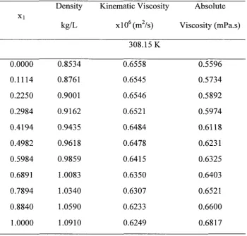
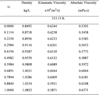
The densities and viscosities of the following quinary system: Chlorobenzene, p-xylene, octane,

ethylbenzene, and 1-hexanol and all its quaternary, ternary and binary subsystems were

experimentally measured over the entire composition range at 293.15, 298.15, 308.15, and

313.15 K.

The sets of data obtained were employed, along with other data reported in the literature, to test

the predictive capabilities of some of the most widely accepted and used models available from

the literature.

The predictive capabilities of the following models were tested: the generalized McAllister

three-body interaction model, the pseudo-binary McAllister model, the GC-UNIMOD model, the

generalized corresponding states principle (GCSP) model, the Artificial Neural Network (ANN),

and the Allan and Teja correlation.

The models testing results show that the generalized McAllister three-body interaction model

(6)

DEDICATION

This work is dedicated to my wife Amira, my sons, and to my parents for their endless love,

(7)

ACKNOWLEDGEMENTS

First and foremost, I thank Allah for endowing me health and knowledge to complete this work.

I would like to express my sincere gratitude to my advisor, Professor Abdul-Fattah A. Asfour,

and co-advisor, Dr. Ahmed Tawfik for their encouragement, guidance and for sharing their

expertise and enthusiasm with me right from the beginning of this work. I will forever be

indebted to them.

I would also like to take this chance to express my deep thanks to my wife, Amira. Without her

encouragement, support, and understanding this work would have been much harder to achieve if

not impossible. I would like also to thank my two beautiful sons, Mohamad and Ahmad for

making my life happier during the last few years.

Completing this work and obtaining this degree have been the dream of parents, making their

dream come true was always a motivation to complete this work, I just hope that this will make

them happy. My deepest appreciation and thanks also go to my sister and brothers for their

unlimited support and belief in my abilities. Also, I would like to thank all my great friends, and

classmates from school, Jordan University of Science and Technology, University of Twente,

and the University of Windsor.

Last but not least, I would like to thank all the good people in the Chemical Control Centre and

(8)

the lab more enjoyable. Special thanks are due to Bill Middleton for all the technical help he

(9)

TABLE OF CONTENTS

ABSTRACT iv DEDICATION v ACKNOWLEDGEMENTS vi

LIST OF TABLES ix LIST OF FIGURES xxiii CHAPTER 1 INTRODUCTION 1

1.1 General 1 1.2 Objectives 5 1.3 Contributions and Significance 8

CHAPTER 2 REVIEW OF THE PERTINENT LITERATURE 9

2.1 General 9 2.2 The Generalized McAllister Three-Body Interaction Model 13

2.2.1 Reaction Rate Theory 13 2.2.2 The McAllister model 17 2.2.3 Extended McAllister's model for ternary mixtures 22

2.2.4 The Asfour et al. (1991) parameters-prediction technique 23

2.2.5 Nhaesi and Asfour (1998) extended method 30 2.2.6 The generalized McAllister three-body model 30

2.3 The Pseudo-Binary McAllister Model 34 2.4 The Generalized Corresponding States Principle (GCSP) Model 36

(10)

2.5.1 Caoetal. (1992) viscosity model 41

2.5.2 "Viscosity-Thermodynamic" model (UNIMOD) 42

2.5.3 The Group Contribution (GC)-UNIMOD Model 43

2.5.4 The Nhaesi et al. (2005) parameters-prediction method 45

2.6 The Allan and Teja Correlation 46

2.7 Artificial Neural Network (ANN) 48

2.7.1 History of ANN 49

2.7.2 Network structure 51

2.7.3 Types of activation functions 52

2.7.4 Design and operation of an ANN 54

2.7.5 Application 56

2.7.6 Applications in predicting viscosity and other physical properties 58

CHAPTER 3 EXPERIMENTAL EQUIPMENT AND PROCEDURES 60

3.1 General 60

3.2 Chemicals and Purity Verification 60

3.3 Preparation of Solutions 62

3.4 Experimental Measurements 63

3.5 Density Measurement 63

3.5.1 Equipments and principle of operation 63

3.5.2 Procedures 65

3.5.3 Density Meter Calibration 66

3.6 Viscosity Measurement 66

(11)

3.6.2 Procedure 69

3.6.3 Viscometer Calibration 71

CHAPTER 4 EXPERIMENTAL RESULTS 74

4.1 Density Meter Calibration Results 74

4.2 Viscometer Calibration Results 77

4.3 The Densities and Viscosities of the Pure Components 84

4.4 Binary Systems Results 84

4.5 Ternary Systems Results 127

4.6 Quaternary Systems Results 127

4.7 Quinary Systems Results 127

CHAPTER 5 DISCUSSION 160

5.1 Testing the predictive capabilities of the generalized McAllister three-body interaction

model 161

5.2 Testing the predictive capabilities of the pseudo-binary McAllister model 169

5.3 Testing the predictive capabilities of the generalized corresponding states principle

(GCSP) model 174

5.4 Testing the predictive capabilities of the GC-UNIMOD model 182

5.5 Testing the predictive capability of the Allan and Tej a correlation 182

5.6 Testing the predictive capabilities of the ANN technique 196

5.6.1 ANN Selection and Design 196

5.6.2 ANN and Multicomponents Liquid Mixtures 197

5.6.3 ANN and the Present Multicomponents Regular Liquid Mixtures 208

(12)

CHAPTER 6 CONCLUSIONS AND RECOMMENDATIONS 238

6.1 Conclusions 238

6.2 Recommendations 239

Nomenclature 241

REFERENCES 245

APPENDIX A Excess Volume of Investigated Systems 259

APPENDIX B Raw Data of Viscosity and Density Measurements 286

APPENDIX C Estimated Experimental Error 290

(13)

LIST OF TABLES

Table 1.1: Systems Investigated in the Present Study 7

Table 3.1: Purity Verification of Pure Chemicals Used in Present Study Using Gas

Chromatography 61

Table 4.1: Calibration Data for the Density Meter 75

Table 4.2: Calculated Values of Density Meter's Constants 78

Table 4.3: Calibration Data for the Viscometer 79

Table 4.4: Pure Components Properties and their Comparison with their Corresponding

Literature Values at Different Temperatures 85

Table 4.5: Densities and Viscosities of the Binary System: Chlorobenzene (1) + p-Xylene (2)

87

Table 4.6: Densities and Viscosities of the Binary System: Chlorobenzene (1) + Octane (2) ...91

Table 4.7: Densities and Viscosities of the Binary System: Chlorobenzene (1) +Ethylbenzene

(2) 95

Table 4.8: Densities and Viscosities of the Binary System: Chlorobenzene (1) + 1-Hexanol (2)

99

Table 4.9: Densities and Viscosities of the Binary System: p-Xylene (1) + Octane (2) 103

Table 4.10: Densities and Viscosities of the Binary System: p-Xylene (1) + Ethylbenzene (2)

107

Table 4.11: Densities and Viscosities of the Binary System: p-Xylene (1) + 1-Hexanol (2) ....111

Table 4.12: Densities and Viscosities of the Binary System: Octane (1) + Ethylbenzene (2) ...115

(14)

Table 4.14: Densities and Viscosities of the Binary System: Ethylbenzene (1) + 1-Hexanol (2)

123

Table 4.15: Densities and Viscosities of the Ternary System: Chlorobenzene (1) + p-Xylene (2),

+ Octane (3) 128

Table 4.16: Densities and Viscosities of the Ternary System: Chlorobenzene (1), Octane (2), and

Ethylbenzene (3) 130

Table 4.17: Densities and Viscosities of the Ternary System: Chlorobenzene (1), p-Xylene (2),

and Ethylbenzene (3) 132

Table 4.18: Densities and Viscosities of the Ternary System: Chlorobenzene (1), Octane (2), and

1-Hexanol (3) 134

Table 4.19: Densities and Viscosities of the Ternary System: Chlorobenzene (1), Ethylbenzene

(2), and 1-Hexanol (3) 136

Table 4.20: Densities and Viscosities of the Ternary System: Chlorobenzene (1), p-Xylene (2),

and 1-Hexanol (3) 138

Table 4.21: Densities and Viscosities of the Ternary System: p-Xylene (1), Octane (2), and

Table 4.22: Densities and Viscosities of the Ternary System: p-Xylene (1) Ethylbenzene (2), and

1-Hexanol (3) 142

Table 4.23: Densities and Viscosities of the Ternary System: p-Xylene (1) Octane (2), and

1-Hexanol(3) 144

Table 4.24: Densities and Viscosities of the Ternary System: Octane (1), Ethylbenzene (2), and

(15)

Table 4.25: Densities and Viscosities of the Quaternary System: Chlorobenzene (1), p-Xylene

(2), Octane (3) and Ethylbenzene (4) 148

Table 4.26: Densities and Viscosities of the Quaternary System: p-Xylene (1), Octane (2),

Ethylbenzene (3) and l-Hexanol(4) 150

Table 4.27: Densities and Viscosities of the Quaternary System: Chlorobenzene (1), Octane (2),

Ethylbenzene (3) and 1-Hexanol (4) 152

(2), Ethylbenzene (3) and 1-Hexanol (4) 154

(2), Octane (3) and 1-Hexanol (4) 156

Table 4.30: Densities and Viscosities of the Quinary System: Chlorobenzene (1), p-Xylene (2),

Octane (3), Ethylbenzene (4) and 1-Hexanol (5) 158

Table 5.1: Physical Properties of the Pure Components Used in Kinematic Viscosity Prediction

by the Generalized McAllister Model 162

Table 5.2: Results of Testing the Generalized McAllister Three-Body Interaction Model Using

the Experimental Viscosity Data on Binary Systems 163

the Experimental Viscosity Data on Ternary Systems 165

the Experimental Viscosity Data on Quaternary and Quinary Systems 167

Table 5.5: Results of Testing the Psuedo-Binary McAllister Model Using the Experimental

(16)

Table 5.6: Results of Testing the Psuedo-Binary McAllister Model Using the Experimental

Viscosity Data on Quaternary and Quinary Systems 172

Table 5.7: Physical Properties of the Pure Components Used in Kinematic Viscosity Prediction

by the Generalized Corresponding States Principle (GCSP) Model 175

Table 5.8: Results of Testing the GCSP Model Using the Experimental Viscosity Data on Binary

Systems 176

Table 5.9: Results of Testing the GCSP Model Using the Experimental Viscosity Data on

Ternary Systems 178

Table 5.10: Results of Testing the GCSP Model Using the Experimental Viscosity Data on

Quaternary and Quinary Systems 180

Table 5.11: Number of Groups in Pure Components 183

Table 5.12: Results of Testing the GC UNIMOD Model Using the Experimental Viscosity Data

on Binary Systems 184

Table 5.13: Results of Testing the GC UNIMOD Model Using the Experimental Viscosity Data

on Ternary Systems 186

Table 5.14: Results of Testing the GC-UNIMOD Model Using the Experimental Viscosity Data

on Quaternary and Quinary Systems 188

Table 5.15: Results of Testing the Allan and Teja Model Using the Experimental Viscosity Data

on Binary Systems 190

on Ternary Systems 192

(17)

Table 5.18: The Different Combination Possibilities of the Ternary Mixtures of A, B, and C

When Modular Binary Neural Networks are Used for the Kinematic Viscosity

Prediction 199

Table 5.19: The Different Combination Possibilities of the Quaternary Mixtures of A, B, C, and

D when the Modular Binary Neural Networks are Used for Kinematic Viscosity

Prediction 202

Table 5.20: The n-Alkanes Data Used in Training and Testing the n-Alkanes Binary Network

Used for Kinematic Viscosity Prediction 205

Table 5.21: The 1-Alkanols Data Used in Training and Testing the 1-Alkanols Binary Network

Used for Kinematic Viscosity Prediction 206

Table 5.22: Summary of the Overall %AAD Values Obtained from Testing the Three Binary

Networks 207

Table 5.23: Results of Testing the ANN Technique Using the Literature Viscosity Data of

Ternary Systems (TS) of n-alkanes 209

Table 5.24: Results of Testing the ANN Technique Using the Literature Viscosity Data of the

Ternary Systems (TS) of 1 -Alkanols 210

Table 5.25: Results of Testing the Regular ANN using the Collected Experimental Viscosity

Data of the Binary Systems 216

Table 5.26: Results of Testing the Regular 1-Hexanol ANN Using the Collected Experimental

Viscosity Data of the Binary Systems 217

Table 5.27: Results of Testing the Regular Non 1-Hexanol ANN Using the Collected

(18)

Table 5.28: Results of Testing the Regular ANNs Using the Collected Experimental Viscosity

Data of the Ternary Systems 220

Data of the Quaternary System: Chlorobenzene-pXylene-Octane- Ethylbenzene

222

Data of the Quaternary System: p-Xylene + Octane +-Ethylbenzene + 1-Hexanol

223

Data of Quaternary System: Chlorobenzene + Octane + Ethylbenzene + 1-Hexanol

224

Data of Quaternary System: Chlorobenzene + pXylene + Ethylbenzene + 1-Hexanol

225

Table 5.33: Results of Testing the Regular ANNs Using the Present Experimental Viscosity Data

of Quaternary System: Chlorobenzene + p-Xylene + Octane + 1-Hexanol in Terms of

%AADofl-alkanols 226

Table 5.34: Results of Testing the Regular ANNs Using the Present Experimental Viscosity Data

on Quinary Systems in Terms of % AAD 227

Table 5.35: Overall Comparison of the Predictive Capabilities of the Tested Viscosity Model

229

Table A.l: Raw Data of Viscosity and Density Measurements for the Binary System:

(19)

Table A.2: Raw Data of Viscosity and Density Measurements for the Binary System:

Chlorobenzene (1) + Octane (2) 261

Chlorobenzene (1) +Ethylbenzene (2) 262

Chlorobenzene (1) + 1 -Hexanol (2) 263

Table A.5: Raw Data of Viscosity and Density Measurements for the Binary System: p-Xylene

(1) +Octane (2) 264

(1) + Ethylbenzene (2) 265

(1) and 1-Hexanol (2) 266

Table A. 8: Raw Data of Viscosity and Density Measurements for the Binary System: Octane (1)

+ Ethylbenzene (2) 267

Table A.9: Raw Data of Viscosity and Density Measurements for the Binary System: Octane (1)

+ 1 -Hexanol (2) 268

Table A. 10: Raw Data of Viscosity and Density Measurements for the Binary System:

Ethylbenzene (1)+1-Hexanol (2) 269

Table A.l 1: Raw Data of Viscosity and Density Measurements for the Ternary System:

Chlorobenzene (1) + p-Xylene (2), + Octane (3) 270

Table A. 12: Raw Data of Viscosity and Density Measurements for the Ternary System:

(20)

Chlorobenzene (1), p-Xylene (2), and Ethylbenzene (3) 272

Table A.14: Raw Data of Viscosity and Density Measurements for the Ternary System:

Chlorobenzene (1), Octane (2), and l-Hexanol(3) 273

Chlorobenzene (1), Ethylbenzene (2), and 1-Hexanol (3) 274

Chlorobenzene (1), p-Xylene (2), and 1-Hexanol (3) 275

Table A. 17: Raw Data of Viscosity and Density Measurements for the Ternary System: p-Xylene

(1), Octane (2), and Ethylbenzene (3) 276

(1) Ethylbenzene (2), and 1-Hexanol (3) 277

(1) Octane (2), and 1-Hexanol (3) 278

Table A.20: Raw Data of Viscosity and Density Measurements for the Ternary System: Octane

(1), Ethylbenzene (2), and 1-Hexanol (3) 279

Table A.21: Raw Data of Viscosity and Density Measurements for the Quaternary System:

Chlorobenzene (1), p-Xylene (2), Octane (3) and Ethylbenzene (4) 280

p-Xylene(l), Octane (2), Ethylbenzene (3) and 1-Hexanol (4) 281

(21)

Chlorobenzene (1), p-Xylene (2), Ethylbenzene (3) and 1-Hexanol (4) 283

Chlorobenzene (1), p-Xylene (2), Octane (3) and 1-Hexanol (4) 284

Table A.26: Raw Data of Viscosity and Density Measurements for the Quinary System:

Chlorobenzene (1), p-Xylene (2), Octane (3), Ethylbenzene (4) and 1-Hexanol (5)

285

Table B.l: The Maximum Predicted Error in the Measurement of the Kinematic Viscosity for

each Viscometer 289

Table C.l: Excess Volume of the Binary System: Chlorobenzene (1) + p-Xylene (2) 291

Table C.2: Excess Volume of the Binary System: Chlorobenzene (1) + Octane (2) 292

Table A.3: Excess Volume of the Binary System: Chlorobenzene (1) +Ethylbenzene (2) ...293

Table C.4: Excess Volume of the Binary System: Chlorobenzene (1) + 1-Hexanol (2) 294

Table C.5: Excess Volume of the Binary System: p-Xylene (1) + Octane (2) 295

Table C.6: Excess Volume of the Binary System: p-Xylene (1) + Ethylbenzene (2) 296

Table CA.7: Excess Volume of the Binary System: p-Xylene (1) and 1-Hexanol (2) 297

Table C.8: Excess Volume of the Binary System: Octane (1) + Ethylbenzene (2) 298

Table C.9: Excess Volume of the Binary System: Octane (1) + 1-Hexanol (2) 299

Table CIO: Excess Volume of the Binary System: Ethylbenzene (1) + 1-Hexanol (2) 300

Table C.l 1: Excess Volume of the Ternary System: Chlorobenzene (1) + p-Xylene (2), + Octane

(3) 301

Table C.12: Excess Volume of the Ternary System: Chlorobenzene (1), Octane (2), and

(22)

Table C.13: Excess Volume of the Ternary System: Chlorobenzene (1), p-Xylene (2), and

Table C.14: Excess Volume of the Ternary System: Chlorobenzene (1), Octane (2), and

1-Hexanol(3) 304

Table C.15: Excess Volume of the Ternary System: Chlorobenzene (1), Ethylbenzene (2), and

1-Hexanol(3) 305

Table C.16: Excess Volume of the Ternary System: Chlorobenzene (1), p-Xylene (2), and

1-Hexanol(3) 306

Table C.17: Excess Volume of the Ternary System: p-Xylene (1), Octane (2), and Ethylbenzene

(3) 307

Table C.18: Excess Volume of the Ternary System: p-Xylene (1) Ethylbenzene (2), and

1-Hexanol(3) 308

Table C.19: Excess Volume of the Ternary System: p-Xylene (1) Octane (2), and 1-Hexanol (3)

309

Table C.20: Excess Volume of the Ternary System: Octane (1), Ethylbenzene (2), and 1-Hexanol

(3) 310

Table C.21: Excess Volume of the Quaternary System: Chlorobenzene (1), p-Xylene (2), Octane

(3) and Ethylbenzene (4) 311

Table C.22: Excess Volume of the Quaternary System: p-Xylene (1), Octane (2), Ethylbenzene

Table C.23: Excess Volume of the Quaternary System: Chlorobenzene (1), Octane (2),

(23)

Table C.24: Excess Volume of the Quaternary System: Chlorobenzene (1), p-Xylene (2),

Ethylbenzene (3) and 1-Hexanol (4) 314

Table C.25: Excess Volume of the Quaternary System: Chlorobenzene (1), p-Xylene (2), Octane

Table C.26: Excess Volume of the Quinary System: Chlorobenzene (1), p-Xylene (2), Octane

(24)

LIST OF FIGURES

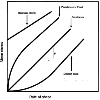
Figure 1.1: Newtonian and non-Newtonian Fluids 2

Figure 2.1: The Eyring's Model of Liquid Viscosity 15

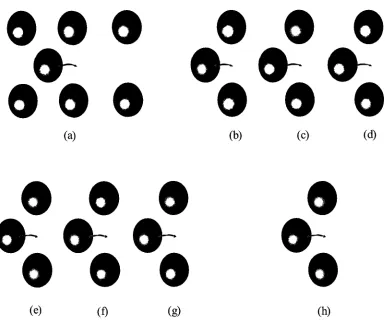
Figure 2.2: Possible Types of Interactions Among the Molecules of Binary System 19

Figure 2.3: Variation of the lumped term N12( N12 Nl)-l/3 versus the absolutr temperature

inverse [Asfour et al. (1991)] 26

Figure 2.4: Variation of the lumped term N12( N12 Nl)-l/3 versus the term

[(N2-N1)2(N12N2)-1/3] Asfour et al. (1991) 29

Figure 2.5: The representation of 2-methyl-lpropanol based on the group contribution principle

40

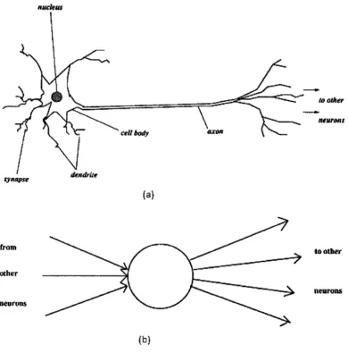
Figure 2.6: (a) Schematic diagram of real neuron (b) Schematic diagram of artificial neuron

50

Figure 2.7: A representation of an artificial neuron 53

Figure 2.8: the different types of activation functions 55

Figure 3.1: Pictorial view of the Anton-Paar density meter and the temperature controlled

chamber 68

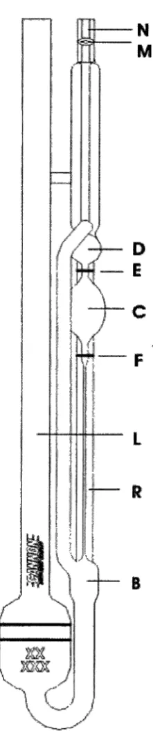
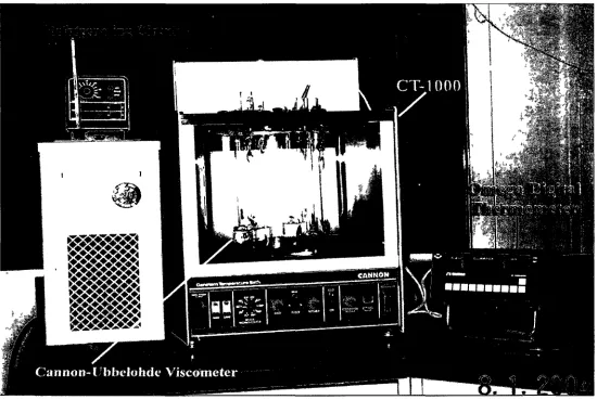
Figure 3.2: The Cannon-Ubbelohde viscometer 72

Figure 3.3: The experimental set up used for viscosity measurements 73

Figure 5.1: Predictive capabilities of the tested viscosity models for binary systems 230

Figure 5.2: Predictive capabilities of the tested viscosity models for Ternary systems 231

Figure 5.3: Predictive capabilities of the tested viscosity models for quaternary systems .... 233

Figure 5.4: Predictive capabilities of the tested viscosity models for quinary systems .... 234

(25)

CHAPTER 1

INTRODUCTION

1.1 General

Different fluids have different physical and chemical properties that determine the proper ways

to handle, store, use, process, and transport them. One of the important and common processes

encountered in real life and industrial applications is fluid transport. For these applications it is

important to know the fluid's ability to flow or in other words the fluid's resistance to flow.

Fluids in general are qualitatively described as either thin or thick fluids. Thin fluids are those

less resistant to flow and thick fluids are more resistant to flow.

A fluid in laminar flow can be viewed as if it is moving in layers. If an external shear stress is

applied to one layer of a confined fluid it will move at a certain velocity. As a result, the adjacent

layer will move at a lower velocity. This results in the development of a velocity gradient

(sometimes referred to as the rate of shear) within the fluid that is related to the shear stress. With

the help of a simple relation, Newton's law of viscosity, defines a fluid's viscosity as the

proportionality constant that relates shear stress (xxy) to the developed velocity gradient (dvx/dy).

The following equation is the mathematical representation of Newton's law of viscosity:

(26)

Fluids that obey Newton's law are designated as Newtonian fluids. Fluids for which the shear

stress is related to the velocity gradient by a more complicated relationship than Newton's law of

viscosity are known as non-Newtonian fluids and are classified on the basis of the relationship

between the shear stress and the velocity gradient. Figure 1.1 shows the different behaviours of

Newtonian and non-Newtonian fluids in terms of the relation between the shear rate (velocity

gradient) and the shear stress.

Rate of shear

(27)

Scientists and engineers use the value of the physical property of viscosity to precisely describe a

fluid's internal resistance to flow under shear stress. It is important to know a fluid's viscosity in

order to estimate the energy needed to overcome such a resistance in a flow system. Flow

systems are extensively employed in engineering applications, especially in heat exchangers as

well as in mass transfer processes.

A fluid's viscosity is a function of temperature. In the case of liquids, the viscosity decreases as

the temperature increases, whereas in the case of gases, at low density, the viscosity increases

with temperature. The difference in the temperature effect on viscosity between gases and liquids

was explained by Bird et al. 1960 as follows: "in gases (in which the molecules travel long

distances between collisions) the momentum is transported primarily by the molecules in free

flight, whereas in liquids (in which the molecules travel only very short distances between

collisions) the principal mechanism for momentum transfer is the actual colliding of the

molecules."

For the case of liquid mixtures, composition is another parameter that significantly affects the

molecular interaction within the liquid, thus, changing the fluid's resistance to flow.

In light of the above, it is clear that the impact of the previously mentioned parameters on liquid

mixtures' viscosity comes from its impact on the intra molecular forces within the fluid. Thus its

impact on the liquid structure. As a result, it is assumed that the knowledge of the dependence of

viscosity on temperature, composition, and other parameters may provide a better understanding

(28)

theory will provide a valuable tool to scientists and engineers that enables them to accurately

predict the physical properties of different liquid mixtures' combinations at different conditions

without the need to perform costly and time consuming experiments. This has motivated many

researchers to investigate the dependence of viscosity of liquid mixtures on composition. Those

efforts have resulted in developing different models which can be classified into two categories;

viz., correlative and predictive models.

The correlative models contain adjustable parameters that can be determined using

experimentally measured values of viscosity. Predictive models can predict the dependence of

viscosity on composition and would require the knowledge of some molecular parameters and/or

properties of the pure components constituting the mixture being investigated.

Amongst the viscosity models available in the literature, five widely used and accepted viscosity

models have been considered in the present study. The predictive capabilities of those models

will be tested. The models selected are: the generalized McAllister three-body interaction model,

the pseudo-binary McAllister, the GC-UNIMOD model, the generalized corresponding states

principle (GCSP) model, and the Allan and Teja correlation. The first four models are predictive

whereas the Allan Teja model is correlative. In addition, a model based on the Artificial Neural

Network (ANN) has been developed and is tested in the present study in terms of its ability to

predict the viscosity of liquid mixtures of different compositions using the viscosity values of

(29)

The previously mentioned models predict either the absolute viscosity or the kinematic viscosity.

The kinematic viscosity is related to the absolute viscosity by the following equation:

v = ^ (1.2)

P

where v = kinematic viscosity, \i = absolute viscosity, and p = density. Therefore, in order to

investigate the predictive capabilities of the above-mentioned models, the kinematic

viscosity-density or absolute viscosity-viscosity-density data must be available.

1.2 Objectives

Contrary to popular belief, reliable data on viscosities and densities of multi-component liquid

mixtures are not readily available in the literature. Although sets of data on binary systems have

been published, ternary, quaternary, and quinary systems' data are scarcely available. The

present study is part of an ongoing research program that aims at measuring and reporting data of

multi-component liquid systems at different temperature levels. The objectives of the present

study can be summarized as follows:

To measure the densities and kinematic viscosities over the entire composition range and at

293.15, 298.15, 308.15, and 313.15 K of the quinary system: chlorobenzene, p-xylene, octane,

ethylbenzene, and 1-hexanol and all its quaternary, ternary and binary sub-systems. The

(30)

Table 1.1: Systems Investigated in the Present Study

System No.

1

2

3

4

5

6

7

8

9

10

11

12

13

14

15

16

17

18

19

20

(i) Binary Systems

Chlorobenzene - p-Xylene

Chlorobenzene - Octane

Chlorobenzene - Ethylbenzene

Chlorobenzene - 1 -Hexanol

p-Xylene - Octane

p-Xylene - Ethylbenzene

p-Xylene - 1-Hexanol

Octane - Ethylbenzene

Octane - 1-Hexanol

Ethylbenzene - 1 -Hexanol

(ii) Ternary Systems

Chlorobenzene - p-Xylene - Octane

Chlorobenzene - Octane - Ethylbenzene

Chlorobenzene - p-Xylene - Ethylbenzene

Chlorobenzene - Octane - 1-Hexanol

Chlorobenzene - Ethylbenzene - 1-Hexanol

Chlorobenzene - p-Xylene - 1-Hexanol

p-Xylene - Octane - Ethylbenzene

p-Xylene - Ethylbenzene - 1-Hexanol

p-Xylene - Octane - 1 -Hexanol

(31)

Table 1.2 (Cont'd.): Systems Investigated in the Present Study

System No.

(iii) Quaternary Systems

Chlorobenzene - p-Xylene - Octane - Ethylbenzene

p-Xylene - Octane - Ethylbenzene - 1 -Hexanol

Chlorobenzene - Octane - Ethylbenzene - 1-Hexanol

Chlorobenzene - p-Xylene - Ethylbenzene - 1 -Hexanol

Chlorobenzene - p-Xylene - Octane - 1-Hexanol

(iv) Quinary Systems

(32)

2. To test the predictive capability of the various viscosity models reported in the literature

using the data reported in this study.

3. To develop an Artificial Neural Network(s) to predict the kinematic viscosities of the

different types of multi-components liquid mixtures.

4. To test the predictive capability of the developed Artificial Neural Network(s) using the

data reported in this study and data obtained from the literature.

1.3 Contributions and Significance

The present study makes a significant contribution to the literature by providing researchers,

scientists, and design engineers with reliable experimental values of the densities and viscosities

of pure compounds as well as density and viscosity composition data, over the entire

composition range, at different temperatures for the quinary system investigated and all its

quaternary, ternary, and binary sub-systems. Such data are needed for many engineering

applications that include flow systems and design of equipment.

In addition, the development of Artificial Neural Network(s) to predict the kinematic viscosities

of different types of multi-component liquid mixtures and testing their predictive capabilities in

order to provide scientists and engineers with powerful tools that enable them to predict the

dependence of viscosity on composition in multi-component liquid systems. Furthermore, the

predictive capabilities of the already existing viscosity models in the literature were critically

tested and discussed. This would enable scientists and engineers to select the best model for their

(33)

CHAPTER 2

REVIEW OF THE PERTINENT LITERATURE

2.1 General

Modeling of materials' physical properties is of great importance to scientists and engineers. It

eliminates the need to perform time consuming and costly experimental measurements to

estimate their values when needed. Predicting flow properties of pure liquids and liquid mixtures

has been a research focus for engineers from different areas.

These flow properties are needed in a host of applications that require transportation of liquids

from their place of existence to the place of need or utilization. These types of applications

include, but are not limited to, the design of heat exchange systems, mass transfer and separation

processes, and transportation of raw materials and products from one place to another. Important

applications also include mass diffusivity and thermal conductivity estimation of liquids where

flow properties are used as independent parameters. Additionally, a better understanding of

fluids' flow properties is likely to provide a better insight into the structure of liquids.

In order to overcome fluids resistance to flow, a pressure difference is typically induced to allow

the fluids to flow. Consequently, the design of pumping systems is required to induce the

pressure difference. The flow resistance is quantatively expressed in terms of viscosity. It is

important for design engineers to have a tool that enables them to accurately estimate viscosities,

when experimental values are not readily available, for the proper sizing of pumps that provide

(34)

For pure liquids, viscosity is temperature sensitive, whereas in liquid mixtures, in addition to

temperature dependence, mixture's composition affects the mixture's viscosity. Those

independent variables influence the inter-molecular interaction forces and as a result causes

changes to liquid's structure that consequently leads to changes in a mixture's viscosity.

Several researchers have examined the relationship between viscosity and the aforementioned

independent variables. Their efforts have resulted in several models that quantify such a

relationship. The general formula for those viscosity models for liquid mixtures with n

components has the following form:

l^m =f(T,x],x2,...,xn_],(i1,|^2,...,nn,C1,C2,...) (2.1)

where \xm: mixture's viscosity,

x j: the mole fraction of component i,

u i: the viscosity of pure component i, (i = 1, 2, ...., n).

Ci, C2, ...,etc. are model constants that depend on the type of investigated system.

As per the classification of Monnery et al. (1995) liquid mixtures' viscosity models are divided

into two groups. They are either empirical models or semi-theoretical models. A model is

classified as empirical if it requires fitting of experimental data to estimate the values of some

(35)

semi-theoretical models, the relations are based on the principles of popular liquid theories but the

models' constants are adjustable and evaluated using experimental data.

The latter type of models is also divided into two subgroups viz., correlative and predictive

according to the basis on which the values of the model's constants were estimated. The model is

classified as predictive if the physical properties and/or molecular parameters of the pure

components constituting the mixture are used to evaluate the model constants. Otherwise, the

model is classified as correlative if it only uses experimental data to evaluate the model

constants.

Unlike gases where theoretical models are reliably based on the kinetic theory of gases,

theoretical description of liquids (and dense gases) is much more complicated. This is due to the

nature of the intermolecular forces, which consist of the short range (repulsion and hydrogen

bonding), wide range (electrostatic), and long range (attraction) effects [Mehrotra et al. 1996].

However, there have been several attempts to develop theoretical models for pure liquids' and

mixtures' viscosity. The main theoretical frameworks used in developing such models are either

the reaction rate theory, group contribution concept, or the corresponding states principle.

The present work is a continuation of an experimental research program at our laboratory that

aims at providing reliable experimental values of viscosity-composition and density-composition

data of pure liquids and mixtures of different types of liquids. Additionally, the measured values

are used to test the predictive capabilities of different selected empirical and semi-theoretical

(36)

The experimental viscosity data collected in the present study have been employed in testing the

predictive capabilities of the following models:

1. The generalized McAllister three-body interaction model (Nhaesi and Asfour 2000a).

2. The pseudo-binary McAllister model based on the reaction rate theory (Nhasei and

Asfour 2000b).

3. The GC-UNIMOD model, based on group contribution theory (Cao et al. 1993b).

4. The generalized corresponding states model (GCSP) model, based on corresponding

states principle (Teja and Rice 1981).

5. The Allan and Teja correlation (Allan and Teja 1991).

In addition to these models, the present study investigates the use of the artificial neural network

(ANN), which has attracted the attention of several researchers, in predicting the mixture

viscosity. The main difference between the work reported herein and the earlier work reported by

other investigators is that in the present work, the network was trained by using some of the data

on binary systems, then the trained network was employed to predict the viscosities of the

multi-component systems.

Other investigators employed some of their data to train the network then used the train network

to predict the viscosities of the same type of system; i.e., part of the binary system data were used

to train the network and the rest of the binary data were used in testing the network for binary

(37)

The first four models and the model based on the artificial neural network are predictive

semi-theoretical models, whereas the Allan Teja model is classified as a correlative model. A detailed

description of the foregoing models, their respective theoretical framework, and their

development are now in order.

2.2 The Generalized McAllister Three-Body Interaction Model

McAllister (1960) reported a model based on the reaction rate theory. McAllister's model started

as a correlative model for binary mixtures. Asfour et al. (1991) could successfully transform the

model from a correlative equation to a predictive model for the case of binary n-alkanes liquid

systems. Nhaesi and Asfour (2000a) developed and reported a generalized form of the

McAllister model which could be used for multi-component regular and w-alkane liquid

solutions. The following section reviews the theoretical basis of the original McAllister model

and the development of the generalized predictive version of the model.

2.2.1 Reaction rate theory and Eyring's equation of viscosity

The reaction rate theory is applied to liquids as suggested by Eyring (1936) and Ewell and

Eyring (1937) to describe the viscous flow of liquids. It visualizes the liquid as a group of

adjacent molecules in equilibrium positions with "dissolved" holes or vacant sites between them.

Each molecule is bonded to other molecules by different types of bonds. The total energy of

bonding is the resultant of the different bonding forces between the molecule and other

neighbouring molecules. Molecules that are able to break the bonds can jump into the dissolved

(38)

Figure 2.1a shows a schematic representation of the fluid layers as visualized by Eyring and

coworkers. It is assumed that the fluid layers are separated by a distance A,i and that the average

area available per molecule is A/2X3.

When applied to liquids, the reaction rate theory deals with viscous flow in the same fashion as a

chemical reaction. In their analogy, Eyring assumed that under shear stress, the movement of a

single molecule in one layer of the liquid requires the availability of a vacant site. The molecule

must also have sufficient energy to cross a potential energy barrier A*Go (Figure 2.1b) and

complete the "jump" from one equilibrium position to another neighbouring vacant site,

"dissolved hole". This move is analogous to an elementary step in chemical reactions.

Molecular motion can occur in both directions, forward and backward. For static liquids without

any external force acting on the liquid, molecular movement (or jumping) is caused by thermal

activation at the same rate in opposite directions and does not result in a net flow. Consider a

liquid where a shear force, f, is applied to the liquid in the forward direction, the mechanical

work done by the force is used to provide the molecules with sufficient energy to rise above the

energy barrier. This mechanical work is equal to fA-2^-3 (A/2) and is used to bring the molecule to

the top of the peak. Then, the gained energy is given off as heat by the traveling molecule as it

(39)

I

. 3 1 —

$

(4

(b)

(40)

As a result of the work done by the shear force, the energy barrier decreases for the forward

jumping by the value of the performed work. On the contrary, it increases by the same magnitude

for the backward jumping. Consequently, a net flow in the forward direction occurs.

The final form of the viscosity equation suggested by Eyring is:

\x = ^ exp( 2.) (2.2)

A^A/jA k l

where k is Boltzman constant and h is Plank's constant.

Two assumptions are made. The first one is that \~%i and the second one is that the term X\ X2 X?,

represents the average volume per molecule, or the effective volume of the molecule, Vo, which

is given by the following equation:

V0= Vm/ N

(2.3)

where Vm is the molar volume and N is Avogadro's number.

Therefore, combining the last two assumptions with the previous equation gives the following

formula:

(41)

where A*G is the activation energy of viscous flow per mole, and R is the universal gas constant.

Equation (2.4) is known as Eyring's equation of viscosity. There is another form of the same

equation that is written in terms of the kinematic viscosity. That form is written as

v = exp( ) (2.5) M RT

where M is the molecular weight.

2.2.2 The McAllister model

McAllister (1960) developed a model for the calculation of the dependence of viscosity on

composition of liquid binary mixtures. The model is based on Eyring's reaction rate theory.

McAllister (1960) used Eyring's viscosity equation (equation 2.5) to develop a new viscosity

model for binary liquid mixtures of two components viz., type 1 and type 2. For such a mixture,

if a molecule of type 1 jumps to a neighbouring vacant site by crossing an energy barrier, it may

interact with molecules of type 1 or 2 or both depending on the local concentrations of

neighbouring components' type.

According to McAllister, this interaction is assumed to be a three-body interaction. McAllister

stated that this assumption is valid for the cases where the difference in the molecular sizes of the

two types of molecules is relatively small. He suggested that the molecular diameter ratio must

be less than 1.5 for this assumption to be valid. For molecules with a higher diameter ratio, a

(42)

For the three-body interaction assumption, there are six possible types of interactions. These

types are: 1-1-1, 2-2-2, 1-2-1, 2-1-2, 1-1-2, and 1-2-2. Figure 2.2 depicts the different types of

interaction.

McAllister made the following major assumptions when developing his model for binary

mixtures:

The activation free energies of viscous flow are assumed to be additive quantities.

The probability of occurrence of different types of interactions is only proportional to the mole

fractions of the mixture's components.

Therefore, the activation free energy of the mixture, A*G, is given by;

A

*

G

= Z Zi>

l X j

x

k

**A*G**

1 J k

(2.6)

,=i J =i k=i

where x„ x,, Xk are the mole fractions of the components constituting the mixture.

In addition, the following assumptions were made to simplify the relationship and reduce the

number of unknowns in equation (2.6):

(43)

9 9 9 9 9 9

9 9 9~ 9~

9 9 9 9 9 9

(a) (b) (c) (d)

9 9 9

9^ 9~ 9r

9 9 9

9 ^P~*

9

(e) (f) (g) (h)

(44)

A * G2 I 2= A * G1 2 2= A * G2 1 (2.8)

Substituting equations (2.7) and (2.8) into the expanded form of equation (2.6) yields,

A*G = x^A*G1 + 3x12x2A*G12 + 3x,x21A*G21 +x32A*G2 (2.9)

For a binary mixture, equation (2.4) is written in terms of kinematic viscosity, v, as follows:

v =

i^

e x p (

^)

( 2

.

1 0

)

M„ RT

where Mm is the molecular weight of the mixture. For a binary mixture Mm is assumed to be

equal to (xiMi+x2M2).

Substituting for A*G from equation (2.9) into equation (2.10); one gets

hN ,x?A*G,+3x?x,A*G1 2+3x,x2 !A*G2 1+x2 iA*G2 N / 0 1 1,

v = exp(—! —- — - - ) (2.11)

M„ RT m

(45)

hN AG

v i = exp( 4 (2.12)

1 M, RT V '

and for pure components of type 2

hN i G 2,

v2 = e xP(——) (2.13)

2 M, RT V ;

For interaction of type 1-2

hN ,A*G12,

**' • ' - ^ r " * - ^**

(114)

where Mi2 is given by

Mn= l- 2- (2.15)

whereas, for interaction of type 21

v.-|W^>

(46)

2 M , + M ,

M2, = 2- L (2.17)

Taking the natural logarithms of equations (2.10) through (2.16) and rearranging, one obtains

equation (2.18) which represents the final and common form of the McAllister three-body

interaction model.

Inv = x^nv, +3x2lxjnvn +3xjX2^nv21 + x\inv2

- M x , +x2M2 /M,) + 3x?x2fa(2 + M 3 2 / M l) ( 2 > 1 8 )

+3x

lX

^n(

1 + 2 M 2 / M l

) + x

3

XM

2

/M,)

where vn and V21 are adjustable parameters which can be determined using experimental

kinematic viscosity-composition data.

This model is considered one of the best correlative techniques for the viscosity of binary liquid

mixtures (Reid et al. 1987).

2.2.3 Extended McAllister's model for ternary liquid mixtures

As stated earlier, McAllister's three-body model is applicable for binary liquid mixtures. Three

years after the work of McAllister was published, Chandramouli and Laddha (1963) developed

and reported a new version of McAllister's three-body model that can be used for ternary liquid

(47)

In addition to the binary interaction parameters, ternary interaction parameters were introduced.

The final form of the extended McAllister's three-body model is given by the following

equation:

£nv = xjVnVj +x2£nv2 + x3^nv3 +3xfx2^nv12 +3xfx3^nv13

+ 3x2x/nv2 1 +3x2x3^nv2 3 +3x3x,^nv3 1 +3x3x2£nv3 2

+ 6x1x2x3^nv123 - . f t i ^ M j + x2M2 + x3M3) + xf^nMj

+ x ^ n M2 + x3^ n M3 + 3 x f x2l n (2 M' +Ml )

„ 2 n 2 M , + M3 x „ 2 a , 2 M2+ M . N

+ 3xf x3£n( l- - ) + 3 x2x / n ( - L)

, n 2M2+1VL „ 2 , 2 M , + M , N

+ 3 x2x A ( 1_ L) + 3 x2x / n ( 3_ L )

„ 2 . . 2 M3+ M2. . . , M , + M2+ M3.

+ 3x3x2£n( 3- 2-) + 6x1x2x3^n(—l- 2- 3-)

(2.19)

where: V12, V21, V13, V31, V23, and V32 are binary interaction parameters, and V123 is the ternary

interaction parameter.

The values of the binary and ternary interaction parameters are determined by fitting

(48)

2.2.4 The Asfour et al. (1991) parameter- prediction method

As indicated earlier herein, Reid et al. (1987) considered the McAllister model to be one of the

best correlative techniques for the viscosity of binary liquid mixtures. But being correlative is a

significant disadvantage of this model. Its correlative nature calls for the need to carry out both

time consuming and costly experiments in order to estimate the values of the adjustable

parameters.

This major drawback was overcome by Asfour and co-workers. They were able to develop a

technique that converts the McAllister model from a correlative model into a predictive model.

Asfour et al. (1991) introduced a modification to the McAllister model that uses the molecular

parameters and the viscosities of pure components to predict the values of the interaction

parameters in McAllister's model for binary n-alkane liquid mixtures.

For the n-alkane liquid mixtures, Asfour et al. (1991) started with the assumption that the binary

interaction parameters in the McAllister model, v n and V21, are related to the mixture's pure

components kinematic viscosities as follows:

v1 2o c (V l 2v2), / 3 (2.20)

(49)

Dividing equation (2.20) by equation (2.21) results in the following relationship between the two

adjustable parameters:

V2 1 =V1 2

(

v

/ 3

12. (2.22)

In addition to that, Asfour et al. (1991) plotted the lumped term vn( vi2 V2)"1/3 versus the inverse

of the absolute temperature using data of several n-alkane binary mixtures. Those mixtures are:

hexane heptane, hexane octane, heptane octane, heptane decane, tetradecane

-hexadecane, and octane - decane. The experimental data were taken from Cooper (1988). They

were selected to satisfy the condition of having the differences in number of carbon numbers to

be less than or equal to 3. They assumed that this condition justify the use of McAllister

three-body interaction model.

The resulting plot showed a straight line with a slope of zero as shown in Figure 2.3. This has led

(50)

i - l

l . U O

1.04

1.02

i nn

m

— •

•——

n

"

•

D

•*

?

•

O

•

A

0

1

•

- — ^ ^ s >

D

•

6

1

3.15 325 335

(1/T)xl0* K

1

3.45

-1/3-Figure 2.3: Variation of the Lumped Term vi2( vi2 Vi)" Versus the Absolute

Temperature Inverse [Asfour et al. (1991)].

A Hexane (A) - Heptane (B)

o Heptane (A) - Octane (B)

• Tetradecane (A) - Hexadecane (B)

0 Hexane (A) - Octane (B)

• Heptane (A) - Decane (B)

(51)

Moreover, Asfour et al. (1991) plotted the lumped term V12 ( Vi2 vi)"1/3 that was proven to be

temperature independent verses another lumped term [(N2-Ni)2/(Ni2N2)1/3], where the Ni and

N2 are the number of carbon atoms per molecule of components 1 and 2, respectively.

Components 1 and 2 constitute the liquid mixture. They used experimental data of the same

n-alkane binary mixtures they previously used to make the plot shown in Figure 2.3.

The plot as shown in Figure 2.4 resulted in a straight line with a slope that suggests a linear

relationship between the two lumped terms. Using the least-squares technique, Asfour et al.

(1991) obtained the following equation:

Vl2 - 1 + 0.044 (^2 2 ™l£ (2.23)

(v2v2), / 3 (N?N2y

Therefore, with the help of equation (2.22) and (2.23) the values of the adjustable parameters V12,

and V21 in the McAllister model could be estimated using only the physical properties of the

pure components constituting the liquid mixture. The significance of this work is in transforming

the McAllister three-body interaction model from a correlative to a predictive model and

consequently extending its usefulness and practicality.

As stated earlier, the Asfour et al. (1991) work was based on McAllister three-body interaction

model that is assumed to be applicable where the differences in carbon numbers of the

components composing the mixture are less than or equal 3. For other n-alkane binary liquid

(52)

1.06

9

1,04

1.02

LOO

0,00

<N2-Ni)2(Ni2N2)"l/3

1.20

1/3

Figure 2.4: Variation of the Lumped Term vi2( vi vi)" Versus the Term

[(N2-Ni)2(Ni2N2)"1/3]. Asfour et al. (1991).

A Hexane (A) - Heptane (B)

o Heptane (A) - Octane (B)

• Tetradecane (A) - Hexadecane (B)

0 Hexane (A) - Octane (B)

• Heptane (A) - Decane (B)

(53)

developed another equation that is based on the McAllister four-body interaction model. They

suggested the following equation for calculating the quaternary interaction adjustable parameter,

1122 _ i ,_{= 1 + 0 0 3 ^} n m ^ ' 2 _N]>)_{(2 24)}

Furthermore, Asfour et al. (1991) suggested two equations to calculate the other quaternary

interaction adjustable parameters, vuu andv1222, in terms of the first parameter, v]122, estimated

from equation (2.24). The two equations are as follow:

V1112 — V1 1 2 2

V2 2 2 1 ~~ V1 1 2 2

( V/4 12. vv. y

( V/4 v2

vvi y

(2.25)

(2.26)

In spite of the good improvement that Asfour et al. (1991) have brought to the McAllister model,

their technique was only applicable to binary liquid n-alkanes mixtures. In subsequent work,

Nhaesi and Asfour (1998) used a similar approach to extend the technique to binary regular

liquid mixtures. They introduced a different definition than that introduced earlier by Allan and

Teja (1991) for the effective carbon number, which made it much easier and much less

cumbersome to calculate and apply. This enabled Nahesi and Asfour (1998) to estimate the

effective carbon number (ECN) for regular liquid components from the value of the kinematic

viscosity of the component at 308.15 K. They suggested the following relationship:

(54)

where A= - 1.943 and B = 0.193, and [email protected] is the kinematic viscosity, in cSt, of the pure

regular component at 308.15 K.

The value of the kinematic viscosity at 308.15 K is substituted into equation (2.27) in order to

obtain the ECN of the compound of interest.

2.2.5 Nhaesi and Asfour (1998) extended method

Nhaesi and Asfour (1998) introduced an equation analogous to that developed for n-alkanes for

predicting the binary interaction parameters for regular mixtures using the ECN instead of the

number of carbon atoms in the case of n-alkanes. The new equation is given by,

2V'2 ... = 0.8735 + 0.0715 ( E C N z 2 E C N») 3 (2.28) (v,2v2)1/3 (ECN2ECN2)1/3

Equation (2.22) is used to predict the value of V21.

2.2.6 The generalized McAllister three-body model

The next major improvement to the McAllister three-body interaction model was introduced by

Nhaesi and Asfour (2000a). They developed a new generalized technique to predict the

(55)

In developing their model they started with the assumption that the free activation energies for

viscous flow are additive. Therefore, the free activation energy of the mixture, AGm, is given by

AGm = J>?AG, +3± Jx,2xJAG1J +6XZI>1xJxkAG1 J k (2.29)

1=1 1=1 j = l 1=1 j = l k = l

where n is the number of components constituting the mixture.

In addition, they assumed that the activation energies depend only on the type of components

involved not their order. They proposed the following equations:

AGy,= AGUJ= AGy

AGJIJ=AG1JJ=AGJ1

The starting point of the model is McAllister's viscosity equation that is written for a liquid

mixture as,

hN AG

v , = — e x p ( :-) (2.30)

1 M, RT

vm = exp( —) (2.31)

(56)

where k is Boltzman constant, h is Plank's constant, R is the universal gas constant, and

N is Avogadro's number.

The subscript m in equation (2.31) refers to the mixture and the subscript i refers to pure

component i. vm is the kinematic viscosity of the mixture, M is the molecular weight. The

average molecular weight of the mixture, Mm, is calculated using the following mixing rule:

Mm=2;x1MI (2.32)

where M, is the molecular weight of pure component i.

For a binary interaction of type ij

hN AG,,

v =—-exp(—-2.) (2.33) •I = C AR

1J My RT

where M,j is

2 M , + M ,

M„= '- i- (2.34)

(57)

hN A Gk

v„k = e xP ( —) (2.35)

J M1Jk RT V '

where Myk is

M , + M . + M ,

Ml j k= — f—± (2.36)

By incorporating equations (2.30) through (2.35) into equation (2.29) one obtains,

n o n n 2

! n vm= X xfln(v.M.) + 3 I E xfx/n(v..M..)

m • 1 i * i • i • 1 ! j y y"

i = i 1 = 1 j = i J J J

n n n (2.37)

i * j * k

The number of binary interaction parameters, N2, and ternary interaction parameters, N3 in

equation (2.37) are calculated using the following two equations:

n!

N, = (2.38) 2!(n-2)!

n!

N3 = (2.39)

3 3!(n-3)!

The concept of effective carbon number (ECN) is employed for the pure regular liquid

components. Nhaesi and Asfour (1998) suggested the use of equation (2.27) to determine the

numerical value of the effective carbon number of regular liquid components and equation (2.28)

for predicting the values of the adjustable parameters of type ij. The values of the other binary

(58)

interaction parameters, Nhaesi and Asfour (2000a) developed the following equation to predict

the ternary interaction parameters for n-alkanes:

v K (N - N ">

•JK _ n nn/i 1 i n m i / ; ' 7v k x ,i / 2

= 0.9941 + 0.03167^-^ ^ - (2.40)

2.3 The Psg«rfo-Binarv McAllister Model

The second model that will be tested in this study is the pseudo-binary McAllister model. This

modification utilizes the pseudo-binary concept that was introduced by Wu and Asfour (1992)

with the generalized McAllister model reported by Nhaesi and Asfour (2000).

In the "pseudo-binary" model, a multi-component liquid mixture of n components is treated as a

binary mixture of component 1 and a "pseudo-component" that represents the remaining

components of the mixture (2, 3, 4,.., n). The reduction of the number of components in

multi-component liquid mixture to two multi-components significantly reduces the complexity of

calculations and leads to dramatic reduction in calculation time by requiring fewer calculation

steps.

Wu and Asfour (1992) introduced the pseudo-binary concept and utilized it in modifying the

generalized corresponding states principle (GCSP), which will be discussed later in this chapter.

Nhaesi and Asfour (2000b) incorporated the pseudo-binary model into the generalized

McAllister three-body interaction model which led to the development of the pseudo-binary

McAllister model for predicting the viscosities of n-alkane liquid mixtures.

In addition, they used the effective carbon number, ECN, concept explained earlier to extend the

(59)

regular liquid mixtures. For the regular pure components, the ECN is calculated using equation

(2.27). For the "pseudo-component, Nhaesi and Asfour (2000a) suggested the use of the

following mixing rule to determine its ECN in terms of the those for the pure components

constituting the "pseudo-component:

(ECN^^XXECN), (2.41)

i=2

The kinematic viscosity of the "pseudo-component is calculated with the help of the following

equation:

lnv2. =fjXl(£nv1) (2.42)

1=2

The molecular weight of the "pseudo-component is calculated using the following equation:

^nM

2

.=5]X

I

(^nM

I

) (2.43)

1=2

The term Xj in equations (2.41) through (2.43) represents the normalized mole-fraction of

component i in the "pseudo-component. This quantity is calculated using the following

(60)

X , = V - (2-44)

i=2

For regular mixtures, the numerical values of (ECN)i, Mi, and vi for the "pseudo-component

obtained from equations (2.41) through (2.43) are substituted into equations (2.28) and (2.22) for

regular mixtures in order to predict the McAllister's binary interaction parameters, V\i and vn.

The same procedure is followed when using this technique for n-alkanes but the components'

carbon numbers are used instead of the ECN in the calculations.

2.4 The Generalized Corresponding States Principle (GCSP) Model

The third model that will be tested in this study is the Generalized Corresponding States

Principle (GCSP) viscosity model. The original corresponding states principle (CSP) is based on

the reduction of variables by using critical properties; e.g., critical pressure, volume and

temperature to calculate a new dimensionless reduced parameters. The reduced parameters

represent the ratios of the independent variable to the corresponding critical condition.

The corresponding states principle is based on the assumption that different fluids at the same

reduced conditions of temperature, pressure, and/or volume have the same reduced physical

properties.

Taj a and Rice (1981) utilized the corresponding states principle and used it to develop a new

(61)

generalized corresponding states principle (GCSP). Their model was based on the liquid's

critical volume.

In 1986, Taj a and Thurner suggested another form of the Taj a and Rice model in that it is based

on the critical pressure to avoid the effect of the relatively high experimental uncertainties

commonly associated with the measurement of critical volumes and suggested the use of the

following equation for viscosity prediction:

M l ^ ) = Mn£>

rl

+ J

2

_

(

° J

r l

[ ^ ( ^ )

r 2

- ^ ( ^ )

r l

] (2.45)

where rl and r2 refer to two non-spherical fluids, \i is the absolute viscosity, co is the acentric

factor of the non-spherical fluid, and ^ is an adjustable parameter obtained from the critical

properties of the fluid and is given by the following equation:

y _ p - 2 / 3Tl / 6M- l / 2

S-^c 1c M (2.46)

where Pc, Tc , and M in equation (2.46) are the critical pressure, temperature, and molecular

weight, respectively.

In order to apply equation (2.45) to liquid mixtures, Taja and Thurner (1986) recommended the

use of a group of mixing rules that were suggested earlier by Wong et al. (1984) to determine the

pseudo-critical properties and parameters of the liquid mixture. Wong et al. (1984) mixing rules

Study of the Viscometric and Volumetric Properties of Multicomponent Regular Liquid Systems at Different Temperature Levels

Scholarship at UWindsor

Scholarship at UWindsor

Study of the Viscometric and Volumetric Properties of

Study of the Viscometric and Volumetric Properties of

Multicomponent Regular Liquid Systems at Different Temperature

Multicomponent Regular Liquid Systems at Different Temperature

Levels

Levels

Multicomponent Regular Liquid Systems at Different Temperature

Levels

By

Nidal Hussein

Windsor, Ontario, Canada

2012

1*1

ABSTRACT

LIST OF TABLES

LIST OF FIGURES

Rate of shear

(4

*

= Z Zi>

x

A*G

(2.6)

9 9 9 9 9 9

9~~ 9~~ 9~ 9~

9 9 9 9 9 9

9 9 9

9^ 9~ 9r

9 9 9

9

^P~*

9

i^

^)

.

)

' • ' - ^ r " * - ^

v.-|W^>

+3x

^n(

) + x

XM

/M,)

(

v

— •

•——

•*

?

•

1

•

(1/T)xl0* K

9

^nM

.=5]X

(^nM

) (2.43)

M l ^ ) = Mn£>

+ J

_

° J

[ ^ ( ^ )

- ^ ( ^ )

] (2.45)

**1*1**

**A*G**

9 9 9~ 9~

**' • ' - ^ r " * - ^**