Evaluation of Computational Fluid Dynamics (CFD) for Modeling UV-Initiated Advanced Oxidation Processes

ABSTRACT

ALPERT, SCOTT MICHAEL. Evaluation of Computational Fluid Dynamics (CFD) for Modeling UV-Initiated Advanced Oxidation Processes. (Under the direction of Joel J. Ducoste.)

The use of ultraviolet-initiated (UV-initiated) advanced oxidation processes (AOP) is rapidly becoming an attractive alternative for the degradation of emerging organic contaminants that are not easily removed using conventional water treatment processes. Design and optimization of UV/H2O2 systems must incorporate both reactor design

(hydrodynamics, lamp orientation) and chemical kinetics (reaction mechanisms, kinetic rate constants). This research lays the groundwork for a protocol for using CFD models to simulate UV-initiated AOPs and, in doing so, provides the start for an improved design process to meet the needs of the water treatment community. In this CFD model, the combination of turbulence sub-models, fluence rate sub-models, and kinetic rate equations results in a comprehensive and flexible design tool for predicting the effluent chemical composition from a UV-initiated AOP reactor.

To validate the CFD simulation, the results of the model under various operating conditions were compared to pilot reactor trials conducted with the target contaminants methylene blue and the antimicrobial compound sulfamethoxazole. Using the standard k-ε

measured in the pilot reactors. Additional investigation into the hydrodynamic effects and the light model validation is recommended to determine the next steps for model revision to improve agreement with experimental results.

Evaluation of Computational Fluid Dynamics (CFD) for Modeling UV-Initiated Advanced Oxidation Processes

by

Scott Michael Alpert

A dissertation submitted to the Graduate Faculty of North Carolina State University

in partial fulfillment of the requirements for the Degree of

Doctor of Philosophy

Civil Engineering

Raleigh, North Carolina 2008

APPROVED BY:

DEDICATION

To Shannon, With Love.

BIOGRAPHY

ACKNOWLEDGEMENTS

I would like to acknowledge and thank all of the people who have helped and supported me in the completion of this degree:

My friends at NC State, especially Tarek Aziz, Erin Gallimore, and Colleen Bowker, all of whom always listened and offered support.

The students and friends who helped with the research, including Olivier Prat, Carolina Baeza, Alfred Rossner, Colleen Bowker, Xi Zhao, Kiseok Jang, Matt Strickland, and Catherine Hoffmann.

My dissertation committee who provided great insight into the topic: Joel Ducoste, Detlef Knappe, Karl Linden, and David Ollis.

My funding sources: American Water Works Association Research Foundation, including our project manager Alice Fulmer and the Project Advisory Committee; and the Preparing the Professoriate Program at NC State.

All of my colleagues at HDR Engineering, Inc. who remained flexible during these 6+ long years.

My good friends in Raleigh: Jennifer, Ben, and Claire Heard.

My Mom Faye Alpert for her support and all of the great conversations on the drive to and from Raleigh.

My In-laws Skip and Vicki Atkinson for all their words of wisdom.

TABLE OF CONTENTS

LIST OF TABLES………...………..…viii

LIST OF FIGURES………...x

1. INTRODUCTION ... 1

1.1 Originality and Relevance ... 2

1.2 Hypotheses... 3

2. LITERATURE REVIEW ... 5

2.1 Ultraviolet Photochemistry ... 5

2.2 Advanced Oxidation ... 10

2.3 Computational Fluid Dynamics ... 13

2.4 Turbulence Models ... 16

2.5 Mixing Models... 21

2.6 Fluence Rate Models ... 25

2.7 Chemical Contaminants... 31

2.7.1 Dye Decolorization ... 32

2.7.2 Sulfamethoxazole Oxidation... 47

2.8 Advanced Oxidation Process Optimization... 53

3. RESEARCH APPROACH AND METHODS ... 58

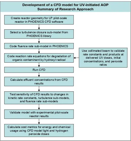
3.1 Development of a CFD Model for UV-initiated Advanced Oxidation ... 58

3.3.2 Analytical Methods... 66

3.3.2.1 Methylene Blue Calibration Curve ... 70

3.3.2.1 Sulfamethoxazole Calibration Curve... 71

3.4 Collimated Beam Testing of Dye Degradation... 72

3.4.1 Kinetic Rate Constants... 76

3.4.2 Dye Degradation Reaction Reversibility and Stability... 80

3.5 CFD Evaluation of Turbulence and Fluence-Rate Sub-Models ... 81

3.6 CFD Model Evaluation of Design Parameters ... 82

3.7 Validation of CFD Results for Dye Degradation Using the Pilot-Scale Reactor ... 83

3.7.1 Impact of Internal Baffle Configuration on UV/AOP Performance... 89

3.8 Advanced Oxidation of Sulfamethoxazole ... 89

3.9 Optimization of Energy and Hydrogen Peroxide Usage ... 90

3.10 Other Numerical Methods ... 91

4. RESEARCH RESULTS AND DISCUSSION ... 98

4.1 Experimental Results – Collimated Beam Apparatus... 98

4.1.1 Second-Order Kinetic Rate Constant for Methylene Blue and the Hydroxyl Radical ... 98

4.1.2 Effects of the Molar Ratio of Hydrogen Peroxide to Methylene Blue ... 101

4.1.3 Stability and Reversibility of the Methylene Blue Degradation Reaction... 104

4.2 Experimental Results – Pilot Reactor ... 108

4.2.1 Methylene Blue... 110

4.3 Computational Fluid Dynamics ... 120

4.3.1 Grid Independence ... 120

4.3.2 Comparison of Experimental Results to CFD Model Results ... 121

4.3.2.1 Methylene Blue... 123

4.3.2.2 Sulfamethoxazole... 131

4.3.4 Fluence Rate Sub-model Analysis ... 136

4.3.5 Second-Order Kinetic Rate Constant Analysis... 140

4.3.6 Turbulence Sub-model Analysis... 141

4.3.7 Radical Scavenger Analysis... 145

4.3.8 Micromixing ... 148

4.3.9 Cost Metrics ... 149

4.4 Other Numerical Methods ... 154

4.4.1 Reaction Mechanism Equations... 154

4.4.2 Dose Distributions ... 155

4.5 Future Research Opportunities ... 163

5. JOURNAL ARTICLE NUMBER 1 ... 166

6. JOURNAL ARTICLE NUMBER 2 ... 205

7. LIST OF REFERENCES... 258

8. APPENDIX... 270

8.1 Appendix A – Sample CFD Codes for Pressure/Velocity, Light, and Kinetics ... 271

LIST OF TABLES

Table 2.1: Variables in Turbulence Closure Sub-models ... 20

Table 2.2: Properties of Several Organic Dyes... 33

Table 2.3: Characteristics of Sulfamethoxazole ... 49

Table 2.4: pH Dependent Kinetic Rate Parameters (Canonica et al., 2008)... 51

Table 3.1: CFD Model Boundary Conditions... 60

Table 3.2: Variables in CFD Codes ... 64

Table 3.3: Constants in CFD Codes... 65

Table 4.1: Experimental Values for the Methylene Blue Kinetic Rate Constant ... 99

Table 4.2: Methylene Blue Stability Results ... 107

Table 4.3: Research Conditions Evaluated with Pilot Scale Reactor ... 110

Table 4.4: Pilot Results for Research Condition No. 1... 111

Table 4.5: Pilot Results for Research Condition No. 2... 111

Table 4.6: Pilot Results for Research Condition No. 3... 112

Table 4.7: Pilot Results for Research Condition No. 4... 112

Table 4.8: Pilot Results for Research Condition No. 5... 113

Table 4.9: Pilot Results for Research Condition No. 6... 113

Table 4.10: Pilot Results for Research Condition No. 29... 114

Table 4.11: Pilot Results for Research Condition No. 30... 114

Table 4.12: Pilot Results for Research Condition No. 35... 115

Table 4.13: Pilot Results for Research Condition No. 10a (SMX Direct Photolysis) ... 118

Table 4.14: Pilot Results for Research Condition No. 10b (SMX AOP & Direct Photolysis) ... 119

Table 4.15: Grid Independence Data ... 121

Table 4.16: Research Condition No. 1... 123

Table 4.17: Research Condition No. 2... 124

Table 4.18: Research Condition No. 3... 124

Table 4.19: Research Condition No. 4... 125

Table 4.20: Research Condition No. 5... 125

Table 4.21: Research Condition No. 6... 126

Table 4.22: Research Condition No. 29... 126

Table 4.23: Research Condition No. 30... 127

Table 4.24: Research Condition No. 35... 127

Table 4.25: Research Condition No. 10a – Direct Photolysis of SMX ... 132

Table 4.26: Research Condition No. 10b – SMX Advanced Oxidation and Photolysis ... 133

Table 4.27: Impact of Fluence Rate Model on CFD Results... 139

Table 4.28: Impact of Second-Order Rate Constant kMB,•OH on CFD Results... 140

Table 4.29: Impact of Turbulence Sub-model on CFD Results... 145

Table 4.31: Annual Average Cost per Order for Research Conditions ... 150

Table 4.32: Summary of Numerical Solution Results ... 159

Table 4.33: Example of Model Effect on Regulatory Requirements... 161

LIST OF FIGURES

Figure 2.1: Relationship Among Incident, Refracted, and Reflected Light ... 9

Figure 2.2: Angle Geometry of Attenuation Factor in RAD-LSI Model ... 28

Figure 2.3: Geometry of Focus Factor in MSSS Model ... 31

Figure 2.4: Protonation States of Sulfamethoxazole (based on Boreen et al., 2004) ... 49

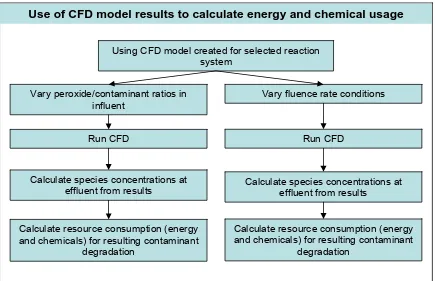
Figure 3.1: Chart Summary of Research Approach... 59

Figure 3.2: Reactor Geometry within PHOENICS... 61

Figure 3.3: CFD Grid Spacing in Y-Z Plane ... 62

Figure 3.4: CFD Grid Spacing in X-Z Plane ... 62

Figure 3.5: CFD Grid Among Internal Baffles and Wiper Mechanism ... 62

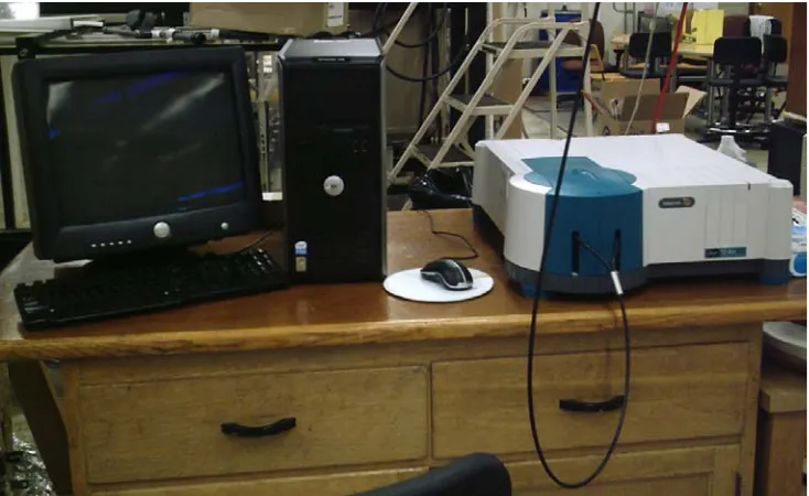
Figure 3.6: Photograph of Pilot Reactor Spectrophotometer System ... 67

Figure 3.7: Spectrophotometric Probe (a) and Probe Mounted in Pipe (b) ... 67

Figure 3.8: Photograph of HPLC Setup... 69

Figure 3.9: Methylene Blue Calibration Curves ... 70

Figure 3.10: Sulfamethoxazole Calibration Curve ... 71

Figure 3.11: Collimated Beam Apparatus ... 73

Figure 3.12: Collimated Beam Apparatus Sample Area... 74

Figure 3.13: KI/KIO3 Actinometric Validation of Radiometer ... 75

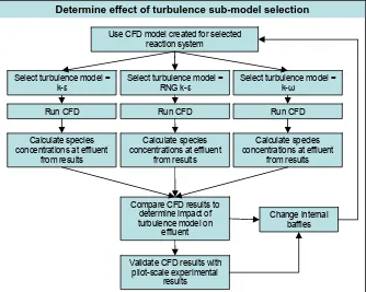
Figure 3.14: Determination of Turbulence Model Sensitivity... 81

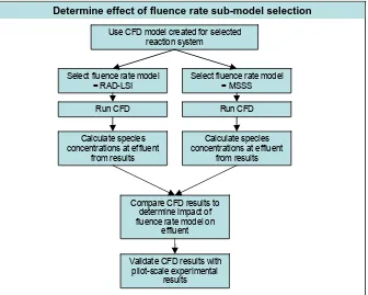
Figure 3.15: Determination of Fluence Rate Model Sensitivity... 82

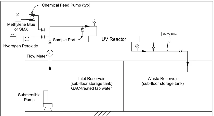
Figure 3.16: Low-Pressure UV Pilot System Schematic (NTS)... 84

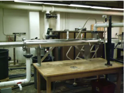
Figure 3.17: Overview of Pilot Reactor System ... 85

Figure 3.18: Baffle Plate from Reactor Interior... 85

Figure 3.19: Flow Meter for Pilot Reactor... 86

Figure 3.20: Pilot UV Intensity Sensor... 86

Figure 3.21: Pilot Chemical Feed System... 87

Figure 4.1: Competition Kinetic Data Plot for Kinetic Rate Constant Determination ... 99

Figure 4.2: Removal Rates as a Function of Hydrogen Peroxide Concentration (Collimated Beam at 50 mJ cm-2 and [MB]0 = 0.5 mg L-1) (a) Multiple Experiments in DI Water; (b) DI Water Results Compared to Pilot Influent Tank Water ... 103

Figure 4.3: Removal Rates as a Function of UV Dose (Collimated Beam) ... 104

Figure 4.4: Collimated Beam Baseline: Methylene Blue (MB) = 0.5 mg L-1, Hydrogen Peroxide = 0.0 mg L-1 (Trace lines added for clarity) ... 105

Figure 4.5: Initial Spectrophotometer Results for Methylene Blue in Pilot ... 106

Figure 4.6: Pilot Scale Results with No UV Irradiation ... 108

Figure 4.7: Pilot Results Showing No Direct Photolysis and Confirming Response to Hydrogen Peroxide Addition ... 109

Figure 4.9: Methylene Blue Pilot Reactor Results (One Baffle) ... 116

Figure 4.10: Sulfamethoxazole Pilot Test Results... 119

Figure 4.11: Velocity Distribution in Reactor with Five Baffles and Flow = 20 GPM... 122

Figure 4.12: Fluence Rate Distribution in Reactor (Output P = 29.6 W, UVT = 92.9 %) ... 122

Figure 4.13: Comparison of Pilot and CFD Results for Five-Baffle Trials... 128

Figure 4.14: Comparison of Pilot and CFD Results for One-Baffle Trials ... 129

Figure 4.15: Comparison of Pilot and CFD Results for SMX Trials... 134

Figure 4.16: Graphical Results of RAD-LSI Fluence Rate Sub-model in CFD in (a) Y-Z Plane and (b) X-Z Plane... 137

Figure 4.17: Graphical Results of MSSS Fluence Rate Sub-model in CFD in (a) Y-Z Plane and (b) X-Z Plane... 138

Figure 4.18: Impact of Second-Order Rate Constant on Methylene Blue Removal ... 141

Figure 4.19: Velocity Profiles for k-ε Turbulence Sub-Model at 20 GPM; (a) Y-Z Plane Contours and (b) Y-Z Vectors at Inlet ... 142

Figure 4.20: Velocity Profiles for RNG k-ε Turbulence Sub-Model at 20 GPM; (a) Y-Z Plane Contours and (b) Y-Z Vectors at Inlet ... 143

Figure 4.21: Velocity Profiles for k-ω Turbulence Sub-Model at 20 GPM; (a) Y-Z Plane Contours and (b) Y-Z Vectors at Inlet ... 144

Figure 4.22: Impact of DOC on Advanced Oxidation of Methylene Blue... 147

Figure 4.23: CFD and Pilot Cost Trends ... 151

Figure 4.24: AAC0 Fractions for Energy and Chemical Costs (CFD Results)... 153

Figure 4.25: Dose-Response Curves for 100 W Output Power ... 155

Figure 4.26: UV Dose Distribution for 20 GPM and 26.5 W Output Power ... 156

Figure 4.27: UV Dose Distribution for 20 GPM and 100 W Output Power ... 157

Figure 4.28: Dose Distributions on Common Axes... 158

1. INTRODUCTION

The use of ultraviolet-initiated (UV-initiated) advanced oxidation processes (AOP) is rapidly becoming an attractive alternative for the degradation of harmful organic contaminants that are not easily removed using conventional water treatment processes. UV-initiated AOPs include the combinations of UV/hydrogen peroxide (H2O2), UV/ozone, and

UV/heterogeneous catalyst (such as titanium dioxide). The focus of this research was the UV/H2O2 process with the goal that the methods and models developed herein can be

modified for other UV-initiated AOP processes. Design and optimization of UV/H2O2

systems include both system configuration (reactor design, pipe and fittings, lamp number, and lamp orientation) and chemical kinetics (reaction mechanisms and kinetic rate constants). While some numerical techniques have been developed for understanding UV/AOP performance, these techniques are limited in their applicability for analyzing full-scale UV/AOP systems while incorporating both reactor design and chemical kinetics. As a result, engineers and other water professionals need more appropriate numerical tools to use as part of the design process and in optimizing UV/AOP systems.

developed that is sensitive to these issues for proper simulation of UV-initiated AOP performance.

1.1 Originality and Relevance

Researchers have previously demonstrated the importance of combining UV reactor hydraulics with dynamic fluence rate models to predict the effectiveness of the disinfection process. The authors of a recent AwwaRF study that successfully applied UV-initiated advanced oxidation for the degradation of organic contaminants recognized the dependence on non-ideal reactor characteristics (hydrodynamics and fluence rate) for the overall AOP performance (Linden et al., 2004). Sharpless and Linden (2003) concluded that development of a predictive UV/AOP model that incorporates reactor hydraulics would allow design simulations that optimize lamp placement, minimize light screening, and improve prediction of contaminant removal in different UV reactors. However, no currently published research has applied CFD models to UV-initiated advanced oxidation reactors that experience non-ideal fluence rate and reactor hydraulic conditions. The objective of this research is to begin to develop the protocol for using CFD models to simulate UV-initiated AOPs.

as oxidation pathways for emerging contaminants are identified, a simulation model, such as the one described by this research, will become an important tool for the evaluation, design, and optimization of advanced oxidation systems. This research lays the groundwork for an improved design process and will provide a foundation for the future needs of the water treatment community.

Finally, utilities that integrate UV-initiated advanced oxidation into their treatment processes may also qualify for disinfection (log-kill) credit within the UV reactor. Since this will be uncharted territory for regulators, data from validated models will be critical in awarding disinfection credit within an AOP. Additional studies that combine the advanced oxidation models generated within the proposed research with UV disinfection models previously validated by others (e.g., Ducoste and Linden, 2005) will be the next logical step to achieve accurate simulation of performance of both advanced oxidation reactions and disinfection by UV reactors.

1.2 Hypotheses

The following four hypotheses were proposed to support the principal objective of this research:

here to distinguish the turbulence and fluence rate models (now called sub-models) from the overall CFD simulation (model).]

2. For the modeling of organic contaminant degradation, turbulence sub-model selection will impact the effluent concentrations of the contaminant and its oxidation byproducts predicted by CFD simulations of UV-initiated AOP reactors.

3. Incorporation of micromixing sub-models will improve the predictions of CFD models of fast reactions occurring in an AOP reactor.

4. A comprehensive CFD model for UV-initiated AOP reactors will allow designers to optimize energy and chemical usage to achieve a given degradation goal for organic contaminants.

2. LITERATURE REVIEW 2.1 Ultraviolet Photochemistry

Ultraviolet photochemistry can be defined as a chemical reaction, or a series of chemical reactions, that is initiated and/or driven by the absorption of ultraviolet radiation by one or more reactants. The ability of a reactant to absorb UV radiation is defined by its molar absorption coefficient (ελ, units of L mole-1 cm-1), a value unique to the reactant

molecule, or its absorbing functional group, that comprises a measure of an electronic transition probability (Ollis, 2003).

UV photochemistry is also dependent on the energy of the UV light incident on the reacting molecule. The magnitude of energy within a photon of UV light is described by Planck’s equation, which can be expressed as follows (Braun et al., 1991):

λ ν hc h

E= = (2-1)

where, E = energy, J • photon-1

h = Planck’s constant, 6.6256 x 10-34 J • s • photon-1 c = speed of light, 2.9979 x 108 m • s-1

λ = wavelength of radiation, m

Multiplying the energy per photon as calculated in Equation 2-1 by Avogadro’s number (6.023 x 1023) results in the energy per einstein, where an einstein is defined as one mole of photons. The effectiveness of a photochemical reaction may then be defined by a quantum yield Φ, which represents the moles of a given species photochemically transformed (reactant or product) per mole of photons (einstein) absorbed.

In this research, the chemical reactants were diluted in an aqueous medium. The Beer-Lambert law describes light transmission through an absorbing medium and is defined for a monochromatic light as (Braun et al., 1991),

lc -εlc 0

e 10 P

P

T= = − = κ _(2-2)

where, T = transmittance (typically expressed as a fraction)

P = transmitted power, e.g., W; or power per unit surface area, e.g., W • cm-2 P0 = incident power, e.g., W; or power per unit surface area, e.g., W • cm-2

ε = molar absorption coefficient, L • mol-1 • cm-1

l = thickness of solution traversed by light, cm (path length) c = molar concentration of absorbing species, mol • L-1

For polychromatic light, each of the terms in Equation 2-2, with the exception of path length and molar concentration, is expressed at a fixed wavelength. Absorbance may then be defined as,

variables) Napierian

for

κlc -lnT A (or

εlc logT

-A = = = = (2-3)

Absorbance follows the additive property, and if there are multiple absorbing species in the solution, then absorbance is defined as,

∑

i i i

l c

ε

A (2-4)

In Equation 2-2, the term for power (P) is used somewhat generically. To be more exact, the field of photochemistry has adopted specific definitions for terms associated with power from light. Bolton (2001) differentiates these terms as described below:

Radiant Power (P, W): The total radiant power emitted in all directions by a light source.

Radiant Intensity (I, W • sr-1_{): The total radiant power emitted by a source in a given direction}

about an infinitesimal solid angle dΩ.

Irradiance (E, W • m-2): The total radiant power incident from all upward directions on an infinitesimal element of surface of area dS containing the point under consideration, divided

Fluence Rate (E’, W • m-2_{): The total radiant power incident from all directions onto an}

infinitesimally small sphere of cross-sectional area dA, divided by dA.

Fluence (H’, J • m-2_{): The total radiant energy of all wavelengths passing from all directions}

through an infinitesimally small of cross-sectional area dA, divided by dA. Fluence is also

referred to as UV Dose.

For a constant fluence rate, the fluence (or UV dose) equals the fluence rate multiplied by the exposure time.

Although these terms are often used interchangeably, which as the definitions imply is incorrect, it is important that a reader understand what light concept is being discussed. For the remainder of this document, the terms as defined by Bolton (2001) will be used.

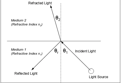
Since the UV light in a water treatment reactor passes through multiple media (i.e., air, quartz, and water), several of the laws of optics are applicable. Refraction describes the change in delivery angle (bending) of light as it passes through media with different refractive indices. The refraction is quantified using Snell’s Law, which relates incident angle, refractive angle, and refractive indices as follows:

2 2 1

1sinθ n sinθ

n = (2-5)

Light Source

θ

θ

θ

Medium 2

(Refractive Index n2)

Medium 1

(Refractive Index n1)

Incident Light

Reflected Light

Refracted Light

Figure 2.1: Relationship Among Incident, Refracted, and Reflected Light

As is shown in Figure 2.1, a portion of the incident light is reflected away from the interface between the two media. The reflectance is defined by the Fresnel Laws and can be quantified with Equation 2-6.

(

)

1

⊥

+

= r r

R _II (2-6)

where R = Reflectance,

II

r = Amplitude of radiant energy parallel to the plane of incidence, and

⊥

The two amplitudes shown in Equation 2-6 are defined in Equations 2-7 and 2-8. 1 2 2 1 2 1 1 2 cos cos cos cos θ θ θ θ n n n n r_II + − = (2-7) 2 2 1 1 2 2 1 1 cos cos cos cos θ θ θ θ n n n n r + − = ⊥ (2-8)

Both Snell’s Law and Fresnel’s Law will be used in the description of the fluence rate models in Section 2.6.

2.2 Advanced Oxidation

Advanced oxidation is the use of a powerful oxidizing agent (e.g., the hydroxyl radical •OH) to oxidize chemical compounds (Bolton, 2001). These compounds are primarily organic pollutants and can be oxidized in water, in air, or on the surface of solids. The term “advanced” describes the process of artificially creating the oxidant radicals to accelerate a reaction that could naturally occur in the environment if given time. In the UV/H2O2 AOP, the hydrogen peroxide molecule produces two hydroxyl radicals when

A significant amount of experimental research has been completed to evaluate the degradation of an organic species (parent compound) by UV-initiated advanced oxidation reactions (Sharpless and Linden, 2003; Bali et al., 2003; Devlin and Harris, 1984; Scheck and Frimmel, 1995). In other research studies, investigators have performed more detailed experiments to ascertain the reaction pathways involved in the degradation of the parent compound to its intermediate and final products (Stefan et al., 1996; Stefan et al., 2000; Alnaizy and Akgerman, 2000). The determination of these reaction pathways provides a more detailed picture of the photoreactive process and allows the development of numerical kinetic models that predict the rate of conversion of reactants to products. Detailed reaction pathways are very specific to the parent compound and chemical constituents in the water. However, once the reaction pathway is defined, researchers can combine the reaction kinetics of these UV-initiated AOPs with simulation models that describe the hydraulic and turbulent characteristics of a UV reactor system. Example advanced oxidation reaction mechanisms are described in Section 2.7.

UV-initiated advanced oxidation research has been performed using both low- and medium-pressure UV lamps. Sharpless and Linden (2003), in their study of direct photolysis and UV/H2O2 advanced oxidation for the degradation of NDMA in a synthetic water,

One of the recommendations by Sharpless and Linden (2003) was that a detailed hydraulic model coupled with an irradiance distribution profile be developed to examine the effect of optical path length and multiple-lamp reactors for UV/H2O2 systems. This research attempts

to complete this coupling of hydrodynamics and fluence rate distribution for advanced oxidation reactions in low-pressure UV reactors.

2.3 Computational Fluid Dynamics

Computational Fluid Dynamics (CFD) is a technique for numerically solving the equations of fluid dynamics over both space and time, including the conservation of mass, conservation of momentum, and conservation of energy. Combined with appropriate boundary and initial conditions, these governing equations can describe both the physical and chemical changes within a reactor. A CFD model for UV systems also includes the spatial variations of fluence rate within the UV reactor.

Limited studies have been performed with CFD to simulate UV/AOPs. Pareek et al. (2003) used CFD combined with a discrete-ordinate radiation transport equation for light intensity and modified k-ε turbulence equations to model a heterogeneous, multi-phase photocatalytic reactor system for the photodegradation of a spent Bayer liquor. However, the applied radiation model did not incorporate refraction and was performed in a simple bench scale reactor. Mohseni and Taghipour (2004) used CFD to evaluate the heterogeneous photocatalytic oxidation of gas-phase vinyl chloride (VC) by the UV initiation of a TiO2

-coated surface; however, this research did not incorporate a fluence rate model and only described the flux of VC toward the TiO2-coated surface. No research has been performed

As mentioned previously, the equations of fluid dynamics include the conservation of mass, conservation of momentum, and conservation of energy. For an incompressible fluid, the equation for the conservation mass, or the continuity equation, can be written as,

0 = ∂ ∂ + ∂ ∂ + ∂ ∂ z u y u x

u_x y _z

(2-9)

In equation 2-9, ux, uy, and uz are the velocity components in the x, y, and z directions, respectively. The conservation of momentum equations for turbulent flow are expressed for incompressible flow and no free surface (no gravity term) as the Reynolds-averaged Navier-Stokes equation (Clark, 1996):

( )

i _uu

x x x U x p x U U t

U _{′ ′}

∂ ∂ − ∂ ∂ ∂ + ∂ ∂ − = ∂ ∂ + ∂ ∂ _{ρ μ ρ}

ρ 2 (2-10)

where ρ is the fluid density, U_iis the average velocity in the i-th direction, t is time, pis the average pressure, μ is the absolute viscosity, and '

i

The last term on the right side of Equation 2-10, representing the Reynolds stresses, creates a closure problem for turbulence since it introduces additional unknowns that outnumber the equations available for solution. Thus, in order to numerically solve turbulence problems, new equations or models must be established such as the two-equation models described in Section 2.4.

The reactive turbulent convective-diffusion equations for species transport are shown in the equations below (Liu and Ducoste, 2006):

i j i T j j i j i _R x C D D x x C U t C + ⎟ ⎟ ⎠ ⎞ ⎜ ⎜ ⎝ ⎛ ∂ ∂ + ∂ ∂ = ∂ ∂ + ∂ ∂ ) ( (2-11)

where Ci is the average concentration of species i, U is the mean velocity, D is the molecular diffusivity coefficient, Ri is the reaction term for species i, and DT is the turbulent diffusivity that is defined as,

T T T

Sc

D = ν . (2-12)

In Equation 2-12, νT is the turbulent eddy viscosity and ScT is the turbulent Schmidt number, which, as seen upon rearrangement of Equation 2-12, may be defined as the ratio of the eddy

diffusivity of momentum (eddy viscosity) to the eddy mass diffusivity. The i T j C D x ⎛_∂ ⎞ ⎜ ⎟ ⎜_∂ ⎟ ⎝ ⎠ term

velocity. In this research, the reactions describing the advanced oxidation process wereused in the turbulent convective-diffusion equation to describe the reactive transport of each species throughout the flow domain.

2.4 Turbulence Models

Typically, full-scale UV photoreactors will operate in a turbulent flow regime, and thus, simulations of a UV process must incorporate the impact of turbulent mixing on any chemical reactions that occur within these UV photoreactors. Although the standard k-ε

models: 1) standard k-ε, 2) RNG k-ε, and 3) k-ω. The goal of using multiple sub-models is to determine the CFD model sensitivity to the turbulence sub-model selection. While other more complicated turbulence models exist, such as the Reynolds Stress Model or Large Eddy Simulation model, the three two-equation models selected for this research provide reasonable and stable results without being numerically intensive.

The standard k-ε model used in this study was proposed by Launder and Sharma (1974) (as cited in Wilcox 2004) to solve the turbulence stress closure problem. This model, as described by Wilcox (2004), is shown below (reference Table 2.1 for definition of variables):

ε ν Cμk2

T = (2-13)

⎥ ⎥ ⎦ ⎤ ⎢ ⎢ ⎣ ⎡ ∂ ∂ ⎟⎟ ⎠ ⎞ ⎜⎜ ⎝ ⎛ + ∂ ∂ + − ∂ ∂ = ∂ ∂ + ∂ ∂ j k T j j i ij j j x k x x U x k U t k σ ν ν ε

τ (2-14)

⎥ ⎥ ⎦ ⎤ ⎢ ⎢ ⎣ ⎡ ∂ ∂ ⎟⎟ ⎠ ⎞ ⎜⎜ ⎝ ⎛ + ∂ ∂ + − ∂ ∂ = ∂ ∂ + ∂ ∂ j T j j i ij j j x x k C x U k C x U t ε σ ν ν ε τ ε ε ε ε ε ε 2 2

1 (2-15)

k C_μ ε ω= ε μ 2 3 k C

l= (2-17)

The second closure model used in this study, the Renormalized Group (RNG) k-ε

model, was developed by Yakhot and Orszag (1986) using techniques from the renormalization group theory. In the RNG k-ε model, νT, k, and ε are still defined as in the

standard k-ε model. However, the RNG k-ε model uses modified coefficients and empirical constants to reduce the higher level of dissipation that is predicted using the standard k-ε

model. Thus, equations 2-13, 2-14, and 2-15 are still applicable. The closure coefficients are replaced by the following (Wilcox, 2004):

3 0 3 2 2 1 1 ~ βλ λ λ λ μ ε ε ₊ ⎟⎟ ⎠ ⎞ ⎜⎜ ⎝ ⎛ − + = C C

C (2-18)

ji ijS S k 2 ε

λ= (2-19)

Cε1=1.42, C~_ε2=1.68, Cμ=0.085, σk=0.72, σε=0.72, β=0.012, λ0=4.38 (2-20)

Wilcox in 1998, in which changes were made to the values of α, β0, and the dissipation terms

(β* and β) and the functions fβ and fβ* were added, the k-ω (98) model was found to predict

the experimental spreading rates reasonably well for all free shear flows, including far wake, mixing layer, and jet flows. The k-ω (98) model is described below (Wilcox, 2004):

ω

ν_T = k (2-21)

(

)

k _{τ β}* _{ω ν σ}*_{ν (2-22)}

(

)

ω 2 _(2-23)

α=13/25, β=β0fβ, β∗ =β₀∗f_β∗, σ=0.5, σ

*_{=0.5, β}

0=9/125, β₀∗ =0.09 (2-24)

ω ω β _χ χ 80 1 70 1 + + =

f , where

( )

= ij jkSki _(2-25)

⎪⎭ ⎪ ⎬ ⎫ ⎪⎩ ⎪ ⎨ ⎧ > + + ≤ = ∗ 0 400 1 680 1 0 1 2 2 k k k k f _χ χ χ χ

β , where

j j k x x k ∂ ∂ ∂ ∂ = ω ω

k ω β ε ₌ ∗ ω 2 1 k

l= (2-27)

⎟ ⎟ ⎠ ⎞ ⎜ ⎜ ⎝ ⎛ ∂ ∂ − ∂ ∂ = Ω i j j i ij _x U x U 2 1 (2-28) ⎟ ⎟ ⎠ ⎞ ⎜ ⎜ ⎝ ⎛ ∂ ∂ + ∂ ∂ = i j j i ij x U x U S 2 1 (2-29)

Variables that have not been previously defined but that are used in the three turbulence models are defined in Table 2.1.

Table 2.1: Variables in Turbulence Closure Sub-models

Symbol Definition

νT kinematic eddy viscosity k turbulent kinetic energy

ε turbulent energy dissipation

τij Reynolds stress tensor

ν kinematic molecular viscosity

ω specific dissipation rate (dissipation per unit turbulence kinetic energy)

l turbulence length scale Sij mean strain rate tensor

Ωij mean rotation tensor

two-solve the k-ε singularity problem at wall boundaries (where k approaches zero) and reduces the higher level of dissipation that is predicted using the Standard k-e model. However, the RNG k-ε is not as accurate in predicting free-shear (no wall) flows. The k-ω has been proven relatively accurate for boundary layer (i.e., wall bounded) flows and, with the 1998 revisions, also works well for free-shear flows.

2.5 Mixing Models

Contaminant oxidation, like all basic chemical reactions, requires spatial adjacency between (or among) the reacting molecules, which in this case, are initially the hydroxyl radical and the organic compound. In a typical system, the concentration of hydroxyl radicals will be much less than that of the target contaminant. Further, the reactions for radical formation and many of the oxidation reactions can be considered fast reactions. Thus, the physical process of mixing within the advanced oxidation reactor will be an important factor in determining the level of contaminant degradation. Researchers have shown that turbulent heterogeneity requires more attention than Magnussen and Hjertager’s minimum reaction kinetics approach when dealing with turbulent chemical reactions (Baldyga and Bourne, 1999; Spalding, 1998; Marchisio and Barresi, 2003). For this reason, the incorporation of mixing models in the CFD code should improve the accuracy in predicting effluent concentrations of the advanced oxidation products.

macromixing, mesomixing, and micromixing (Baldyga and Pohorecki, 1995; Baldyga and Bourne, 1992). Macromixing, or bulk blending, is the mixing process on the dimensional scale of the reactor as a whole and determines the environment for mesomixing and micromixing (Baldyga and Pohorecki, 1995). Mesomixing constitutes the localized reaction zone, which is a coarse scale relative to the micromixing, but is finer than the macroscale. Further, mesomixing represents the inertial-convective disintegration of large eddies (Baldyga and Pohorecki, 1995). Finally, micromixing is the scale of mixing that occurs within small eddies and signifies the viscous-convective deformation and engulfment process of fluid elements, which is the key physical process for mixing-sensitive chemical reactions (Rohani and Baldyga, 1987). Larger scale mixing such as macro- and mesoscale can be calculated using CFD codes directly. However, a specialized micromixing sub-model must be separately coded within CFD to simulate the mixing at this molecular scale, which is typically smaller than the CFD grid size.

Bourne, 1992; Rohani and Baldyga, 1987; Baldyga and Rohani, 1987). Although Baldyga and Rohani (1987) identify limitations of various micromixing models (e.g., the effects of turbulent circulation near inlet streams), it is clear that the inclusion of a micromixing model in a CFD simulation of UV-initiated AOPs must be investigated for accurate prediction of reaction results.

Several micromixing models have been developed, each intending to simulate the elementary process(es), i.e., eddy disintegration, engulfment, deformation, and/or molecular diffusion, which best describes mixing under the conditions presented. Baldyga and Bourne (1990) compare a simplified engulfment micromixing model (Baldyga and Bourne, 1989) with the interaction-by-exchange-with-the-mean (IEM) model, which differ by a static (IEM) versus growing (engulfment) localized reaction zone. Micromixing models also can be modified to capture the impact of the fragmentary and intermittent nature of turbulence on local chemical reactions (Baldyga and Pohorecki, 1995).

Equation 2-11, as presented previously, is considered the basis for the single fluid model (SFM) approach because the average concentration of each chemical species is defined by a scalar variable that is then convected and diffused by turbulent motion. In Equation 2-11, the chemical kinetic reaction rate for species i in reaction k is expressed as (Liu and Ducoste, 2006):

∏

reactant

j j

j i

ki

M X KM

where Mi is the molecular weight of product species i, ρ is the fluid density, Xj is the mass concentration of reactant species j, Mj is the molecular weight of reactant species j, and K is the reaction kinetic rate constant.

For turbulent chemical reaction conditions, a turbulent mixing rate must also be included in the reaction process (Baldyga and Bourne, 1992; Bakker et al., 2001). Several models have been proposed to describe the turbulent effects on heat/mass transfer and chemical reaction, including the eddy-break-up model, the eddy dissipation concept, and two-fluid (or multi-fluid) models. For the single fluid model approach in this study, the turbulent mixing rate was based on the eddy-dissipation concept (Forney and Nafia, 1998; Hjertager et al., 2002). The method for calculating the overall reaction rate in the SFM approach was based on Magnussen and Hjertager’s model (Bakker et al., 2001) where the overall reaction rate term Ri is calculated as the minimum between the chemical kinetic reaction rate, Rki, and the turbulent mixing rate, Rmi, as follows (Liu and Ducoste, 2006):

(

)

i R R

R =−ν min , (2-31)

where νi is defined as the stoichiometry of species i and is positive for reactants and negative

for products. The turbulent mixing rate is described by the following:

⎟ ⎟ ⎞ ⎜

⎜ ⎛

⎟ ⎟ ⎞ ⎜

⎜ ⎛ • ⎟ ⎠ ⎞ ⎜

⎝ ⎛

= _{i mn} min j

mi

M X k

A M R

ν ρ ε

where νj is defined as the stoichiometry of species j, Amn is an empirical constant that varies

between 1 and 5 with a nominal value of 2.5 (Hjertager et al., 2002), ε is the dissipation of turbulent kinetic energy, and k is the turbulent kinetic energy. The interpretation of Magnussen and Hjertager’s model and Equation 2-32 is that (i) in regions of low mixing intensity and for fast reactions, the overall reaction rate is limited by the mixing rate, and (ii) in regions of high mixing intensity, the chemical kinetic rate is the limiting factor.

2.6 Fluence Rate Models

In Section 2.1, the UV fluence rate (incident radiant power) was shown to vary with distance from the lamp and as a function of the absorptive characteristics of the media through which the light passes. In advanced oxidation reactions, both the organic contaminant and H2O2 absorb UV light, reducing the transmitted fluence rate, and

Stamnes et al., 1988; Liou and Wu, 1996). Liu et al. (2004) directly evaluated the performance of these models with experimental measurements of the fluence rate at different points within a UV reactor, the results being a compilation of the strengths and weaknesses of the each model’s ability to predict the fluence rate. Ducoste and coworkers further showed that the microbial log inactivation and the shape of the fluence distribution were sensitive to the fluence rate model selection (Ducoste et al., 2005; Liu et al., 2006). Their results suggest the need to evaluate the influence of the fluence rate model selection on any photoreactive process such as UV-initiated advanced oxidation processes.

The RAD-LSI and MSSS models were chosen to simulate the fluence rate in this study and to determine the influence of this selection on the predicted effluent concentrations from a UV/AOP process. These two models were selected based on their performance in predicting the UV light distribution in Liu et al. (2004) and the ease of incorporation into a CFD model simulation. The RAD-LSI is a modified version of the line source integration model (Blatchley, 1997) that was enhanced to account for the physics of reflection, refraction, and absorption and provides better prediction of the fluence rate near the lamp surface using the radial model component (Liu et al., 2004). The RAD-LSI model is represented by Equations 2-33 and 2-34:

(

)

2 arctan 2 arctan 4 , 2 min ) , ( ' × ⎪⎭ ⎪ ⎬ ⎫ ⎪⎩ ⎪ ⎨ ⎧ ⎥ ⎥ ⎦ ⎤ ⎢ ⎢ ⎣ ⎡ ⎟ ⎟ ⎠ ⎞ ⎜ ⎜ ⎝ ⎛ ₋ + ⎟ ⎟ ⎠ ⎞ ⎜ ⎜ ⎝ ⎛ ₊ = r h L r h L Lr P Lr P h r E π

(

)

(

)(

) (

)

(

)

∑

∑

k k k

d q d w k k k k k h r n P T T d d d n P R R k k 1

1 2 2

01 . 0 01 . 0 2 , 3 , 2 , 1 , 2 , 1 4 4 1 1 factor atten , 2 , 3 π π (2-34)

The variables used in Equations 2-33 and 2-34 are defined as follows:

• E’(r,h) is the fluence rate at a point in the reactor with normal (perpendicular) distance r to the lamp axis and longitudinal distance h to the lamp center.

• Pλ is the radiant power at wavelength λ uniformly emitted in all directions by the

point source.

• L is the total length of the lamp.

• R1 is the reflectance factor for the air/quartz interface (see Equation 2-6). • R2 is the reflectance factor for the quartz/water interface (see Equation 2-6). • Tw is the 10-mm path length transmittance of the water.

• Tq is the 10-mm path length transmittance of the quartz. • d1 is the path length in the air (see Figure 2.2).

• d2 is the path length in the quartz (see Figure 2.2). • d3 is the path length in the water (see Figure 2.2).

θ₃

θ₁

θ₂d2,k

θ₂d2,k

d_3,k

d_1,k

Lamp Centerline Lamp Edge

Air (na)

Quartz Sleeve (nq,Tq)

Reactor Wall

Water (n_w,T_w)

Lamp “Point” k

h_k

r_k

R

eactor R

adi

us

r₁ r₃

r₂

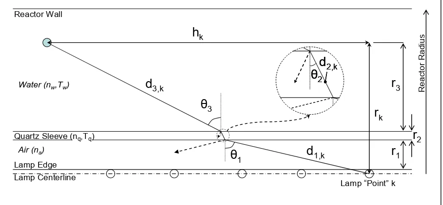
Figure 2.2: Angle Geometry of Attenuation Factor in RAD-LSI Model

In Figure 2.2, the normal distance between the lamp centerline to the inner edge of the quartz sleeve is defined as r1, the thickness of the quartz sleeve is r2, and the normal

distance from the outer edge of the quartz sleeve to the point of interest is r3. Using these

terms and the incident angles shown in Figure 2.2, the distance hk can be defined as shown in

Equation 2-35.

3 , 3 2 , 2 1 ,

1ktanθ ktanθ ktanθ

k r r r

h = + + (2-35)

⎟ ⎟ ⎠ ⎞ ⎜ ⎜ ⎝ ⎛ = − 1 1

2 sin sinθ

θ q a n n (2-36) ⎟⎟ ⎠ ⎞ ⎜⎜ ⎝ ⎛ = − 1 1

3 sin sinθ

θ w a n n (2-37)

In equations 2-36 and 2-37, na, nq, and nw are the refractive indices for air, quartz, and

water, respectively. The path lengths d1, d2, and d3 in the RAD-LSI equations are determined

using trigonometry and previously defined variables as shown in equations 38, 39, and 2-40.

1 1

1 _cosθ

r

d = (2-38)

2 2

2 _cosθ

r

d = (2-39)

3 3

3 _cosθ

r

d = (2-40)

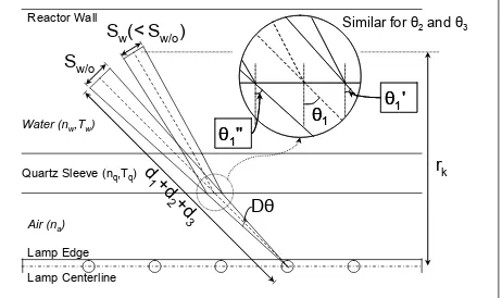
corrected by modeling the lamp as a series of differential cylindrical segments, where light is emitted normal to the cylinder surface and decreases with the cosine of the angle between the unit normal and the direction vectors (Liu et al., 2004). This fluence rate modeling approach is called the multiple segment source summation (MSSS). The MSSS fluence rate at a specific point in space caused by the UV light emitted from a segment source is described as (Liu et al., 2004):

(

)

) ( 4 / ) 1 )( 1

( /0.01 /0.01 ₁

2 3 2 1 2

1 _π 3 2 _π⎟ θ

⎠ ⎞ ⎜ ⎝ ⎛ + + − −

= T T focus

d d d n P R R I d q d w

A (2-41)

The focus factor in Equation 2.41 is defined as the ratio of surface areas for the conical frustums with axes on the lamp centerline and slant heights of Sw and Sw/o shown in Figure 2.3. This ratio is defined numerically in Equation 2-42.

(

)

(

)

1 2 3 2 1 cos ' '' cos ) ( θ θ θ h h r d d d focus − Δ + +

Lamp Centerline Lamp Edge

Air (na)

Quartz Sleeve (n_q,T_q)

Water (nw,Tw)

Reactor Wall

r

d

1

+d

+d

3

D

θ

θ

θ

''

θ

'

θ

θ

''

θ

'

Similar for θ₂and θ₃

S

S

(< S

)

Figure 2.3: Geometry of Focus Factor in MSSS Model

2.7 Chemical Contaminants

2.7.1 Dye Decolorization

Table 2.2: Properties of Several Organic Dyes Dye Name/ Formula/ Description Molecular Weight CAS Registry Number Wavelength of Maximum Absorbance Second-Order Rate

Constant Ref

CI Acid Orange 7 (AO7) / C16H11N2NaO4S /

Monoazo anionic dye-acid class

350.32 633-96-5 485 nm NA (1)

Methylene Blue / C16H18ClN3S /

Azindyes 319.85 61-73-4 662 nm / 470 nm k = 1.2 × 10

10

k = 2.1 × 1010

(L mol-1 _s-1₎

(2, 8)

CI Reactive Red 141 /

Reactive azo dye 1781 NA 544 nm NA (3)

CI Reactive Black 5 /

Reactive diazo dye NA NA 583 nm NA (4)

Malachite Green (MG) / C23H26N2 /

Triarylmethane dye (cationic)

330.47 129-73-7 617 nm NA (5)

Acid Orange 52

(AO52; Methyl Orange) / C14H14N3NaO3S /

Hydrosoluble aminoazobenzenes

327.33 547-58-0 463 nm NA (6)

Xylenol Orange / C31H28N2Na4O13S

(sodium salt) / Sulfonephyhalein dye

760.59 3618-43-7 580 nm k/kreference = 25

k = 2.4 × 1010

(L mol-1 _s-1_),

kreference = 9.7 × 108

(L mol-1 _s-1_),

pH = 11

(7)

NA = Not Available

References: (1) Behnajady and Modirshahla (2006); Behnajady et al. (2004) (2) Banat et al. (2005)

(3) Gultekin and Ince (2004)

(4) El-Dein et al. (2001)

(5) Modirshahla and Behnajady (2006)

(6) Galindo et al. (2000)

(7) Gupta and Hart (1971)

(8) Radiation Chemistry Data Center (RCDC), Notre Dame Radiation Laboratory, Online database

2 2 2

H O +hν → iOH (2-43)

[

]

2 2 2 2

'

2 2 2

UV H O CFD H O

r = Φ E ε H O (2-44)

In Equation 2-44,

2 2

H O

Φ is the quantum yield for the photolysis of hydrogen peroxide (moles H2O2 per mole photons, or moles H2O2 per einstein) and ε_{H O2 2} is the molar absorptivity of

hydrogen peroxide (L mol-1 _cm-1_{). The square brackets [] represent the molar concentration}

of the species enclosed in the brackets. The term '

CFD

E is the irradiance (UV@254 nm) at each individual grid cell centerpoint in the CFD domain. Since the light distribution models result in an irradiance term in units of W m-2_{, a unit conversion is necessary for the r}

UV term.

Noting that the variable C3 is used within the CFD code to represent the irradiance at each

grid location, the term '

CFD

E can be defined as shown in Equation 2-45.

( )

( )

(

)

( )

2 3 '

3 254

100 1000

CFD

W cm

C _m

m E

J L

U _Einstein

m ×

=

× (2-45)

Using this definition, rUV has units of moles L-1 s-1.

(

)

2 2 2 2 2

H O _+iOH _→H O HO_{+ i →}H+_+iO− _(2-46)

7 1 1

1 2.7 10

k = × M s− − (Buxton et al., 1988) (2-47)

[

]

_[

_][

_]

1 2 2

d H O

k H O OH

dt = − i (2-48)

[

]

_[

_][

_]

1 2 2

d OH

k H O OH

dt = −

i

i (2-49)

[

][

]

2

1 2 2

d O

k H O OH

dt

−

⎡ ⎤

⎣i _{⎦ = i (2-50)}

Hydrogen peroxide reacts with the superoxide radical according to Equations (2-51) through (2-55).

2 2 2 2

H O +iO− →iOH O+ +OH− (2-51)

1 1

2 0.13

k = M s− − (Weinstein et al., 1979) (2-52)

[

]

_[

_]

2 2 2 2

d H O

k H O O

dt

−

⎡ ⎤

[

]

2

2 2 2 2

d O

k H O O

dt

−

−

⎡ ⎤

⎣ ⎦ _{= − ⎡ ⎤}

⎣ ⎦

i

i (2-54)

[

]

_[

_]

2 2 2 2

d OH

k H O O

dt

−

⎡ ⎤

= _{⎣ ⎦}

i

i (2-55)

The hydroxyl radical will recombine with itself to form hydrogen peroxide as shown in Equations 2-56 through 2-59.

2 2

OH+ OH →H O

i i (2-56)

9 1 1

3 5.5 10

k = × M s− − (Buxton et al., 1988) (2-57)

[

]

_[

_][

_]

3

d OH

k OH OH

dt = −

i

i i (2-58)

[

]

_[

_][

_]

3

d H O

k OH OH

dt = i i (2-59)

2 2

OH₊ O−_→O ₊OH−

i i (2-60)

9 1 1

4 7.0 10

k = × M s− − (Beck, 1969 as cited in Crittenden, et. al, 1999) (2-61)

[

]

_[

_]

4 2

d OH

k OH O

dt

−

⎡ ⎤

= − _{⎣ ⎦}

i

i i (2-62)

[

]

2

4 2

d O

k OH O

dt

−

−

⎡ ⎤

⎣ ⎦ _{= − ⎡ ⎤}

⎣ ⎦

i

i i (2-63)

Methylene blue (MB) degrades through reaction with the hydroxyl radical to form products not currently under investigation by this research, and thus, will be labeled as unknown in Equations 2-64 through 2-67. For the reaction rate constant defined in Equation 2-65, the reader may reference the competition kinetics process described in Section 3.4.1.

OH MB+ →Unknowns

i (2-64)

9 1 1

, 6.9 10

MB OH

k i = × M s− − (2-65)

[

]

_[

_{][ ]}

,

MB OH

d OH

k OH MB

dt = − i

i

[ ]

_[

_{][ ]}

,

MB OH

d MB

k OH MB

dt = − i i (2-67)

Several hydroxyl radical scavengers can also be expected in the background water matrix. These scavengers will consume radicals according to Equations 2-68 through 2-83.

Dissolved Organic Carbon (DOC):

DOC+iOH →Unknowns (2-68)

1

4 1

, 2.5 10

DOC OH

mg

k s

L

− −

⎛ ⎞

= × _{⎜ ⎟}

⎝ ⎠

i (Larson and Zepp, 1988) (2-69)

[

]

_[

_]

₍

₎

,

DOC OH

d OH

k OH DOC

dt = − i

i

i (2-70)

Alkalinity (which at neutral pH is dominated by the bicarbonate ion):

3 3 2

HCO−+_iOH →COi−+H O _{(Buxton et al., 1988) (2-71)}

3

6 1 1

, 8.5 10

HCO OH

[

]

_[

_]

3, 3

HCO OH

d OH

k HCO OH

dt −

−

⎡ ⎤

= − _{i ⎣ ⎦}

i

i (2-73)

Monochloramine:

2 2

NH Cl OH+i →iNHCl H O+ (Johnson et al., 2002) (2-74)

Or alternatively,

2 2

NH Cl OH+i →iNH +HOCl (Johnson et al., 2002) (2-75)

2

9 1 1

, (2.8 0.2) 10

NH Cl OH

k _i = ± × M s− − (Johnson et al., 2002) (2-76)

[

]

_[

_][

_]

2 , 2

NH Cl OH

d OH

k NH Cl OH

dt = − i

i

i (2-77)

Free chlorine:

2

HOCl+iOH →H O OCl+i (Watts et al., 2007) (2-78)

4 1 1

, 8.5 10

HOCl OH

k i = × M s− − (Watts et al., 2007) (2-79)

[

]

_[

_][

_]

,

HOCl OH

d OH

k HOCl OH

dt = − i

i

i (2-80)

9 1 1 , 8.8 10

OCl OH

k − M s

− −

= ×

i (2-82)

(Buxton and Subhani, 1972 as cited in Feng et al., 2007)

[

]

_[

_]

,

OCl OH

d OH

k OCl OH

dt −

−

⎡ ⎤

= − _{i ⎣ ⎦}

i

i (2-83)

To improve convergence within the CFD code, two modifications to the reaction equations have been made (and are included in this section for completeness). The first is that the four species being tracked were normalized to initial conditions. The second is that, since the lifetimes of the two radical species are very short, pseudo-steady-state conditions for the two radicals were assumed. For the normalization of the species concentrations, the following variables have been defined.

[

]

[

]

[

]

[

]

5 2 2 5 2 2 0

2 2 0 H O

C H O C H O

H O

= ⇒ = (2-84)

In Equation 2-84 and those following, the subscript “0” indicates the initial concentration of the species entering the UV reactor.

[ ]

[ ]

[ ]

[ ]

6 6 0

0 MB

C MB C MB

MB

[

]

[

]

[

]

[

]

7 7 2 2 0

2 2 0 OH

C OH C H O

H O

= i ⇒ i = (2-86)

[

]

[

]

8 2 8 2 2 0

2 2 0 O

C O C H O

H O −

−

⎡ ⎤

⎣ ⎦ _{⎡ ⎤}

= i ⇒ _⎣i _⎦= (2-87)

An example of the substitution of these variables into the kinetic rate equations is shown in Equations 2-88 and 2-89 for previously presented Equation 2-48.

[

]

_[

_][

_]

1 2 2

d H O

k H O OH

dt = − i (2-48)

[

]

[

] [

]

2 2 ₀ 1 5 2 2 ₀ 7 2 2 ₀

dC

H O k C H O C H O

dt = − (2-88)

[

]

5

1 5 2 2 0 7

dC

k C H O C

dt = − (2-89)

[

]

_[

_]

_[

_][

_]

[

]

[

][

]

[

]

[

][ ]

[

]

(

)

[

]

[

][

]

[

]

[

][

]

2 2 2 2

2 3

'

2 2 1 2 2

2 2 2 2 3 4 2

, ,

3 , 2

,

, ,

2 _{H O H O CFD}

MB OH DOC OH

NH Cl OH HCO OH

HOCl OH OCl OH

d OH

H O E k H O OH

dt

k H O O k OH OH k OH O

k OH MB k OH DOC

k OH HCO k OH NH Cl

k OH OCl k OH HOCl

ε − − − − − − = Φ − ⎡ ⎤ ⎡ ⎤ + _{⎣ ⎦}− − _{⎣ ⎦} − − ⎡ ⎤ − _{⎣ ⎦}− ⎡ ⎤ − _{⎣ ⎦}− i i i i i i i i

i i i i i

i i

i i

i i

(2-90)

Setting the change in radical concentration equal to zero, Equation 2-90 can be rearranged and written for the pseudo-steady-state hydroxyl radical concentration

[

]

[

] [

]

{

[

]

[ ]

(

)

[

]

[

]

}

[

]

[

]

2 2 2 2

2

3 1 2 2 4 2

, , 3

2

'

2 2 2 2 2 2

0

2

SS SS

MB OH DOC OH HCO

NH Cl OCl HOCl

H O H O CFD

k OH OH k H O k O

k MB k DOC k HCO

k NH Cl k OCl k HOCl

k H O O ε H O E

− − − − − − ⎡ ⎤ = − + − _{− ⎣ ⎦} ⎡ ⎤ − − − _{⎣ ⎦} ⎡ ⎤ − − _{⎣ ⎦}− ⎡ ⎤ + _{⎣ ⎦}+ Φ i i

i i i

i

(2-91)

Since this is a quadratic equation, it can be solved using the following equations:

3

A= −k (2-92)

[

]

[ ]

(

)

[

]

[

]

2 3

1 2 2 4 2 , ,

3 2

MB OH DOC OH

NH Cl HOCl

HCO OCl

k H O k O k MB k DOC

B

k − HCO k NH Cl k − OCl k HOCl

[

]

[

]

'

2 2 2 2 2 H O H O 2 2 CFD

C k H O= ⎡_⎣iO−⎤_⎦+ Φ ε H O E (2-94)

And

[

]

B B AC

OH

A

− ± −

=

i (2-95)

As an example of how Equations 2-92 through 2-95 are written into numerical code, Equation 2-96 displays the steady-state hydroxyl radical concentration in a linear format.

[•OH]SS = (-(((-k1*[H2O2])-(k4*[•O2-])-(kMB*[MB])-(kDOC*(DOC))-(kHCO3-*[HCO3-

])-(kNH2Cl*[NH2Cl])-(kOCl-*[OCl-])-(kHOCl*[HOCl])))-(((((-k1*[H2O2])-(k4*[•O2-

])-(kMB*[MB])-(kDOC*(DOC))-(kHCO3-*[HCO3-])-(kNH2Cl*[NH2Cl])-(kOCl-*[OCl-

])-(kHOCl*[HOCl])))^2-(4((-k3))(((k2*[H2O2]*[•O2-])+(2*ΦH2O2*

εH2O2*[H2O2]*ECFD)))))^0.5))/(2((-k3))) (2-96)

[

]

[

]

[

] [

]

[

] [

]

[

] [

]

[

] [

]

[

] [ ]

[

]

(

)

[

]

[

] [

]

2 2 2 2

3

2

' 7

2 2 0 5 2 2 0 1 5 2 2 0 7 2 2 0

2 5 2 2 0 8 2 2 0 3 7 2 2 0 7 2 2 0

4 7 2 2 ₀ 8 2 2 ₀ , 7 2 2 ₀ 6 ₀

, 7 2 2 _{0 ,} 7 2 2 ₀ 3

, 7 2 2 0 2 ,

2 _{H O H O CFD}

MB OH

DOC OH _{HCO OH}

NH Cl OH OCl O

dC

H O C H O E k C H O C H O

dt

k C H O C H O k C H O C H O

k C H O C H O k C H O C MB

k C H O DOC k C H O HCO

k C H O NH Cl k

ε − − − = Φ − + − − − ⎡ ⎤ − − _{⎣ ⎦} − − i i _i

i i

[

]

[

] [

]

7 2 2 0

, 7 2 2 0

H

HOCl OH

C H O OCl

k C H O HOCl

−

⎡ ⎤

⎣ ⎦

− _i

(2-97)

Dividing through by the initial concentration of hydrogen peroxide

[

]

[

]

[

]

[

]

[

]

[ ]

(

)

[

]

[

]

2 2 2 2

3

2

' 7

5 1 5 7 2 2 0 2 5 8 2 2 0

3 7 7 2 2 0 4 7 8 2 2 0 , 7 6 0

, 7 , 7 3

, 7 2 _, 7 , 7

2 _{H O H O CFD}

MB OH

DOC OH HCO OH

NH Cl OH _{OCl OH} HOCl OH

dC

C E k C C H O k C C H O

dt

k C C H O k C C H O k C C MB

k C DOC k C HCO

k C NH Cl k C OCl k C HOCl

ε − − − − = Φ − + − − − ⎡ ⎤ − − _{⎣ ⎦} ⎡ ⎤ − − _{⎣ ⎦}− i i i

i _i i

(2-98)

For the pseudo-steady-state assumption, the time rate change of C7 is set equal to

zero, and the equation solved for C7, which can then be identified as C7,SS as shown in