Scholarship at UWindsor
Scholarship at UWindsor
Electronic Theses and Dissertations Theses, Dissertations, and Major Papers
2012
Identifying MicroRNA Precursors Using Linear Dimensionality
Identifying MicroRNA Precursors Using Linear Dimensionality
Reduction With Explicit Feature Mapping
Reduction With Explicit Feature Mapping
Navid Shakibapour Tabrizi
University of Windsor
Follow this and additional works at: https://scholar.uwindsor.ca/etd
Recommended Citation Recommended Citation
Shakibapour Tabrizi, Navid, "Identifying MicroRNA Precursors Using Linear Dimensionality Reduction With Explicit Feature Mapping" (2012). Electronic Theses and Dissertations. 5410.
https://scholar.uwindsor.ca/etd/5410
This online database contains the full-text of PhD dissertations and Masters’ theses of University of Windsor students from 1954 forward. These documents are made available for personal study and research purposes only, in accordance with the Canadian Copyright Act and the Creative Commons license—CC BY-NC-ND (Attribution, Non-Commercial, No Derivative Works). Under this license, works must always be attributed to the copyright holder (original author), cannot be used for any commercial purposes, and may not be altered. Any other use would require the permission of the copyright holder. Students may inquire about withdrawing their dissertation and/or thesis from this database. For additional inquiries, please contact the repository administrator via email
MAPPING
by
Navid Shakibapour Tabrizi
A Thesis
Submitted to the Faculty of Graduate Studies through Computer Science
in Partial Fulfillment of the Requirements for the Degree of Master of Science at the
University of Windsor
Windsor, Ontario, Canada 2012
c
MAPPING
by
Navid Shakibapour Tabrizi
APPROVED BY:
Dr. S´ev´erien Nkurunziza, External Reader Mathematics and Statistics
Dr. Alioune Ngom, Internal Reader Computer Science
Dr. Luis Rueda, Advisor Computer Science
Dr. Robin Gras, Chair of Defense Computer Science
I hereby certify that I am the sole author of this thesis and that no part of this thesis has
been published or submitted for publication.
I certify that, to the best of my knowledge, my thesis does not infringe upon anyone’s
copyright nor violate any proprietary rights and that any ideas, techniques, quotations, or
any other material from the work of other people included in my thesis, published or
oth-erwise, are fully acknowledged in accordance with the standard referencing practices.
Fur-thermore, to the extent that I have included copyrighted material that surpasses the bounds
of fair dealing within the meaning of the Canada Copyright Act, I certify that I have
ob-tained a written permission from the copyright owner(s) to include such material(s) in my
thesis and have included copies of such copyright clearances to my appendix.
I declare that this is a true copy of my thesis, including any final revisions, as approved
by my thesis committee and the Graduate Studies office, and that this thesis has not been
submitted for a higher degree to any other University or Institution.
MicroRNAs are a class of small RNAs of about 20 nucleotides long, which regulate cellular
processes in animals and plants. Identifying microRNAs is one of the important tasks in
microRNA and transcriptional studies. The main signal that is used for identifying these
tiny molecules is the hairpin secondary structure of microRNA precursors.
In this research, I propose to use a linear dimensionality reduction(LDR)-based
clas-sifier to identify precursor microRNAs from both pseudo hairpins and other non-coding
RNAs. LDR has been shown to be widely used in machine learning and pattern
recogni-tion problems. Due to the complexity of the data and nature of the problem, linear-based
classifiers might not have an acceptable performance. Therefore, I propose to use explicit
mapping to project data onto a higher dimensional space in order to increase class
separa-bility. Feature selection methods are used in order to reduce the complexity of the classifier
and find relevant biological descriptors.
To my parents
and
to Vida
I am pleased to express my deepest sense of gratitude to Dr. Luis Rueda. His informative
guidance, continues support and worthwhile feedback helped me throughout the course of
this thesis. It was an honour to be supervised by him and I will always be grateful to him.
I would like to thank Dr. Alioune Ngom and Dr. S´ev´erien Nkurunziza for spending their
invaluable time. Their indispensable inputs and discussions greatly improved the quality of
this thesis.
I owe my parents a deep debt of gratitude. Without their unconditional love and support,
the very possibility of my ever succeeding in life would be doubtful.
Special thanks to my sister, Mahtab, for her consistent support.
I would also like to thank my friends Iman Rezaian, Gokul Vasudev, Manish Kumer
Pandit and our Pattern Recognition and Bioinformatics lab members for their moral support.
At the end, I would like to conclude by extending my sincere appreciation and express
my undying love to my dearest Vida. Thanks for making my life so beautiful.
Author’s Declaration of Originality iii
Abstract iv
Dedication v
Acknowledgements vi
List of Figures xi
List of Tables xii
List of Algorithms xiv
I
Background
1
1 Introduction 2
1.1 MicroRNA . . . 2
1.2 Classification . . . 3
1.3 Motivation and Objectives . . . 3
1.4 Problem . . . 6
1.5 Contributions . . . 6
1.6 Thesis Organization . . . 7
2 MicroRNAs 8 2.1 Gene Expression . . . 8
2.2 MicroRNA . . . 9
2.3 Biogenesis of MicroRNA . . . 9
2.4 MicroRNA Identification . . . 12
2.5 Related Works . . . 13
2.5.1 Focusing on Genome Regions Around Known MicroRNAs . . . 14
2.5.2 Local Contiguous Structure-sequence Information of Stem-loops . . 15
2.5.3 One-class Compared Two-class Classifiers . . . 16
2.5.4 Global and Intrinsic Folding Features . . . 17
2.5.5 Enhancing Global and Intrinsic Folding Features . . . 19
2.5.6 Co-learning of Sequence and Structure . . . 20
2.5.7 The Ranking Algorithm Based on Random Walks . . . 21
2.5.8 The Na¨ıve Bayes Algorithm . . . 22
2.5.9 The Random Forest Algorithm For Classification . . . 24
2.5.10 Structural Motifs . . . 25
2.5.11 The Kernel Density Estimation Algorithm . . . 26
2.5.12 Feature Selection via aGenetic Algorithm . . . 27
2.5.13 Sample Selection for Classification . . . 28
3 Dimensionality Reduction and Explicit Mapping 30 3.1 Dimensionality Reduction . . . 31
3.2 Feature Selection . . . 36
3.3 Classification . . . 38
3.3.1 Linear Classifier -ΣΣΣi=σ2I . . . 40
3.3.2 Quadratic Classifier -ΣΣΣi=arbitrary . . . 41
3.4 Non-linear Mapping of LDA . . . 42
3.4.1 Mapping with Linear Functions . . . 43
3.4.2 Mapping with the Gaussian Radial Basis Function . . . 44
3.5 K-fold Cross-validation . . . 46
3.6 Class Imbalance Problem and Performance Evaluation Challenge . . . 47
II
Methods
50
4 Proposed Methodology 51 4.1 Dataset . . . 514.1.1 Positive dataset . . . 51
4.1.2 Negative Dataset . . . 52
4.2 The Features . . . 52
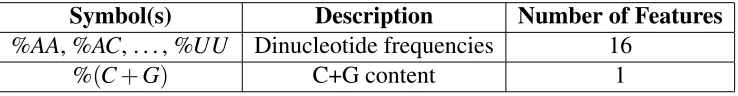
4.2.1 Primary Structure . . . 53
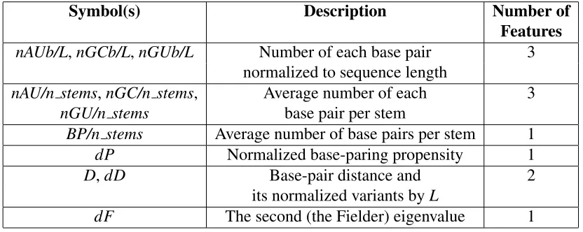
4.2.2 Secondary Structure . . . 54
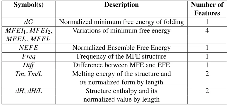
4.2.3 Energy Related . . . 56
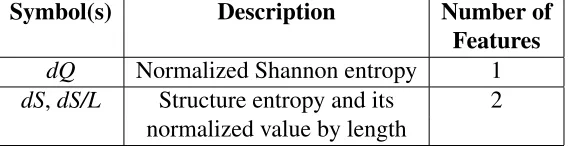
4.2.4 Information Theoretic . . . 57
4.2.5 Normalized Values . . . 58
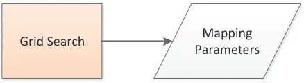
4.3 Model Flowchart . . . 58
4.3.1 Feature Selection . . . 58
4.3.3 Mapping Parameters . . . 60
4.3.4 LDA classifiers andK-fold Cross-validation . . . 61
4.3.5 Intermediate Results . . . 61
4.4 Optimizing Mapping Parameters . . . 63
III
Results and Discussion
64
5 Result and Discussion 65 5.1 Experimental Results . . . 655.2 Discussion and Comparison . . . 75
IV
Conclusions and Perspectives
78
6 Conclusions and Perspectives 79 6.1 Contributions . . . 806.2 Future Works . . . 80
V
Appendices
82
A Feature Indices 83
B How to Set Up the Classifier 84
Bibliography 86
1.1 MiRBase database growth between December 2002 and August 2012. . . . 5
2.1 The central dogma of molecular biology. . . 8
2.2 Secondary structure oflin-4. . . 10
2.3 The biogenesis of microRNAs. Figure is taken from [12] by authors’
per-mission. . . 11
4.1 Overall flowchart of the proposed system. . . 59
4.2 Optimizing Mapping Parameters. . . 63
5.1 Performance of the classifiers with different RBF parameters with features
21 and 25. . . 69
5.2 Performance of the classifiers with different RBF parameters with features
25 and 26. . . 70
5.3 Performance of the classifier at different stages of Alg. 1 with different
number of features. . . 74
4.1 Primary structure features. . . 53
4.2 Secondary structure features. . . 54
4.3 Energy related features. . . 56
4.4 Information theoretic features. . . 58
4.5 Normalized features. . . 58
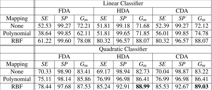
5.1 Classification performance for different combinations of LDA methods cou-pled with linear and quadratic classifiers. Each row represents the best per-formance in term ofGm of the classifier when using none, polynomial and RBF mapping function. . . 66
5.2 Performance of the classifier at different stages of Algorithm 1 with differ-ent numbers of features. . . 67
5.3 Classifier performance for the top 10 subset of feature. . . 71
5.4 Performance of the classifier after optimization of mapping parameters for three and seven features. . . 75
5.5 Comparison between miLDR-EM with just three features and previously proposed methods. . . 76
5.6 Comparison the performance of miLDR-EM and different feature selection algorithms used in microPred. . . 76
1 Feature selection algorithm. . . 38
2 Explicit mapping with Gaussian RBF . . . 45
Background
Introduction
1.1
MicroRNA
MicroRNAs are single-stranded non-coding RNAs of about 19–22 nucleotides and are
con-sidered a class of post-transcriptional gene regulators that are identified in almost all
meta-zoan genomes, including worms, flies, plants and mammals. The two founding members of
the microRNA family,lin-4and14, were originally identified inCaenorhabditis elegansas
genes that were necessary for temporal regulation of larval development [3]. Researchers
believe that about one third of human genes are regulated by microRNAs [3]. MicroRNAs
perform many cellular tasks in cells including controlling cell developmental timing, cell
death and stem cell characterization [7]. In addition, many studies show that malfunction
of microRNAs may have devastating impacts on cell life and may cause different types of
cancer, heart disease and nervous system disorder [3]. Accordingly, identification of
mi-croRNA is an essential process in discovering mimi-croRNA functions and its role in cellular
processes.
1.2
Classification
Linear dimensionality reduction (LDR) has been shown to be successfully used in pattern
recognition and machine learning [33]. However, LDR methods might not be very efficient
and powerful, especially when the data is highly complex and non-linear. For some LDR
methods, kernel tricks were proposed to improve classification performance [22, 26, 27].
The kernel trick aims to implicitly map data that is not linearly separable to higher
dimen-sions hoping that the data become linearly separable or at least more “separable” than in
the original space. Mapping implicitly is not feasible in all cases due to the complexity
of kernelizing some LDR methods. Instead, the data could be explicitly mapped onto the
target space and then LDR can be used on the mapped data.
In this thesis, LDR combined with mapping data to higher dimensions is employed to
classify precursor microRNAs from both pseudo hairpins and other non-coding RNAs. As
discussed later, mapping data to higher dimensions can significantly improve the
perfor-mance of the classifiers. In addition, using LDR can resolve the class imbalance problem
as it takes the distribution of the data into consideration. As opposed to this, SVM only
con-siders data around the support vectors. In addition, a feature selection method is proposed
for selecting a subset of features instead of employing the whole feature vector, yielding
very good results.
1.3
Motivation and Objectives
MicroRNAs are one on the mechanisms of gene regulation after the transcription process
in prokaryotic cells as well as eukaryotic cells. It has been shown that these molecules are
well-studied that microRNAs are involved in many diseases. Therefore identifying
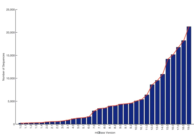
mi-croRNAs is very important for biologists. As of August 2012, 21,264 mature microRNAs
have been identified in miRBase [17], which is a biological database that acts as an archive
of microRNA sequences and annotations. Figure 1.1 shows the number of microRNA
se-quences which are published in different releases of miRBasedatabase. Although a large
number of microRNA sequences have been identified, a vast number of them are yet to be
identified. This rapid growing is due to the different approaches which have been proposed
for identifying these tiny molecules in recent years.
Initially, the only techniques for identifying microRNAs were experimental methods.
Experimental methods use DNA cloning for microRNA identification. However, these
methods suffer from low performance because of environmental conditions and low level
expression of microRNAs. As an alternative, computational methods can discover
microR-NAs without conducting any experiment in wet laboratories. The main signal in identifying
microRNAs is the hairpin secondary structure of the precursor microRNA (pre-microRNA).
Computational methods rely on this fact for distinguishing these tiny molecules from other
types of sequences.
Dozens of methods have been proposed in recent years, especially after 2005, which
propose approaches for identifying microRNAs and many of these methods have acceptable
performance. However, the database that they are using in training and testing process is not
representative of the whole genome, and classifiers are built on a not-so-complete dataset.
In addition, many of the proposed methods use a large number of features and they do
not select a subset of features for reducing the complexity of the classifier as well as a
road for biologist to interpret the limited number of features in the feature subset. Thus,
0 5,000 10,000 15,000 20,000 25,000
mi Base Version
N u mb e r o f Se q u e n ce s 1
.0 1.1 1.2 1.3 1.4 .02 2.1 2.2 3.0 3.1 4.0 5.0 5.1 6.0 7.0 7.1 .08 8.1 8.2 9.0 9.1 9.2
1 0 .0 1 0 .1 1 1 .0 1 2 .0 1 3 .0 1 4 .0 1 5 .0 1 6 .0 1 7 .0 1 8 .0 1 9 .0
Figure 1.1: MiRBase database growth between December 2002 and August 2012.
work, a dataset is selected which both pseudo hairpins and other types of non-coding RNA
sequences.
On the other hand, LDR methods are well-known and well-studied classifiers in
ma-chine learning and pattern recognition. These methods have shown very good performance
in various applications. However, at this time there is no microRNA identification approach
which is built based on based classifiers. In addition, the performance of the
LDR-based classifier can be enhanced further by explicitly mapping the data to higher
dimen-sional space, which again, at this time, have never been proposed to use with LDA-based
classifiers. In addition, the feature selection algorithm that is chosen is based on wrapper
methods which have advantages over filter methods in the sense that they uses the classifier
itself for evaluating the performance comparing to using some evaluation metrics regardless
1.4
Problem
In this thesis, the problem that is being tackled is:
Distinguishing microRNA precursor sequences from non microRNA
pre-cursors, pseudo hairpins and other non-coding RNAs sequences.
1.5
Contributions
The main contributions of this thesis are:
• Proposing a new classification scheme that combines LDR classification methods and
microRNA features.
• Comparison of using explicitly mapped data fed into the classifier and using the
orig-inal data. These methods have never been used with LDR classifiers.
• Utilizing feature selection algorithm for selecting fewer features.
• Designing and implementing a framework for automating and handling a large
num-ber of experiments and using a database server for storing the results.
In this thesis, we focus on identifying human pre-microRNAs from other molecules
which are not human pre-microRNA. There are many methods available for this purpose
but none have ever utilized the well-known LDR classifiers. In addition, I use wrapper
feature selection methods for selecting a representative feature subset. In addition, the idea
of mapping the data to higher dimensions in an explicit form have never been used in LDA
1.6
Thesis Organization
This thesis has six chapters. Chapter II presents information about microRNAs and
differ-ent approaches which were introduced previously. Chapter III provides the required
back-ground about different pattern recognition concepts used in this research work. Chapter IV
describes the proposed model, the dataset and the features which are used. In Chapter V,
experimental results are presented and a comparison has been made with previously
pro-posed methods as well as a discussion about the results. Finally, in Chapter VI, conclusions
MicroRNAs
2.1
Gene Expression
Thecentral dogma of molecular biologydescribes the way in which genetic information
is transferred from DNAs to proteins: that is DNA→RNA→Protein (see Figure 2.1) [24].
The first process is calledtranscriptionin which an RNA molecule is synthesized from the
information included in a section of DNA. The RNA molecule which is produced is called
Messenger RNA (mRNA). The other process in which the protein molecule is produced
from the mRNA is calledtranslation.
Activation of an organism’s genes depend on the cell’s environment and needs of the
cell in addition to the fact that genes might be expressed at different times. There are
different mechanisms of gene regulation inProkaryoticsandEukaryotics. However, one of
RNA Transcription
DNA Translation Protein
Figure 2.1: The central dogma of molecular biology.
the most important mechanisms is thetranscriptional regulation. An enzyme called, RNA
polymerase is responsible for the transcription regulation [24].
In addition to transcriptional regulation, gene regulation can be done at another step
after transcription on the mRNA in a process called post-transcriptional process. A novel
mechanism of gene regulation that happens after the transcription process is by tiny molecules
calledmicroRNAs(miRNA) [3].
2.2
MicroRNA
MicroRNAs are a large class of small non-coding RNAs that have post-transcriptional gene
regulatory roles. The first two microRNAs that were discovered are lin-4 and let-7 of
Caenorhabditis elegans [24]. It has been shown that these two microRNAs are involed
in controlling the timing of larval development.
2.3
Biogenesis of MicroRNA
These tiny molecules repress translation of messenger RNAs (mRNA) into proteins in one
of the two ways based on the complementarity level between the microRNA and their
tar-gets by binding into mRNAs. In the first method, microRNAs bind perfectly or almost
perfectly to mRNA sequences and cause their cleavage by multiprotein
RNA-induced-silencing complex (miRISC). This event causes degradation of the target mRNA. This
mechanism of miRNA-mediated gene silencing can usually be found in plants, and in rare
cases occurs in animals. However, in most animals, microRNA sequences use another
mechanism for regulating the genes which does not lead to target mRNA’s cleavage. These
0 1 A U G C U U C C G G C C U G U U C C C U G A G A C C U C A A G U G U G A G U G U A C U A U U G A U G C U U C A C A CC U G G GC U C U CC G G G U A C C A G GA C G GUU
U G A G C AG A U
Figure 2.3: The biogenesis of microRNAs. Figure is taken from [12] by authors’ permis-sion.
UTR) of target mRNAs and repress the translation process of mRNAs into proteins. This is
done through a RISC complex which is identical or highly similar to the one that is used in
the first mechanism.
Since 2004, the biogenesis of miRNAs has been elucidated (Figure 2.3). Initially,
mi-croRNAs are transcribed by RNA polymerase II in nucleus as large RNA precursors that
are called primary microRNAs (pri-microRNA) and are capped (MGpppG) and
polyadeny-lated (AAAAA) [12]. In nucleus, pri-microRNA is processed by an enzyme called Drosha,
and the double-stranded-RNA-binding protein, Pasha. A 70-nucleotide sequence called
pre-microRNA is the product of this step which folds imperfectly into a hairpin secondary
and exportin 5. After that, another enzyme known as Dicer, cuts the loop and generates
a double-stranded RNA of about 22-nucleotides in length known as miRNA:miRNA*
du-plex. The duplex is detached and then one of the strands binds into miRISC comdu-plex. The
mature microRNA strand that is incorporated miRISC complex can be used to negatively
regulate its target genes [12].
2.4
MicroRNA Identification
Earlier, microRNAs were only identified by using experimental methods. The traditional
experimental approaches to microRNA discovery are cloning and sequencing [10], and can
detect novel microRNAs. Since microRNAs are usually expressed at low levels and depend
on tissue and conditions of the cell, these methods may be unable to identify new
microR-NAs [3]. Recently high-throughput sequencing approaches, in particular, 454 sequencing,
have become popular for discovering new microRNAs [13].
Another category of approaches for identifying microRNAs is computational methods.
The main idea behind these methods is to analyze hairpin secondary structures of precursor
microRNAs (pre-microRNA). Secondary structure of pre-microRNA allows researchers to
propose computational methods that can distinguish these sequences from other sequences
in the genome. The currently proposed computational methods for identifying microRNAs
have been developed in two directions, comparative methods and non-comparative
meth-ods.
Comparative methods have been developed based on the study that shows microRNAs
are highly conserved in related genomes [3]. Therefore, some methods use this property of
microRNAs and introduce candidate microRNAs which fold into hairpin secondary
The other direction of computational methods does not rely on conservation characteristics
of microRNAs. These methods are mainly based on effective and efficient identification of
microRNA among all other sequences which share similar secondary structure as
pre-microRNA. As mentioned earlier, pre-microRNAs fold into stem-loop secondary structure.
There are a few challenges which should be mentioned. The first one is that, there are
thousands of other genome sequences which fold into hairpin secondary structure, called
“pseudo hairpins” [5]. Second, many of other non-coding RNAs such as YRNAs,
snR-NAs and tRsnR-NAs fold into hairpin secondary structure as well. Therefore, the challenges are
extracting set of features from sequences for forming a representative dataset and then
ap-plying a classification method that effectively identifies and distinguishes pre-microRNAs
from other non-coding RNAs and pseudo hairpins.
In this research work, the focus is on developing a computational method for identifying
pre-microRNAs based on approaches that do not rely on conservation information
(non-comparative methods). In Section 2.5, many of these methods are reviewed.
2.5
Related Works
The idea of identifying microRNAs without relying on phylogenetic knowledge about the
genome started with the works of [28], [34] and [39] and they all exerted great influences
on the identifying microRNAs problem. Since 2005, many papers have been published
in journals and conference proceedings and each of those made a contribution toward
ef-fectively identifying microRNAs. All papers in this area can be categorized based on the
classification approach they have adopted and also based on the features they have
intro-duced and employed for classification. There is a large degree of overlapping between the
defining a clear boundary between different approaches based on features and classification
algorithms seems unfeasible. Therefore, in this work, papers have been introduced in a
chronological order.
2.5.1
Focusing on Genome Regions Around Known MicroRNAs
Studies indicate that the total number of microRNA genes is larger than what had been
iden-tified prior to 2005. Therefore, microRNA gene discovery remained an important task in
this field for understanding unknown regulation mechanisms. In particular, computational
approaches had been found to be very useful for guiding experimental analysis. Then Sewer
et al.[34] introduced a method for tackling this problem and called itmiRabela.
In their work, the authors only focused on regions of the genome where known
microR-NAs had already been found. Then extracted sequences which can fold into stem-loops and
have a robust secondary structure. The authors proposed 40 new features for characterizing
sequential and secondary structure properties in relation to previously discovered
microR-NAs as well as negative samples as the input of the classification algorithm. They employed
support vector machines for doing the classification. At the end, for guiding experimental
investigations, the authors also developed a probabilistic statistical model which estimates
the number of pre-microRNAs in a given genomic sequence.
Seweret al. [34] used a dataset containing 178 positive samples as well as 5,395
neg-ative samples for classification. Positive samples were taken from the humanRfam
reposi-tory. Negative samples are random sequence samples from tRNA, rRNA and mRNA.
Seweret al.[34] claim that the model they have developed, recovers 71% of the positive
pre-microRNA sequences with false positive rate of 3% and false negative rate of 29%.
addition, it is stated that the method can successfully identify microRNAs that are missed
by previously developed methods.
2.5.2
Local Contiguous Structure-sequence Information of Stem-loops
Xueet al. [39] also felt the need for a method which can discern pre-microRNAs from other
segments of sequences with similar hairpin structure (pseudo pre-microRNAs) and which
does not rely on comparison with known microRNAs. Developing such methods is of some
importance both for gaining more information about microRNAs and for identifying new
microRNAs without comparing with previously discovered microRNAs. Xue et al.
pro-posed 32 new triplet element features of “local contiguous structure-sequence information
of stem-loops” for differentiating pre-microRNAs from pseudo pre-microRNAs.
For classification experiments, one training and two testing datasets were built and
sup-port vector machines (SVM) was used as the classification method. The training dataset,
which was called TR–C, contained 163 and 168 human microRNAs and pseudo
microRNAs, respectively. The first test dataset, called TE–C, included 30 human
pre-microRNAs which did not overlap samples from TR-C and 1,000 pseudo pre-microRNAs.
The second test dataset, called CONSERVED–HAIRPIN, contained 2,444 pseudo
pre-microRNAs. Also the authors applied the classifier on 581 pre-microRNAs from 11 species
other than human and called this dataset CROSS-SPECIES. They noted that pre-microRNAs
with multiple loops had been filtered out from the datasets. In addition, they conducted an
analysis on the “discriminant power of the different triplet elements”.
Xueet al. claim that, their SVM classifier on the TE-C dataset, successfully classified
28 out of 30 human pre-microRNAs and 881 out of 1,000 pseudo pre-microRNAs, which
on the CONSERVED-HAIRPIN dataset, the classifier detected 2,174 out of 2,444 pseudo
pre-microRNAs which gives a specificity of 89.0%. On the CROSS-SPECIES dataset, they
claim that the classifier identified 90.9% of pre-microRNAs. In addition, they claim that
due to high accuracy, pre-microRNAs and pseudo pre-microRNAs are distinct with respect
to proposed triplet element features, despite the fact that they have similar hairpin structure.
They also assert that the classifier is also capable of identifying microRNAs of other species
rather than human even though it was trained with human pre-microRNAs and shows the
proposed features might reflect a quality which is same for all species.
2.5.3
One-class Compared Two-class Classifiers
Machine learning algorithms which do not rely on defining the negative class and only
depend on the positive class have been getting more attention from researchers in
bioin-formatics. That is because generation of the negative class might be problematic and not
representative enough. Yousefet al.[40] used a one-class approach for finding microRNAs.
The authors criticize previously proposed approaches for relying on generation of an
artificial negative class since if the negative class is not generated properly, performance
estimation of the classifier might be biased and/or reduce the classification performance
significantly.
Yousef et al. propose a method which only uses putative microRNAs as the positive
class for the training procedure and does not need a negative class. The one-class approach
only needs microRNA sequences for building the model. In addition, the authors propose 62
features which are extracted from both secondary structure and sequence of the microRNAs.
The authors conducted many experiments for evaluating and comparing the
They performed experiments on the following pre-microRNA datasets: human, mouse,
C.elegans. The following classification methods were also used: one-class SVM, one-class
Gaussian, one-class PCA, one-class KNN, two-class na¨ıve Bayes and two-class SVM.
Au-thors also conducted an experiment on finding microRNA genes in theEpstein Barr Virus
(EBV)genome.
Yousef et al. state that results of one-class approaches for Gaussian and KNN show
slightly better performance. Whereas on average accuracy of one-class approaches are
around 8% to 10% lower than two-class methods. Authors claim that applying the method
on EBV genome showed that all one-class approaches could distinguish EBV microRNAs
with sensitivity of 72% – 90% in which one-class PCA has the highest sensitivity.
Yousefet al. [40] claim that their newly introduced features can describe microRNAs
more accurately than previously proposed features. Also, it is stated that the one-class
method is very useful especially when negative samples are not clearly defined which is
usually true when a new organism is being analyzed.
2.5.4
Global and Intrinsic Folding Features
Identifying microRNAs from a pool of sequences without sacrificing putative microRNAs
is a very challenging task. That is because microRNAs are relatively short in length and
“have highly diverse base compositions”. Ng and Mishra [29] propose a method for
tack-ling this problem. The authors criticize the approach proposed in [39] in which they are
limited to only microRNAs without multiple loops. They point out low sensitivity of [28]’s
approach that is 73%. Authors also state that the approach presented in [41] rely on
com-parative analysis of results in order to reduce the false positive rate. In addition, they state
the features which are used in the referred approaches.
Ng and Mishra [29] propose 29 new “RNA global and intrinsic folding” features and
employ SVM as the classification algorithm. Features can be categorized as follows:
se-quential, hairpin folding-related, statistical thermodynamics and topological. The authors
refer to their classifier asmiPred.
The authors obtained a total number of 2,241 pre-microRNAs from miRBase 8.2. They
used 200 humanpre-microRNAs and 400 randomly selected pseudo hairpins for training
and finding parameters ofmiPredand called it TR-H. Another dataset containing 123
hu-manand 246 pseudo hairpins were used in the testing procedure, which is referred to as
TE-H. The authors also evaluated performance of themiPredon three other datasets from
non-human species, ncRNAs and mRNAs which are referred to as NH, NC and
IE-M, respectively. In addition, they experimented screening viral-encoded microRNA genes
using four complete viral genomes. Finally, an analysis of contribution of each and
ev-ery feature to miPred classification ability was done to see whether selecting a subset of
features leads to improvement or worsening the performance of the classifier.
Ng and Mishra [29] claim that, they achieved 88.00% / 97.50% / 94.33% and 84.55%
/ 97.97 % / 93.50% which are sensitivity(SE), specificity (SP) and accuracy (ACC) for
TR-H and TE-H, respectively. And, the authors state that miPred can achieve 87.65%
/ 97.75% / 94.38% for SE/SP/ACC when it was used on the IE-NH dataset. Applying
the classifier on IE-NC and IE-M led to performance specificity of 76.15% and 87.10%,
respectively. As for viral genome, the classifier can classify microRNAs with sensitivity
and specificity of 100.00% and 93.75%, respectively. They claim that investigation on
importance of the features in terms of discriminant power, shows that all the features are
power among all other features.
Ng and Mishra also claim that their approach has “comparable or significantly” better
identification performance when comparing it to all previously proposed methods. They
also suggest usingmiPredas a tool for experimental research.
2.5.5
Enhancing Global and Intrinsic Folding Features
MicroRNAs are an important type of non-coding RNAs which participate in
post-transcrip-tional gene regulations. It is well studied that, there is an association between microRNA
expression levels and many diseases. Therefore, Batuwita and Palade [4] believe that it
is very important to provide a computational tool for biologists to be able to effectively
identify microRNA genes in genomes. Thus, they introduced a model for microRNA
iden-tification.
Batuwita and Palade criticize previous works for only relying on genome pseudo
hair-pins for generating the negative class. However, they state that there are vast number of
sequences which fold into hairpin secondary structure and are non-coding RNAs
(ncR-NAs). Although they mentioned that the authors of [34] considered tRNAs and rRNAs in
the negative training dataset, and the dataset was not representative enough.
The authors introduce a new negative dataset containing other ncRNAs and genome
pseudo hairpins and state that the dataset is “complete and representative”. They also
propose a new set of features, used feature selection algorithms and tried to solve
class-imbalance problem.
The authors performed some experiments on a dataset containing 691 human pre-microRNA
sequences in the positive class and 9,248 false pre-microRNAs in the negative class. They
performed experiments for finding the best subset of features and for tackling the
class-imbalance problem which they say it arises when the number of samples in the positive
class and the negative class is highly unbalanced. Finally, they applied their method on a
dataset containing pre-microRNAs across 49 and 12 animals and viruses, respectively.
Batuwita and Palade [4] state that their method achieved 80.23% / 98.71% / 89.04%
forSE/SP/Gmwhen using all features. Applying feature selection algorithms resulted in a
subset of features containing 21 features instead of all 48 features with 83.36% / 99.00% /
90.84% forSE/SP/Gm. It is shown that the class imbalance learning results are as follows:
90.02% / 97.28% / 93.58% forSE/SP/Gm. Finally, applying the proposed method on
non-human datasets showed accurate microRNA prediction. The authors [4] claim that, their
method has better performance by comparing it to previous methods. In addition, they claim
that their method could be coupled with deep-sequencing data to incorporate advanced
features introduced in those methods.
2.5.6
Co-learning of Sequence and Structure
Namet al.[28]’s approach mainly relies on a hidden Markov model for identification of
mi-croRNAs. Identification of microRNA genes is a very important problem for understanding
post-transcriptional gene regulation. Computational approaches for identifying microRNAs
could be used even when microRNA is expressed low or in a particular tissue.
Namet al.propose a probabilistic co-learning approach that is based on a paired hidden
Markov model (HMM) for identification of microRNAs while continuously considering
structure and sequence of pre-microRNAs. In Namet al. method [28], each pre-microRNA
is represented as a pairwise sequence which can be modeled as a sequence of matched
each position of the pairwise sequence has two states, structural and hidden.
A dataset consisting of 136 human pre-microRNAs in positive class and 1,000
ran-domly selected pseudo hairpins as negative, was used during the experiments. The
au-thors performed some experiments on the positive and negative datasets using 5-fold
cross-validation, and ROC curves were also plotted for analyzing the performance. They also
used the method for scanning human chromosomes 16, 17, 18 and 19 for detecting
pre-microRNA candidates.
Namet al.state that on average the method successfully classified pre-microRNAs with
72.8% sensitivity and 95.9% specificity. The method was able to detect 253, 274, 83 and
207 pre-microRNA candidates on chromosomes 16, 17, 18 and 19, respectively.
2.5.7
The Ranking Algorithm Based on Random Walks
These are some of the reasons why Xu et al. [38] introduced a new method for solving
this problem. They noted that previous works were not effective on regions of genome
which are not annotated very well and this is because obtaining a set of negative examples
is difficult. In addition, they comment on lack of positive examples in many species except
in well studied species, such asA.gambiae.
Xuet al.proposed a ranking algorithm which is based on random walks. The approach
tries to find new microRNAs in genomes even when only a few number of microRNAs
are known and the genome is annotated poorly. It is stated that the algorithm requires no
negative samples. Basically, the authors formulate identifying microRNAs as an
informa-tion retrieval problem in which microRNAs should be retrieved from a set of microRNA
candidates. Each sample is represented as a vector containing 36 features. Among these
fea-tures are as follows: “normalized free energy of folding (MFE)”, “normalized base-pairing
propensities” of both strands of the pre-microRNA and “normalized loop length”.
Xuet al. [38] performed experiments onH.sapiensandA.gambiae(533 and 38,
respec-tively). Also, they generated other sequences fromH.sapiensandA.gambiaegenomes for
making a pool of sequences. They evaluated performance of the method on the two
men-tioned datasets. The authors also conducted an analysis on conservation of theA.gambiae.
They claim that their method achieved accuracy higher than 95.00% on putative
hu-man microRNAs, and in theA.gambiae experiment, the algorithm could correctly predict
200 microRNAs. Also, conservation analysis revealed that 78 out of 200 microRNAs are
conserved in at least one other animal species.
In addition, the authors claim that their method can be applied on newly sequenced
genomes in which full annotation has not been done. They also state that it does not rely
on conservation between species. Thus, they believe that their method can be used as a
powerful tool for prediction of novel microRNAs in viral genomes.
2.5.8
The Na¨ıve Bayes Algorithm
Yousefet al.[41] refer to the work ofNam et al.[28] and state that they also used features of
microRNA genes instead of relying on conservation of microRNAs between related species.
The authors pointed out that Namet al. [28] only used human microRNAs and a limited
set of negative samples for training and testing. In addition, the approach proposed in [28] is
a very specific probabilistic model which uses prior knowledge for constructing the model
and defining the states.
Yousefet al. [41] described a new approach that is based on the na¨ıve Bayes classifier.
classi-fier and analyzer for selecting the sequences with highest probability of being a microRNA.
The classifier is built using a dataset consisting of sequential and structural features of
pu-tative microRNAs from multiple species. Finally, the model uses a comparative analysis to
reduce the number of false positive potential microRNAs. The authors state that the novelty
of the work is in using a variety of organisms for building the model.
The authors state that their various experiments were conducted for evaluating the
per-formance of the model. First, the training process was applied to microRNAs ofC.elegans
and Mouse. Experiments were done with different sizes of negative sample sets.
Eval-uation was followed by 5-fold cross validation and the receiver operating characteristic
(ROC) curve. After single species, the learning procedure was done with microRNAs from
multiple organisms with the same training and evaluating methods used in single species
step. Finally, an experiment was conducted for predicting microRNA genes in theMouse
genome.
The authors claim that their model can achieve specificity and sensitivity of 96% and
83% forC.elegansand 91% and 97% forMouse, respectively. For multiple species
exper-iments, they claim that their model can successfully classify the data with high accuracy.
Finally, they stated that the model detected a reasonable number of microRNA genes.
The authors claim that their model has a high generalization ability since it is trained
using microRNAs of multiple organisms. Thus, they state that this method can be used for
identifying microRNAs in a wide range ofEukaryotes. Also, they state that their algorithm
can achieve higher specificity and similar sensitivity compared to all previously developed
2.5.9
The Random Forest Algorithm For Classification
Jianget al.[21] proposed a method called MiPred for distinguishing pre-microRNAs from
other sequences with similar stem-loop secondary structure. Identifying pre-microRNAs
systematically and experimentally tend to miss novel pre-microRNAs and is highly
de-pendent on cell’s condition. That is why computational approaches which do not rely on
comparative genomic-based method play very important roles.
The authors propose a method that uses a set of 34 features including minimum free
energy (MFE) of the secondary structure, “local contiguous triplet structure composition”
andP-value of randomization test. All these features are then given to a machine learning
algorithm, called random forest (RF) [21].
Jiang et al. [21] state that they used a dataset containing human pre-microRNAs and
human pseudo hairpins for training and testing the classifier while using different features.
Then after training and testing they used SVM instead of random forest to evaluate
dis-tinctive power of the proposed features regardless of the classifier algorithm. The homo
sapiensdataset contained 462 human pre-microRNA whereas the pseudo pre-microRNA
dataset contained 8,494 pre-microRNA-like hairpins. The authors also conducted an
anal-ysis on the importance of the features in order to rank features based on their prediction
performance throughout the training procedure. In addition, they also implemented at-test
for comparing the performance of random forest and SVM.
The authors state that their classifier predicts pre-microRNAs while using all features
(local contiguous, MFE and P-value of randomization test with 90.47%/95.09%/96.68%
specificity / sensitivity / accuracy. Also, the classifier achieves its lowest performance when
it uses contiguous features. Jianget al. [21] state that the SVM classifier with the same set
They claim that on average SVM is about 0.50% lower than RF with p-value of 0.003.
Finally, the authors claim that analyzing importance of the features show thatp-value and
MFE are the two most influential features among all other features.
The authors claim that minimum free energy andp-value of randomization test are very
important features which can be used in identifying pre-microRNAs when random forest is
used as the classifier.
2.5.10
Structural Motifs
Brameier and Wiuf [6] propose a method for distinguishing microRNAs by genome
scan-ning which only depends on secondary structure of pre-microRNAs from pseudo hairpins.
The proposed classifier relies on linear genetic programming which contains “multiple
reg-ular expressions (motifs)” matched to pre-microRNAs secondary structure. The authors
also propose a new criterion for selecting potential microRNA candidates.
The authors used 474 human pre-microRNAs from miRBase 9.0 for the positive set
and 100,000 sequences, which were taken from 20,000 random locations in the human
genome, for the negative set. After pre-filtering the two datasets, the authors used datasets
for training the motif-based classifier and tried with 16 different motifs. An ROC curve was
used for comparing the performance when using different numbers of motifs. In another
experiment, the authors applied 5-fold cross-validation to evaluate the classification
perfor-mance. In addition, other experiments were performed which are as follows: evaluating the
performance on other species, scanning human genome for finding new microRNAs.
Brameier and Wiuf [6] claim that they achieved 99.90% / 87.00% and 99.10% / 95.00%
for sensitivity and specificity when using 16 motifs and 1 motif, respectively. In 5-fold
sensi-tivity during training and testing, respectively, whereas on average, specificity remained at
99.10%. Also, the authors claim that their method predicts 74% and 81% percent of mouse
and rat microRNAs when using all motifs. However, it identified 91 and 98 percent when
using half of the motifs. It was stated that scanning human genome resulted in identifying
117 new microRNAs on human chromosome 19.
Brameier and Wiuf [6] claim that their method is competitive when compared to all
previously developed approaches. Also, they state that their method requires less amount
of knowledge about pre-microRNAs. In addition, using motifs and genetic programming
enhances knowledge interpretation and extraction.
2.5.11
The Kernel Density Estimation Algorithm
Changet al. [8] proposed a method for identifying microRNAs. They believe that having
a computational approach which does not rely on analyzing the similarity of the sequence
with putative microRNAs, and can work without prior knowledge about microRNA
homol-ogy, is necessary. They focus on a classification methodology for microRNA identification
and use the relaxed variable kernel density estimator (RVKDE) which is an instance-based
classification algorithm. The authors use 40 features which were all previously introduced
in other works.
Chang et al. [8] conducted some experiments for evaluating the performance of the
classifier. They used a dataset containing 400 human pre-microRNAs (HU400) and they
used 5-fold cross-validation for measuring the performance as well as comparing it with
previous methods. Then, they used the trained classifier for extending the experiment to
non-human microRNAs. The dataset they used for this experiment includes 1,675
using the RVKDE on the performance of the classifier. Finally, they performed an
experi-ment for explaining characteristics of the RVKDE in microRNA prediction.
The authors state that their classifier can achieve 90.5% / 97.5% / 94.0% of SE / SP
/ ACC on HU400 dataset. Sensitivity, specificity and accuracy of the RVKDE classifier
are 96.7%±2.7%, 93.9%±2.1% and 95.3%±1.4%. The authors state that investigating the
effect of using RVKDE revealed that its performance is identical or better than SVM and
also it tends to maximize specificity, whereas SVM tries to maximize sensitivity. At the
end, Changet al. [8] state that the RVKDE is “instance based and highly dependent on the
local information” of training samples.
The authors claim that theRVKDE is more suitable for microRNA identification since
it uses more local information about the sequences. On the whole, the authors believe
that good performance of their classifier should encourage more research on classification
methods and feature extraction.
2.5.12
Feature Selection via a
Genetic Algorithm
As noted earlier, identification of microRNAs play a crucial role in understanding their
biological functions in cells and can potentially lead to curing many diseases. There are
plenty of methods and dozens of features proposed for distinguishing these tiny molecules.
However, selecting a subset of features which can help biologists to interpret them is very
important. Thus, Wanget al. [36] propose a feature selection method that is based on a
genetic algorithm (GA) for selecting the best subset of features.
Wanget al.[36] refer to microPred [4] in which they use afilterbased feature selection
method. However, it has been shown that the performance of wrapper feature selection
uses a GA-based algorithm to optimize the feature subset of an SVM classifier.
Wanget al.[36] use the dataset which was used in [4]. They use 183 features extracted
from literature for the original feature set. The authors use the accuracy of five fold
cross-validation of SVM classifier as the fitness function of the GA algorithm. They use many
performance metrics in their work such as accuracy, specificity, sensitivity, F-measure and
Matthews correlation coefficient for evaluating the performance.
Wanget al. [36] claim that their proposed classifier recognized 13 features as the best
subset of features and it achieved anaccuracyof 93.97% which is higher than that of
micro-Pred and mimicro-Pred. At the end, they also used their classifier on the most recently published
microRNA dataset and the authors claim that the performance was satisfactory.
2.5.13
Sample Selection for Classification
As noted in many previous methods, class imbalance is one of the problems which should be
considered when designing a classifier for microRNA identification. Han [20] proposed an
approach which only focuses on solving the class imbalance problem. The author believes
that an unbalanced dataset should be first manipulated in order to reduce the negative effects
of the unbalanced data.
As mentioned earlier, the imbalance problem arises since the number of samples in
the negative class outnumbers samples in the positive class. Han [20] proposed a method
which reduces the number of samples in the negative class by clustering methods. Thus,
he proposed to cluster positive and negative training samples based on their stem similarity
and their distribution in high dimensional sample space, respectively. This approach results
in having a dataset which is quite balanced and can be used for classification. The author
Han [20] claims that the proposed approach is around 12% more accurate than
micro-Predwhich means that it can achieve a performance of nearly 100%. The result the author
claims is surprisingly good and the way it is described all the microRNA precursors can be
classified accurately from non pre-microRNA sequences. However, further analysis should
be done in order to guarantee that reducing the number of samples in this way will not
Dimensionality Reduction and Explicit
Mapping
Pattern recognition is a research area that has attracted many researchers. It is mostly an
interdisciplinary field of study covering computer science, statistics, engineering, artificial
intelligence and many other subjects. It has been widely used in different applications such
as classifying cancerous genes, identifying spam emails, image recognition and credit card
fraud detection [11]. In recent years, significant progress has been made specially where
the research domain overlaps with probability and statistics and many improvements have
been achieved both in application side as well as in methodology.
A particular active area of pattern recognition is the application of algorithms and
tech-niques in solving bioinformatics problems. Analyzing large biological datasets requires
employing pattern recognition and machine learning techniques in order to extract useful
knowledge out of them. Examples of application of this field in bioinformatics include
iden-tifying clusters of gene expression data, distinguishing different types of protein-protein
interactions, cancer classification based on microarray data and many others. Therefore,
pattern recognition methods have been well used in bioinformatics problems.
3.1
Dimensionality Reduction
The complexity of the most learning algorithms relies on the number of input dimensions,d
and number of input data samples,N. For reducing the complexity, decreasing the number
of dimensions of the input data is desirable. In addition, simpler models are more robust
and less dependent on noise and outliers. Also, when fewer dimensions are used in learning
methods without loss of relevant information, data can be visually analyzed and interpreted
[2].
Generally, there are two methods for reducing the dimensionality of learning systems
feature selection and feature extraction [2]. Infeature selectionmethods, the goal is to select
kof theddimensions (features) of the dataset that can be representative of the classes and
can give the most information about the original dataset. Oncek dimensions are selected,
the otherk−d dimensions will be ignored and considered useless.
Infeature extractionmethods, it is desired to find a set ofkdimensions, which are
com-binations of original features. Depending on whether we use the class labels of the samples
or not, these methods are categorized intosupervised andunsupervised. Well-known
fea-ture extraction methods arePrinciple Component Analysis andLinear Discriminant
Anal-ysis(LDA) which are unsupervised and supervised algorithms, respectively. In this study,
3.1.1
Linear Discriminant Analysis
Linear discriminant analysis (LDA) is a supervised approach for dimensionality reduction
for classification problems originally developed by R.A. Fisher in 1936. LDA is a
well-studied topic in pattern recognition. This is one of the methods available for linear
di-mension reduction. The advantage of using a linear transformation is that, although the
derivation of the underlying transformation may be slower, the classification is extremely
fast as it performs linear-time operations to reduce the dimensions, typically, much lower
than the original one. There are different schemes for finding transformation matrix A
which can project the data into lower dimensions in a way what the new classes are as
sep-arate as possible while classes are as compact as possible. In this work, we consider three
different LDA schemes; the well-know Fisher’s discriminant analysis (FDA) [11, 14], the
heteroscedastic discriminant analysis (HDA) approach [25], and the Chernoff discriminant
analysis (CDA) approach [33]. All these three methods propose different approaches for
finding a “good” transformation matrix A. A brief discussion of these three schemes is
given in the next three sections.
We consider two classes, ω1 and ω2 (positive and negative classes), represented by two normally distributed random vectorsx1∼N(m1,S1)andx2∼N(m2,S2), respectively,
withp1andp2the a priori probabilities. After the LDA is applied, two new random vectors
y1=Ax1 andy2=Ax2, where y1∼N(Am1; AS1At)andy2∼N(Am2; AS2At)withmi
andSibeing the mean vectors and covariance matrices in the original space, respectively.
The aim of LDA is to find a linear transformation matrix A in such a way that the new
3.1.1.1 Fisher’s Discriminant Analysis
LetSW = p1S1+p2S2 andSE = (m1−m2)(m1−m2)t be the within-class and
between-class scatter matrices respectively. The well-known FDA criterion consists of maximizing
the Mahalanobis distance between the transformed distributions by finding A that
maxi-mizes the following function [11]:
JFDA(A) =tr {
(ASWAt)−1(ASEAt) }
. (3.1)
The matrixAthat maximizes (3.1) is obtained by finding the eigenvalue decomposition of
the matrix:
SFDA=SW−1SE, (3.2)
and taking thed eigenvectors whose eigenvalues are the largest ones. SinceSE is of rank
one,SW−1SE is also of rank one. Thus, the eigenvalue decomposition ofSW−1SE leads to only
one non-zero eigenvalue, and hence FDA can only reduce to dimensiond=1.
3.1.1.2 Heteroscedastic Discriminant Analysis
HDA was proposed as a new LDA technique for normally distributed classes [25], which
takes the Chernoff distance in the original space into consideration to minimize the error
rate in the transformed space. It can be seen as a generalization of FDA to consider
het-eroscedastic classes, and the aim is to obtain the matrixAthat maximizes the function:
JHDA(A) =tr {
(ASWAt)−1[ASEAt
−AS 1 2 W
p1log(S−
1 2 W S1S
−1 2
W )+p2log(S −1
2 W S2S
−1 2 W )
p1p2 S
1 2 WAt
]}
where the logarithm of a matrixM, log(M), is defined as:
log(M),Φlog(Λ)Φ−1. (3.4)
withΦandΛrepresenting the eigenvectors and eigenvalues ofM, respectively.
The solution to this criterion is given by computing the eigenvalue decomposition of:
SHDA=SW−1 [
SE−S 1 2 W
p1log(S−
1 2 W S1S
−1 2
W )+p2log(S −1
2 W S2S
−1 2 W )
p1p2 S
1 2 W
]
(3.5)
and choosing thedeigenvectors whose corresponding eigenvalues are the largest ones.
3.1.1.3 Chernoff Discriminant Analysis
CDA is an LDA method that has been recently proposed, and its aim is to maximize the
separability of the distributions in the transformed space, measured by the Chernoff distance
between the two classes. CDA assumes that the classes are normally distributed (in the
original and transformed spaces), maximizing the following function [33]:
JCDA(A) =tr{p1p2ASEAt(ASWAt)−1
+log(ASWAt)−p1log(AS1At)−p2log(AS2At)}
(3.6)
whereSW = p1S1+p2S2,SE = (m1−m2)(m1−m2)t.
It has been shown in [33] that for any normally distributed random vectors,x1 andx2,
there always exists an orthogonal matrixQ, whereQQt=I, such thatJCDA(A) =JCDA(Q)
for any matrixAor rankd. Thus, without loss of generality, here, we assume thatAis an
function (3.6) in an iterative way. The algorithm starts with an arbitrary orthogonal matrix
A(1), and at stepk+1,A(k+1) is computed as follows:
A(k+1)=A(k)+αk∇JCDA(A(k)) (3.7)
where the gradient forJCDAis:
∂JCDA
∂A =∇JCDA(A) =2p1p2
[
SEAt(ASWAt)−1
−SWAt(ASWAt)−1(ASEAt)(ASWAt)−1 ]t
+2[SWAt(ASWAt)−1−p1S1At(AS1At)−1
−p2S2At(AS2At)−1
]t
For this gradient algorithm, a learning rate, αk needs to be computed. In order to ensure that the gradient algorithm converges,αkneeds to be maximized. In [33], the secant method is used for this, and the aim is to maximize the function:
ϕk(α) =JCDA(A(k)+α∇JCDA(A(k))) (3.8)
Starting with two initial valuesα(0) andα(1), the value ofα(j+1) at time j+1 is iteratively found as follows:
α(j+1)=α(j)+ α(j)−α(j−1) dϕk
dα(α(j))− dϕk
dα(α(j−1)) dϕk
dα(α
(j)) (3.9)
where
dϕk
dα(α) = [∇JCDA(A (k)
+α∇JCDA(A(k)))]·∇JCDA(A(k)) (3.10)
matricesCandD, as follows:C·D=tr{C D}. The value of∇JCDA(A(k)+α∇JCDA(A(k))) is computed by replacingAbyA+α∇JCDA(A)in the Equation (3.8).
Finally, with the definition of dϕk
dα(α), Equation (3.9) can be solved, and the gradient algorithm continues with the next iteration. The complete algorithm can be found in [33].
One of the keys in this algorithm is the initialization of the matrixA, and in this work, we
have performed ten different initializations and then chosen the solution forAthat gives the
maximum Chernoff distance.
3.2
Feature Selection
As mentioned earlier, feature selection is a very important task for a variety of reasons [2]
increasing the generalization performance, speeding up the training and testing processes,
improving classification performance such as predictive accuracy, and result
comprehensi-bility [42]. Feature selection algorithms can be widely categorized into two groups: filter
and wrapper methods. Filter methods evaluate the “goodness” of the feature subset by
using the intrinsic characteristics of the data. They are computationally cheap, since they
do not involve the induction algorithm. However, they also take the risk of selecting
sub-sets of features which may not match the chosen induction algorithm. Wrapper methods,
on the contrary, directly use the induction algorithm to evaluate the feature subsets. They
generally outperform filter methods in terms of prediction accuracy, but they are
computa-tionally more intensive [19]. Brute-force search is a method that evaluates the performance
of the classifier based on different subsets of features. In this method, the performance of
all possible combination sets of features are compared with each other. In other words,
the performance of all possible two-feature-pairs are compared with the performance of all
guar-antees the highest accuracy, it is extremely time-consuming and impractical – brute-force
search should find the best subset of features among 2d subsets of features, whered is the
number of features (dimensions). Thus, the search space is extremely large that it is not
possible to run this method for more than a few features. Another feature selection method
is forward search which is a greedy algorithm to find a sub-optimal subset of features [35].
This algorithm starts with the null set and selects features to be added to the set one at a
time, based on the performance of the classifier with the currently selected feature in
addi-tion to a potential selected feature. This algorithm is very fast and usually has an acceptable
performance, but does not guarantee the best subset of features.
In this study, we introduce a systematic feature selection method that is based on
float-ing forward search and aims to improve the performance of the basic algorithm. The
im-provement relies on searching a larger feature space compared to the basic forward search
approach. In our approach, the best 10 pairs of features among all the pairs (2-tuples) of
features are selected. Then, all combinations of pairs with a third feature are evaluated and
stored in a database, and again, the best 10 triplets (3-tuples) of features are selected. This
procedure is continued with k-tuples, k=4,5, . . . until a criterion is satisfied. The
crite-rion can be a certain number of features being selected or selecting a new feature that does
not improve the performance significantly. In our approach, the feature selection process
is continued until a certain number of features are evaluated (11 in our case). The formal
definition of the algorithm is given in Algorithm 1.
As mentioned earlier, since our dataset is unbalanced, Gm is used for comparison
be-tween the performance of the classifiers to ensure that class imbalance does not mislead
feature selection algorithms to select the best subset of features, regardless of different

![Figure 2.3: The biogenesis of microRNAs. Figure is taken from [12] by authors’ permis-sion.](https://thumb-us.123doks.com/thumbv2/123dok_us/1438661.1176251/26.612.175.475.106.392/figure-biogenesis-micrornas-figure-taken-authors-permis-sion.webp)