IIR Digital Filter Design Using Convex Optimization

(1)

University of Windsor University of Windsor

Scholarship at UWindsor

Electronic Theses and Dissertations Theses, Dissertations, and Major Papers

2010

IIR Digital Filter Design Using Convex Optimization

Aimin Jiang

University of Windsor

Follow this and additional works at: https://scholar.uwindsor.ca/etd

Recommended Citation Recommended Citation

Jiang, Aimin, "IIR Digital Filter Design Using Convex Optimization" (2010). Electronic Theses and Dissertations. 432.

https://scholar.uwindsor.ca/etd/432

This online database contains the full-text of PhD dissertations and Masters’ theses of University of Windsor students from 1954 forward. These documents are made available for personal study and research purposes only, in accordance with the Canadian Copyright Act and the Creative Commons license—CC BY-NC-ND (Attribution, Non-Commercial, No Derivative Works). Under this license, works must always be attributed to the copyright holder (original author), cannot be used for any commercial purposes, and may not be altered. Any other use would require the permission of the copyright holder. Students may inquire about withdrawing their dissertation and/or thesis from this database. For additional inquiries, please contact the repository administrator via email

(2)

IIR Digital Filter Design Using Convex Optimization

by

Aimin Jiang

A Dissertation

Submitted to the Faculty of Graduate Studies

through the Department of Electrical and Computer Engineering in Partial Fulfillment of the Requirements for

the Degree of Doctor of Philosophy at the University of Windsor

Windsor, Ontario, Canada 2009

(3)

IIR Digital Filter Design Using Convex Optimization By

Aimin Jiang

APPROVED BY:

______________________________________________ Dr. Andreas Antoniou, External Examiner

Department of Electrical and Computer Engineering University of Victoria

______________________________________________ Dr. Fazle Baki, Outside Department Reader

Odette School of Business

______________________________________________ Dr. Jonathan Wu, First Department Reader

Department of Electrical and Computer Engineering

______________________________________________ Dr. Huapeng Wu, Second Department Reader Department of Electrical and Computer Engineering

______________________________________________ Dr. Hon Keung Kwan, Advisor

Department of Electrical and Computer Engineering

______________________________________________ Dr. Afsaneh Edrisy, Chair of Defense

(4)

A

UTHOR

’

S

D

ECLARATION OF

O

RIGINALITY

I hereby certify that I am the sole author of this dissertation and that no part of this dissertation has been published or submitted for publication.

I certify that, to the best of my knowledge, my dissertation does not infringe upon anyone’s copyright nor violate any proprietary rights and that any ideas, techniques, quotations, or any other material from the work of other people included in my dissertation, published or otherwise, are fully acknowledged in accordance with the standard referencing practices. Furthermore, to the extent that I have included copyrighted material that surpasses the bounds of fair dealing within the meaning of the Canada Copyright Act, I certify that I have obtained a written permission from the copyright owner(s) to include such material(s) in my dissertation and have included copies of such copyright clearances to my appendix.

(5)

A

BSTRACT

Digital filters play an important role in digital signal processing and communication. From the 1960s, a considerable number of design algorithms have been proposed for finite-duration impulse response (FIR) digital filters and infinite-duration impulse response (IIR) digital filters. Compared with FIR digital filters, IIR digital filters have better approximation capabilities under the same specifications. Nevertheless, due to the presence of the denominator in its rational transfer function, an IIR filter design problem cannot be easily formulated as an equivalent convex optimization problem. Furthermore, for stability, all the poles of an IIR digital filter must be constrained within a stability domain, which, however, is generally nonconvex. Therefore, in practical designs, optimal solutions cannot be definitely attained.

(6)

(7)

Dedicated to my wife Yanping Zhu, my parents Yulin Jiang and Gaizhen Wu for

(8)

A

CKNOWLEDGEMENTS

First and foremost, I would like to express my sincere appreciation to my advisor Prof. Hon Keung Kwan for his thorough guidance, valuable advices, and generous support throughout my research work. I could not complete my research work as reported in this dissertation without his help.

I am grateful to Prof. Jonathan Wu, Prof. Huapeng Wu, and Prof. Fazle Baki for their valuable suggestions and comments on my research work. I would also like to thank Prof. Andreas Antoniou, University of Victoria, for providing me lots of valuable comments on my research work reported in this dissertation.

I would like to thank all my lab-mates in the ISPLab for their help during the last few years. A special thank to Ms. Swarna Bai Arniker for her kind discussion with me and her encouragement.

(9)

T

ABLE OF

C

ONTENTS

AUTHOR’S DECLARATION OF ORIGINALITY ... III

ABSTRACT ... IV

ACKNOWLEDGEMENTS ... VII

LIST OF TABLES ... XII

LIST OF FIGURES ... XIV

LIST OF ABBREVIATIONS ... XVII

CHAPTER I

INTRODUCTION ... 1

1.1 Introduction to FIR Digital Filter Design ... 3

1.2 Introduction to IIR Digital Filter Design ... 8

1.3 Motivations and Objectives ... 11

1.4 Organization of the Dissertation ... 12

1.5 Main Contributions ... 13

CHAPTER II REVIEW OF IIRDIGITAL FILTER DESIGN METHODS ... 15

2.1 Sequential Design Methods ... 15

2.2 Nonsequential Design Methods ... 19

2.3 Model Reduction Design Methods ... 20

(10)

CHAPTER III

IIRDIGITAL FILTER DESIGN WITH NEW STABILITY CONSTRAINT BASED ON

ARGUMENT PRINCIPLE ... 23

3.1 WLS Design of IIR Digital Filters ... 23

3.1.1 Sequential Design Procedure ... 23

3.1.2 Peak Error Constraint ... 26

3.2 Argument Principle Based Stability Constraint ... 27

3.2.1 Argument Principle ... 27

3.2.2 Argument Principle Based Stability Constraint ... 28

3.3 Simulations... 32

3.3.1 Example 1 ... 32

3.3.2 Example 2 ... 35

3.3.3 Example 3 ... 38

3.3.4 Example 4 ... 42

CHAPTER IV MINIMAX DESIGN OF IIRDIGITAL FILTERS USING SEQUENTIAL SOCP ... 45

4.1 Minimax Design Method ... 45

4.1.1 Problem Formulation ... 45

4.1.2 Convex Relaxation ... 46

4.1.3 Sequential Design Procedure ... 49

4.2 Practical Considerations ... 53

(11)

4.2.2 Stability Constraint ... 55

4.2.3 Selection of Initial IIR Digital Filter ... 56

4.3.1 Example 1 ... 59

4.3.2 Example 2 ... 63

4.3.3 Example 3 ... 66

4.3.4 Example 4 ... 68

CHAPTER V MINIMAX DESIGN OF IIRDIGITAL FILTERS USING SDPRELAXATION TECHNIQUE .... 71

5.1 Minimax Design Method ... 71

5.1.1 Bisection Search Procedure ... 71

5.1.2 Formulation of Feasibility Problem Using SDP Relaxation Technique ... 73

5.1.3 SDP Formulation Using Trace Heuristic Approximation ... 78

5.1.4 Stability Issue ... 82

5.1.5 Initial Lower Bound Estimation Using SDP Relaxation ... 84

5.2.1 Example 1 ... 89

5.2.2 Example 2 ... 91

5.2.3 Example 3 ... 93

5.2.4 Example 4 ... 97

(12)

6.1 Conclusions ... 101

6.2 Further Study ... 103

REFERENCES ... 106

(13)

L

IST OF

T

ABLES

Table 3.1 Filter Coefficients ( to and to ) of IIR digital filters Designed in

Example 1 ...33

Table 3.2 Error Measurements of Design Results in Example 1 ...34

Table 3.3 Error Measurements of Design Results in Example 1 with Peak Error Constraints ...35

Table 3.4 Filter Coefficients ( to and to ) of IIR Digital Filter Designed in

Example 2 ...36

Table 3.6 Filter Coefficients ( to and to ) of IIR digital filter Designed in

Example 3 ...40

Example 4 ...43

Example 1 ...60

(14)

Table 4.5 Minimax Errors of Design Results in Example 3 ...66

Table 4.6 Filter Coefficients ( to and to ) of IIR Digital filter ( = 24, = 6)

Designed in Example 3 ...67

Table 4.7 Filter Coefficients ( to and to ) of IIR Digital Differentiator ( = 15)

Example 1 ...90

Example 2 ...92

Table 5.5 Filter Coefficients ( to and to ) of IIR Digital Differentiators

Table 5.7 Filter Coefficients ( to and to ) of IIR Digital Filters Designed in

Example 4 ...97

(15)

L

IST OF

F

IGURES

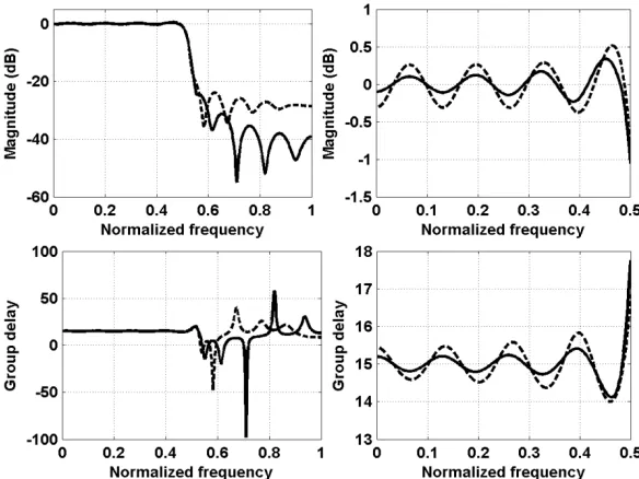
Fig. 3.1 Magnitude and group delay responses of IIR filters designed in Example 1. Solid curves: designed by the proposed method. Dashed curves: designed by the least 4-power method [7]. ...33

Fig. 3.2 Magnitude and group delay responses of IIR filters designed in Example 1 with peak error constraints. Solid curves: designed by the proposed method. Dashed curves: designed by the WLS method [11]. ...35

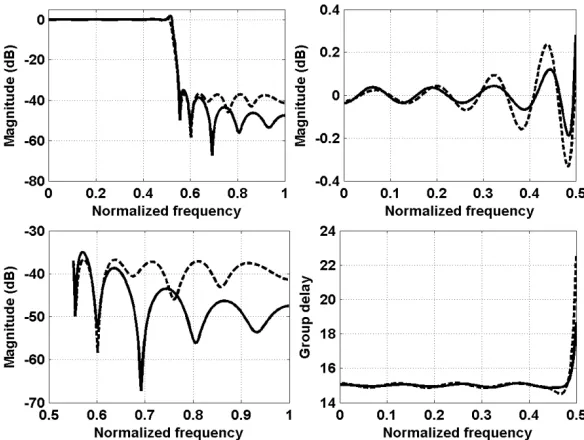
Fig. 3.3 Magnitude and group delay responses of IIR filters designed in Example 2. Solid curves: designed by the proposed method. Dashed curves: designed by the WISE method [28]. ...37

Fig. 3.4 Variation of maximum pole radii of designed IIR digital filters with respect to the regularization parameter α. ...38

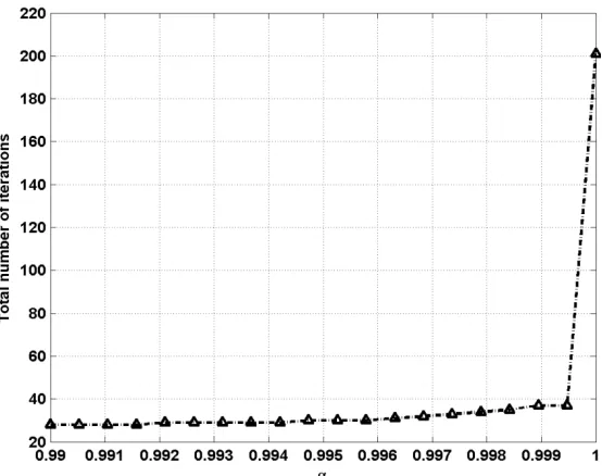
Fig. 3.5 Variation of total number of iterations with respect to the regularization parameter α. ...39

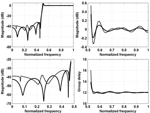
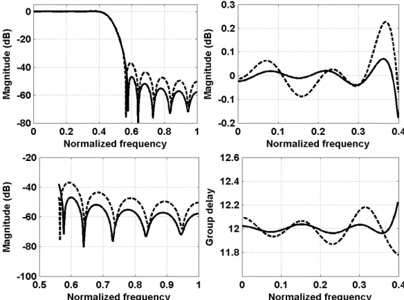
Fig. 3.6 Magnitude and group delay responses of IIR filters designed in Example 3. Solid curves: designed by the proposed method. Dashed curves: designed by the WLS method with linearized argument principle based stability constraint of [21]. ...40

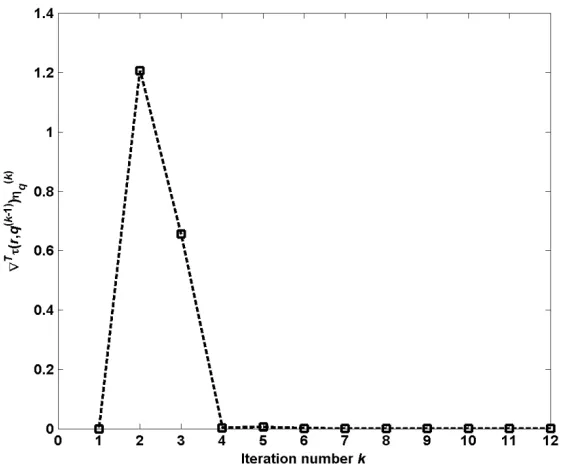
Fig. 3.7 Values of , during the design procedure of the proposed

method...41

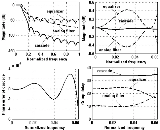
Fig. 3.8 Magnitude and group delay responses, and phase error of IIR filter designed in Example 4. Solid curves: cascaded system. Dashed curves: equalizer designed by the proposed method. Dash-dotted curves: analog filter. ...43

(16)

Fig. 4.2 Magnitude of weighted complex error of IIR filters designed in Example 1. Solid curves: designed by the proposed method. Dashed curves: designed by the SOCP method

[19] ...61

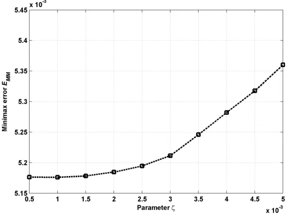
Fig. 4.3 Variation of minimax error versus parameter . ...62

Fig. 4.4 Magnitude and group delay responses of IIR filters designed in Example 2. Solid curves: designed by the proposed method. Dashed curves: designed by the SM method [8]. ...64

Fig. 4.5 Magnitude of weighted complex error of IIR filters designed in Example 2. Solid curves: designed by the proposed method. Dashed curves: designed by the SM method [8]. ...64

Fig. 4.6 Variation of discrepancy between and versus iteration number . ...65

Fig. 4.7 Magnitude and group delay responses of IIR filter designed in Example 3. ...67

Fig. 4.8 Magnitude of weighted complex error of IIR filter designed in Example 3. ...67

Fig. 4.9 Design characteristics and errors of IIR differentiator designed in Example 4. ...69

Fig. 4.10 Magnitude of weighted complex error of IIR differentiator designed in Example 4...70

Fig. 5.1 Flowchart of the complete design method. ...85

Fig. 5.2 Magnitude and group delay responses of IIR filters designed in Example 1. Solid curves: designed by the proposed method. Dashed curves: designed by the SM method [8]. ...90

Fig. 5.3 Magnitude of complex approximation error | | in Example 1. Solid curves: designed by the proposed method; Dashed curves: designed by the SM method [8]. ...90

(17)

Fig. 5.5 Magnitude of complex approximation error | | in Example 2. Solid curves: designed by the proposed method; Dashed curves: designed by the Remez multiple exchange method [25]. ...93

Fig. 5.6 Design characteristics and errors of the differentiator of order 8 in Example 3. Solid curves: designed by the proposed method. Dashed curves: designed by the modified EW method [18]. ...95

Fig. 5.7 Design characteristics and errors of IIR differentiator of order 5 designed in Example 3. Solid curves: designed by the proposed method. Dashed curves: designed by the modified EW method [18]. ...96

Fig. 5.8 Magnitudes of complex approximation error | | of IIR differentiators designed in Example 3. Solid curves: differentiator of order 8; Dashed curves: differentiator of order 5. ...96

Fig. 5.9 Magnitude and group delay responses of IIR filters designed in Example 4. Solid curves: designed by the proposed method (ρmax = 1) followed by rescaling q through

(5.32) and solving (4.27). Dash-dotted curves: designed by the proposed method (ρmax =

0.98). Dash curves: designed by the SM method [8]. ...98

Fig. 5.10 Magnitude of complex approximation error | | in Example 4. Solid curves: designed by the proposed method (ρmax = 1) followed by rescaling q through (5.32) and

solving (4.27). Dash-dotted curves: designed by the proposed method (ρmax = 0.98). Dash

(18)

L

IST OF

A

BBREVIATIONS

BIBO Bounded Input and Bounded Output

DSP Digital Signal Processing

FIR Finite-duration Impulse Response

IDFT Inverse Discrete Fourier Transform

IIR Infinite-duration Impulse Response

LMI Linear Matrix Inequality

LP Linear Programming

PSD Positive Semi-Definite

QP Quadratic Programming

SDP Semi-Definite Programming

SOC Second-Order Cone

SOCP Second-Order Cone Programming

WISE Weighted Integral of the Squared Error

(19)

C

HAPTER

I

NTRODUCTION

A digital filter is a computational tool to extract useful information and remove undesired components from input sequences, and simultaneously generate output sequences. Digital filters can be implemented on general-purpose computers or some specific hardware. Some advantages of digital filters over analog filters are listed below:

1. Digital filters are programmable, which means that the characteristics of digital filters can be easily modified leaving the hardware unchanged.

2. Digital filters can be conveniently designed, tested and implemented on general-purpose computers.

3. Compared with analog filters, the characteristics of digital filters are much more consistent with respect to time and temperature.

4. Digital filters are very versatile in their ability to process signals in a variety of ways, which includes the ability of some types of digital filters to adapt to the changes of input signals.

As one of important and fundamental areas in digital signal processing (DSP), the research work on digital filter designs started in the 1960s. Although many design methods have been proposed so far, nowadays the research on digital filter designs is still active. More efficient and robust design techniques are being proposed with the advances of DSP and mathematical theories. On the other hand, the emergence of new classes of digital filters also stimulates the development of digital filter designs.

(20)

The characteristics of a digital filter can be described by its transfer function. The transfer function of an FIR digital filter is a polynomial function of , i.e.,

(1.1)

where

… (1.2)

1 … (1.3)

Here, the superscript represents the transpose of a vector or matrix. For an IIR digital filter, its transfer function is a rational function of , i.e.,

∑

1 ∑ (1.4)

where

… _(1.5)

1 … (1.6)

The frequency responses of digital filters are calculated by evaluating their transfer

functions on the unit circle, that is, = | and = | .

From (1.1), it can be found that all poles of an FIR digital filter are located on the origin of the plane. However, all poles of an IIR digital filter must be constrained inside the unit circle of the plane for stability.

In this dissertation, we mainly study IIR filter design problems. Generally speaking, an IIR filter design problem can be stated as follows:

(21)

whose frequency response can best approximate the given ideal frequency response under some design criterion.

In the proposed design methods, we assume that all the numerator and denominator coefficients are real values. Nevertheless, all the design methods presented in this dissertation can be readily extended to IIR filter designs with complex coefficients. It is noteworthy that besides the models in the direct form of (1.1) and (1.4), there are some other useful models, such as zero-pole, lattice, and state-space. However, in this dissertation, we only consider the direct form due to its simplicity in formulating design problems.

Because of the close relationship between FIR and IIR digital filters, in this chapter we shall first introduce FIR digital filter designs. Then, the history of IIR digital filter designs will be briefly reviewed. Motivations and objectives of the research work reported in this dissertation will be described later. The organization of the rest of the dissertation and main contributions will be finally presented in this chapter.

1.1 Introduction to FIR Digital Filter Design

Compared with IIR digital filters, FIR digital filters have several advantages:

1. Since all poles of an FIR digital filter are fixed at the origin of the plane, the frequency response of an FIR digital filter is determined by its zeroes. Thereby, no stability concern exists for FIR digital filter designs.

2. By utilizing (anti-)symmetric structures, FIR digital filters with exactly linear phase over the whole frequency band can be easily achieved. However, except for some special cases, it is difficult to design an IIR digital filter, which has exactly linear phase over the whole frequency band.

(22)

convex optimization problem. Hence, globally optimal solutions cannot be definitely attained.

From the 1960s, a large part of efforts have been devoted to develop efficient approaches to design phase FIR digital filters [1]-[2]. As mentioned above, linear-phase FIR digital filter coefficients demonstrate (anti-)symmetric structures. Thus, the number of free variables of design problems can be reduced by about one half. Furthermore, besides a constant-delay component, the frequency response of a linear-phase FIR digital filter can be expressed by a trigonometric function of filter coefficients.

The first well-known design technique is the Fourier series method [1]-[2], in which a desired frequency response is first expanded as its Fourier series and then truncated to a finite length. This method suffers from Gibbs’ oscillations due to the discontinuity of the desired frequency responses. In order to reduce Gibbs’ oscillations near the cutoff frequencies, a smooth time-limited window, such as the Hamming window and the Kaiser window, is multiplied with the coefficients of the Fourier series. This method has two obvious drawbacks: First of all, FIR digital filters designed by this window method are not optimal in any optimization sense. Moreover, the frequency band edges of the designed FIR filters cannot be the same as specified.

The second design technique is called the frequency sampling method [1]-[2]. The desired frequency response is specified on a set of discrete frequency points, and then the inverse discrete Fourier transform (IDFT) is used to obtain the discrete-time impulse response. Despite its easy implementation, the performance of this method is not good enough compared with the design methods using optimization techniques.

(23)

designing linear-phase FIR digital filters in the minimax sense. Some other linear constraints can be further incorporated in this LP design method.

In order to achieve the linear phase over the whole frequency band, linear-phase FIR filter coefficients should be (anti-)symmetric, and the group delay can only be set equal to /2, where denotes the filter order. If one wants to achieve a lower group delay, the filter length has to be correspondingly reduced. However, sometimes this is impracticable because of the strict design specifications. On the other hand, FIR digital filters with nonlinear phase responses are useful in many applications. Therefore, we are also interested in general FIR digital filter designs, where the ideal frequency responses can be arbitrarily selected.

It can be observed that the transfer function in (1.1) is a linear function of filter coefficients . In general, an FIR filter design problem can be expressed as an equivalent convex optimization problem [5]. The techniques of transforming an FIR design problem into an equivalent convex optimization problem are very useful in the latter discussion of IIR digital filter designs. Let represent the desired frequency response to be approximated. In the WLS sense, the approximation error can be defined by

Ω

2 constant

(1.7)

where ≥ 0 denotes a given weighting function, and Ω is the union of frequency bands of interest. In (1.7), the matrix and vector are defined as follows

· Re

Ω (1.8)

· Re

Ω (1.9)

(24)

positive definite, the WLS approximation error is a convex quadratic function of . If no other constraints need to be incorporated in the WLS design problem, the optimal filter coefficients can be readily obtained by solving the linear equation = .

Some numerical methods, e.g., Newton’s method, can be utilized here to find . If

only linear constraints are incorporated, the design problem can be formulated as a quadratic programming (QP) problem. The approximation error can also be expressed by

/ / _constant _(1.10)

where / _{denotes the square root of , and} _{represents the Euclidean norm of a}

vector . By introducing an auxiliary variable , the WLS design problem can be equivalently expressed by

min (1.11)

s.t. / / (1.11.a)

It is known that (1.11.a) is a second-order cone (SOC) constraint, and the above design problem is essentially an SOCP optimization problem. Some other linear or (convex) quadratic constraints can be further incorporated in (1.11).

In the minimax sense, the FIR filter design problem is defined by

min max

Ω | | (1.12)

where the (weighted) complex approximation error is defined by

, Ω (1.13)

(25)

| | over Ω , the original minimax design problem (1.12) can be equivalently written by

min (1.14)

s.t. | | , Ω (1.14.a)

By reformulating | |, the constraint (1.14.a) can be transformed to the following SOC constraint

(1.15)

where

Re

Im (1.16)

Re

Im (1.17)

In (1.16) and (1.17), Im · represents the imaginary part of a complex value. For simplicity, the constraint (1.15) can be enforced on a set of discrete frequency points densely sampled over Ω . Obviously, using the SOC constraint (1.15), the minimax design problem (1.14) can be converted to an SOCP problem.

As a generalization of the WLS and minimax criteria, the -norm error criterion is

(26)

1.2 Introduction to IIR Digital Filter Design

Compared with FIR digital filters, IIR digital filters can achieve much better performance under the same set of design specifications. However, IIR filter designs face more challenges due to the presence of the denominator in (1.4). The major difficulties we encounter are as follows:

1. Since the poles of an IIR digital filter can be anywhere in the plane, in general, IIR filter design problems are nonconvex optimization problems. Accordingly, there exist many local optima on error performance surfaces, and globally optimal solutions cannot be definitely achieved or even verified.

2. If phase (or group delay) responses are also of concern, stability constraints must be incorporated in design procedures. However, when the denominator order is larger than 2, the stability domain cannot be expressed as a convex set with respect to denominator coefficients .

The techniques of invariant impulse response, matched- transformation, and bilinear transformation are widely used to achieve an IIR digital filter from a given analog filter [1]-[2]. These design techniques are straightforward, and can naturally guarantee the stability of obtained IIR digital filters. However, these techniques can only be applied to transform standard analog filters, such as lowpass, highpass, bandpass and bandstop filters, into digital counterparts.

(27)

If phase (or group delay) responses are also under consideration, IIR filter design problems become more complicated. As in FIR filter design problems, the WLS and minimax criteria are also widely used in practical IIR filter designs. Like (1.7), the WLS approximation error of an IIR filter design can be defined by

Ω

(1.18)

where

(1.19)

As in (1.7) and (1.13), and represent the given weighting function and the desired frequency response, respectively. Similarly, the minimax approximation error is expressed by

max

Ω | | (1.20)

where the (weighted) complex approximation error is given by

(1.21)

The objective of our design problems is to minimize these approximation errors subject to some other constraints. It is worth noting that although the complex approximation error is differentiable over Ω , the minimax approximation error is a nondifferentiable function of . Therefore, it is inconvenient to directly manipulate

in practical designs. Besides the WLS and minimax criteria, some other design criteria, such as the Lp-norm error criterion, where the approximation error is defined by

(28)

In general, IIR filter design methods can be classified into two groups: direct and indirect ways. It should be mentioned here that direct design methods are often referred to as those methods that are carried out directly in the domain and indirect design methods are generally considered to be those methods based on analog filters [2]. In this dissertation, however, we adopt somewhat different definitions for direct and indirect design methods. In the direct design strategy, the best approximation to a given ideal frequency response is found without any intermediate step. In the indirect design strategy, a design problem is first transformed to an FIR filter design problem. Then, model reduction techniques can be deployed to achieve an IIR digital filter, which can best approximate the FIR digital filter. As presented before, in general, FIR filter design problems can be equivalently cast as convex optimization problems and then efficiently solved. Therefore, the performances of indirect design methods are mainly determined by the second step, i.e., FIR approximation by IIR digital filters. In this dissertation, we mainly study IIR filter designs using the direct design strategy. But it should be mentioned that the proposed design methods can be straightforwardly applied in indirect IIR filter designs by replacing the desired frequency response by a well-defined

FIR frequency response and the frequency bands of interest Ω by the whole frequency band [0, ].

(29)

time-domain stability constraints try to control the l2-norm of denominator coefficients at a

reasonable level or force the impulse responses of the inverse filter = 1/ to approach 0 as ∞. The frequency-domain stability constraints are mainly derived from complex analysis. Compared with time-domain stability constraints, frequency-domain stability constraints are much more tractable. Many frequency-frequency-domain stability constraints are formulated in convex forms, such that they can be readily incorporated in optimization-based design methods. However, these convex frequency-domain stability constraints are only sufficient conditions for stability. This means that some stable IIR filters could be excluded from the set of admissible solutions. For the implicit description, the stability of designed IIR filters can be automatically guaranteed by design procedures. For example, by adjusting the step size at each iteration to keep all the updated poles staying inside the stability domain, some sequential design methods can always obtain stable designs without any explicit stability constraint.

1.3 Motivations and Objectives

(30)

developed for convex optimization. Actually, many well-developed mathematical tools are available for solving these convex optimization problems.

So far, a large number of IIR filter design methods have been proposed. Although the effectiveness of these methods has been demonstrated by many examples in the literature, their design performances could be impaired by insufficient stability constraints adopted by these design methods, or their practical applications could be restricted by the unguaranteed convergence of these design methods. These issues will also be addressed in this dissertation.

Although it is difficult to completely resolve the nonconvexity and stability issues of IIR filter design problems, in this dissertation we shall try to alleviate these difficulties to some extent, such that the proposed design methods have more chances to approach optimal designs than traditional design methods.

1.4 Organization of the Dissertation

(31)

1.5 Main

Contributions

In this dissertation, we are mainly studying IIR filter design problems under the WLS and minimax criteria. All the proposed design methods are primarily devoted to tackle the nonconvexity and stability issues of design problems. The main contributions of the research work reported in this dissertation are summarized as follows:

Firstly, a novel stability condition is derived from the argument principle of complex analysis. Compared with some other frequency-domain stability conditions, it is both sufficient and necessary. In practice, however, this stability condition is still nonconvex. Thereby, some approximation techniques need to be employed to achieve an approximate stability condition in a quadratic form, such that it can be readily combined with the sequential WLS design procedure. This approximate stability condition can guarantee the stability of designed IIR digital filters, if the sequential design method is convergent and a regularization parameter is appropriately selected.

Secondly, convex relaxation techniques are introduced in minimax IIR filter designs. The major idea of this design strategy is to relax the original nonconvex design problems so as to achieve design problems in convex forms, which can be efficiently and reliably solved. Furthermore, by solving these relaxed design problems, we can obtain some important information about optimal solutions of the original nonconvex design problems, e.g., lower and upper bounds of the minimum approximation error. In this dissertation, two different types of convex relaxation techniques are used in minimax designs. The resulting relaxed design problems are formulated, respectively, as SOCP and SDP optimization problems. In the SDP formulation, a sufficient condition for an optimal design of the original design problem is presented, which can be used to detect the optimality of IIR filters designed by the proposed design method.

(32)

(33)

C

HAPTER

II

R

EVIEW OF

IIR

D

IGITAL

F

ILTER

D

ESIGN

M

ETHODS

Compared with an FIR filter design problem, an IIR filter design problem is more challenging due to its nonconvex nature. As mentioned before, the nonconvexity is mainly incurred by the denominator whose roots can be anywhere in the plane. Recently, a number of design methods [7]-[43] have been proposed to solve various IIR filter design problems. These methods can be roughly classified into three groups: sequential design methods [7]-[27], nonsequential design methods [28]-[32], and model reduction methods [33]-[43]. We shall briefly review some important design methods in this chapter. It is worth emphasizing that this classification is not unique, since strictly some methods can be classified into two groups. For example, some model reduction methods also involve sequential procedures. We group these methods based on their basic design strategies. Another point, which should be mentioned here, is that many design methods depend on a variety of optimization methods [44]-[48] (e.g., quasi-Newton methods, sequential quadratic programming method, simplex method, and interior-point methods) to solve these design problems. Essentially speaking, these optimization methods involve iterations. Nevertheless, in this dissertation, we shall focus on convex formulations and analyses of IIR filter design problems. Thereby, these optimization methods can be viewed as black-box subroutines, which can be invoked to solve practical problems formulated by designers. These optimization methods have been provided by many well-developed software.

2.1 Sequential

Design

Methods

(34)

The Steiglitz-McBride (SM) scheme [49] is adopted in many sequential design methods [7]-[13] under various design criteria. At each iteration, the denominator of an approximation error is replaced by its counterpart obtained at the previous iteration and combined with a prescribed weighting function. Then, the original objective functions can be approximated by convex functions of filter coefficients. Accordingly, the IIR filter design problems can be transformed to convex optimization problems. Different stability constraints are utilized in these design methods, such as the positive realness [7]-[8], [10]-[11], the Lyapunov theory [12], and the argument principle [13] based stability constraints. Although the SM scheme does not completely tackle the nonconvexity of IIR filter design problems, compared with classical descent techniques, it can avoid being stuck at local minima near the initial points. Its effectiveness has been demonstrated by many examples reported in the literature. The major drawback of the SM design approaches is that the convergence of these sequential methods cannot be definitely guaranteed.

A design strategy similar to the SM scheme is used by the design method proposed

in [14]. By introducing an inverse filter corresponding to the denominator ,

i.e., = 1, numerator and denominator designs can be decoupled into two separate optimization problems. The optimal numerators can be explicitly expressed in terms of coefficients of the inverse filter. The denominator design can be simplified as a QP problem by adopting an approximation technique similar to the SM scheme. The stability of designed filters can be ensured by flipping the poles outside the unit circle into the inside at each iteration. A variant of the design method [14] has been presented in the time domain by [15]. Instead of the approximation error defined by (1.18), the design objective is to minimize the model-fitting error between the desired impulse responses and significant samples of an IIR digital filter system, i.e., where = [ 0 1 … ]T_{denotes the impulse responses of} _and _{= [} ₀ ₁ _…

]T represents the desired impulse responses.

(35)

the complex approximation error of the IIR filter obtained at the previous iteration. Then, by solving a WLS design problem constructed by the new weighting function, the minimax error can be simultaneously reduced. The major drawback of this design method is that stability constraints cannot be directly incorporated into the design procedure. Thus, the resulting filters may be unstable. A similar strategy is also used by the minimax design method proposed in [17]. However, the magnitude of the complex approximation error of the IIR filter obtained at the previous iteration is directly employed to determine the weighting function.

Since the frequency response is a nonlinear function of denominator coefficients, many design methods use its Taylor series to simplify design problems. Based on this idea, a minimax design method has been developed by [18]. At each iteration, given a denominator the optimal numerator design is first obtained. By fixing the numerator, is then approximated by its first-order Taylor series with respect

to denominator coefficients, i.e., +∆ ,

where denotes the iteration index and ∆ represents a descent direction of denominator coefficients to be determined. Using this linearized frequency response, the design problem at each iteration can be formulated as a convex optimization problem. Line search is employed to guarantee the convergence of this sequential design method. Provided the initial design is stable, the stability of a designed IIR filter can be guaranteed by adjusting the step size at each iteration, such that the updated

denominator coefficients = + ∆ is always within the stability domain. Generally, the computational complexity of this design method is relatively low. However, since the descent direction is determined based on the local information, the design performance is sensitive to the selection of initial points.

(36)

a first-order section if the denominator order is odd. Then, the resulting stability constraints can be expressed by a set of linear inequality constraints in terms of these factorized denominator coefficients. The advantage of using the factorized denominator is that the corresponding stability constraints can be easily expressed by a set of linear inequality constraints, which are sufficient and almost necessary for stability. Different from the SOCP method [19], the GN design method [20] adopts numerator and denominator polynomials both in the direct form. The Rouché’s theorem based stability constraint is used in the GN design method, which is less restrictive than the positive realness based stability constraint [32]. Both the SOCP and GN design methods suffer the same drawback as SM design methods regarding nonguaranteed convergence. Another design method using a similar design strategy has been proposed by [21]. A linearized argument principle based stability constraint is employed to guarantee the stability of designed IIR filters.

By adopting linearized frequency responses, the approximation errors in [19]-[21]

can generally be written as convex quadratic forms, i.e., ∆ ∆ ∆ , where ∆

denotes a descent direction of filter coefficients , represents the gradient of the original approximation errors with respect to , and is a positive definite matrix generally determined by the gradient. The matrix can be viewed as an estimate of the Hessian of the original approximation errors. The real Hessian of the approximation error is utilized by the design method proposed in [22] under the Lp-norm error criterion. The

modified Newton’s method is employed to solve the design problem. The stability of designed IIR filters can be ensured by a similar strategy adopted in [18].

(37)

the multistage design method [23], a minimax design [24] can be obtained by successively optimizing numerators using the reweighting technique proposed by [16].

A special class of sequential design methods have been developed by [25]-[26] based on a sufficient condition for the optimal rational approximation, which states that the approximation error has a specific number of extremal points over the frequency bands of interest. The Remez exchange algorithm is employed to identify these extremal points. In order to achieve satisfactory designs, the initial point should be selected close enough to the optimal solution to guarantee the convergence of the sequential procedure. The Remez exchange algorithm is also employed by the minimax design method proposed by [27]. However, the transfer function of an IIR filter in [27] is in the form of a parallel connection of two allpass filters.

2.2 Nonsequential Design Methods

In practice, optimal designs cannot be definitely achieved even using the sequential design methods described earlier. In practice, if an obtained solution satisfies the prescribed specifications, it can be taken as a successful design. On the other hand, as mentioned before, the convergence of some sequential design methods cannot be always ensured. Therefore, some design methods [28]-[30] abandon the sequential design strategy and try to strictly formulate design problems as unconstrained optimization problems, which are then solved by a variety of efficient and robust unconstrained optimization methods. In [28]-[29], the objective functions of the WLS design problems consist of two components. The first part reflects the WLS approximation error, while the second one serves as a barrier function to control poles’ positions for stability. Gradient-based optimization methods can be applied to solve these unconstrained optimization problems. In general, designers should provide at least the gradients of the objective functions. Satisfactory designs can be obtained by repeating the design procedures from different initial points.

(38)

is decomposed as a cascade of second-order sections. The Fletcher-Powell algorithm [50] is employed in [30] to solve this nonlinear design problem. The stability of designed filters can be ensured by the same technique used in [18].

In [31], the design problem is first formulated as a multiple-criterion optimization problem, in which both magnitude and group delay approximation errors are simultaneously minimized. This multiple-criterion design problem can be further transformed to a constrained nonlinear programming problem and then solved by sequential quadratic programming method. In [30] and [31], the design problems are both formulated under the Lp-norm error criterion.

An LP design method has been proposed by [32] under the minimax criterion. In order to simplify the design problem, the denominator of the complex approximation error defined by (1.21) is neglected, such that the peak error constraint | |≤ is transformed to a quadratic form, which can be further approximated by a set of linear inequality constraints. The stability of designed IIR digital filters can be assured by a positive realness based constraint. Despite its simplicity, it is hard to obtain a true minimax design by this method. However, in practice, we can use this method at the beginning of some sequential design methods to achieve initial designs [18].

2.3 Model Reduction Design Methods

Sequential and nonsequential design methods described above both belong to the category of direct design methods, that is, given a desired frequency response, we can directly obtain an IIR digital filter using these design methods. Another category of methods [33]-[43] design IIR digital filters through an indirect way. An FIR digital filter satisfying prescribed specifications are designed first, and then model reduction techniques are applied to approximate the FIR digital filter by a reduced-order IIR digital filter. Specifically, for the WLS and minimax designs, the desired frequency response

in (1.18) and (1.21) is replaced by the frequency response of an FIR digital

(39)

The indirect design scheme has two advantages:

1. Since an FIR filter design problem can be conveniently formulated as a convex optimization problem in a finite-dimensional space, which has been extensively studied, the second step becomes the kernel of an IIR filter design problem. By contrast with direct IIR digital filter design methods, the FIR approximation by IIR digital filters is less complicated.

2. In most of indirect design methods, the FIR approximation by IIR digital filters can substantially guarantee the stability of designed IIR digital filters, which also facilitates the design procedures.

However, even though the optimal results can be obtained in each step of indirect design methods, it cannot be concluded that the optimal solutions of the original IIR filter design problems can be definitely attained by indirect design methods.

2.4 Filter Designs Using Convex Optimization

The mathematics of convex optimization [51]-[55] has been studied for about one century. However, new research interests in this topic have been rejuvenated due to the advances of interior-point methods developed in the 1980s. Recently, many applications of convex optimization have been discovered in various fields of applied science and engineering, such as automatic control system, signal processing, VLSI circuit design, mechanical structure design, statistics and probability, and finance. There are many advantages of utilizing convex optimization to solve practical engineering problems. The most important one is that when a problem is equivalently cast as a convex optimization problem, any local solution is also a global optimum. Furthermore, a convex optimization problem can be solved very efficiently and reliably, using interior-point methods [70]-[71].

(40)

problems. Thus, the optimal designs can be definitely obtained. Compared with FIR filter designs, allpass filter designs face more challenges due to the same difficulties as encountered in IIR filter designs. An important property which can be exploited is the mirror symmetric relation between numerator and denominator, i.e., = . Note that if the transfer function of an allpass filter is still defined by (1.4) with = , this property can be described by a set of linear equality constraints = for = 0, 1, …, . Therefore, most of optimization-based IIR filter design methods described in the proceeding sections can also be used to design allpass filters. However, this design strategy does not make full use of the characteristics of allpass digital filters, and hence some computation resources will be wasted. Since allpass filters have the fullband unity magnitude responses, the design problems can also be formulated in terms of phase response approximation error. Let and denote, respectively, the ideal phase

response to be approximated and the phase response of the denominator . Then, the phase response approximation error can be calculated by =

2 . Since the tangent function is an increasing function within [ /2, /2], we can reduce the phase response approximation error by minimizing the error limit of

tan over Ω , where tan = _∑∑ and = . It

can be seen that the approximation error is a linear fractional function of denominator coefficients. Accordingly, allpass filter design problems can be transformed into quasi-convex optimization problems.

(41)

C

HAPTER

III

IIR

D

IGITAL

F

ILTER

D

ESIGN WITH

N

EW

S

TABILITY

C

ONSTRAINT

B

ASED ON

A

RGUMENT

P

RINCIPLE

Stability is a critical concern in an IIR filter design problem. So far, many stability constraints have been proposed in frequency domain. However, some of these stability constraints are only sufficient conditions, which means stable filters could be excluded from the feasible sets of design problems. Recently, a stability constraint based on the argument principle of complex analysis has been developed in [21], which is both sufficient and necessary. By truncating the higher-order Taylor series components, the resulting stability constraint becomes a linear equality constraint. However, through a large number of simulations, it is found that this linearized constraint could be invalid in some situations. As an attempt to resolve this problem, a new stability constraint is proposed in this chapter, which is also based on the argument principle. Unlike the linearized stability constraint in [21], this new stability constraint is approximated in a quadratic form. The effectiveness of this approximate stability constraint can be demonstrated by theoretical analysis and many simulation examples.

This chapter is organized as follows. In Section 3.1, a sequential SOCP method without any stability constraint is first introduced to design IIR digital filters in the WLS sense. Then, peak error constraints are incorporated as SOC constraints. In Section 3.2, a novel stability constraint is developed from the argument principle of complex analysis, which is then combined with the sequential design method. Design examples are presented in Section 3.3 to illustrate the performance of the proposed method.

3.1 WLS Design of IIR Digital Filters

3.1.1 Sequential Design Procedure

(42)

min _(3.1)

where the approximation error has been defined by (1.18). By introducing an auxiliary variable , (3.1) can be reformulated as

min (3.2)

s.t.

Ω

(3.2.a)

Because of the existence of denominator in the integrand, the constraint (3.2.a) cannot be cast as a convex form. Here, we employ the Steiglitz-McBride scheme [49] to simplify the above design problem. This strategy has been widely used by many design methods [7]-[13]. At the th iteration, the constraint (3.2.a) is modified as

Ω

(3.3)

where denotes the current filter coefficients to be determined, and the vector is defined by

(3.4)

The major modification is on the weighting function, i.e., , which is defined by

(43)

Here, the denominator obtained at the previous iteration is taken into (3.5) to construct a new weighting function. Obviously, the left hand side of the inequality (3.3) is in a convex quadratic form with respect to , which can be expressed by

(3.6)

where

· Re

Ω (3.7)

Since is a symmetric and positive definite matrix, (3.6) can be further cast into an SOC constraint

/

(3.8)

where / _{denotes the square root of the matrix .}

In practice, for the sake of robustness of the sequential design procedure, the filter coefficients are updated by

, 0 1 (3.9)

where is the coefficient vector obtained at the previous iteration, is a fixed step

size, and is the updating vector at the current iteration. By specifying = 1 or

equivalently = 0 for all ≥ 0, the design problem (3.2) with the SOC constraint (3.8) can be rewritten by

min (3.10)

s.t. 0 (3.10.a)

(3.10.b)

(44)

/

(3.11)

/

(3.12)

The sequential design procedure continues until the following condition is satisfied

(3.13)

where is a prescribed convergence tolerance, or exceeds a specified maximum number of iterations. Although so far the convergence of the sequential procedure has not been definitely guaranteed, the effectiveness of the SM scheme has been demonstrated by many filter examples in a variety of papers.

3.1.2 Peak Error Constraint

In [7] and [8], linearized peak error constraints have been developed to control the peak errors. Here, we shall reformulate the peak error constraints as a set of SOC constraints, which can better approximate the true peak error constraints.

The peak error constraints can be strictly expressed by

, Ω , 1,2, … , (3.14)

where denotes the prescribed peak error limit at a specific frequency . Like the difficulty encountered in formulating the design problem (3.2), the real peak error constraint also has the denominator on the left hand side of (3.14). Adopting a similar technique employed in (3.3) and rearranging terms, we obtain

· , Ω , 1,2, … ,

(3.15)

(45)

Re / _(3.16)

Note that in [7] and [8] the IIR filter design problems are cast, respectively, into LP and QP problems, in which only linear constraints can be handled. Therefore, the approximation of a circle by a regular polygon is applied to linearize the constraint (3.14). Although this approximation is applicable when the edge number of a regular polygon is large enough, the total number of peak error constraints is rapidly increased.

3.2 Argument

Principle

Based Stability Constraint

A new stability constraint based on the argument principle is to be developed in this section. First of all, the argument principle is to be reviewed. The stability constraint derived from the argument principle is then to be approximated by a quadratic constraint and combined with the sequential design method described in Section 3.1.

3.2.1 Argument Principle

If is analytic in a region enclosed by a contour in the plane except at a finite number of poles, let be the number of zeros and be the number of poles of

the function in , where each zero and pole is counted according to its multiplicity. Then we have

1

2 (3.17)

This result is called the argument principle [64]-[65].

In order to develop a practical stability constraint for IIR digital filter designs, we consider the following monic polynomial function

(46)

Obviously, has zeros and no poles in the finite plane. The contour is chosen as an origin-centered circle with a prescribed maximum pole radius , i.e., : | |

, 1 . Then, according to the argument principle described above, all zeros of lie strictly in the region enclosed by , if and only if the following equality condition is satisfied

1

2 (3.19)

The integral in (3.19) is carried out counterclockwise along . Note that

ln

ln| | arg

(3.20)

where arg denotes the argument of . The first term on the right-hand side of the second equation of (3.20) is always equal to zero, since the logarithmic function is single-valued and is closed. According to (3.18), arg can be expanded as arg

on , and then the stability constraint (3.19) can be simplified as

1

2 arg 0 (3.21)

Thus, the stability constraint (3.21) of an IIR digital filter is stated as: An IIR digital filter with the denominator is stable, if and only if the total change in the argument of

is equal to 0, when the integral is carried out along counterclockwise.

3.2.2 Argument Principle Based Stability Constraint

The polynomial function can be expressed as

| (3.22)

(47)

Re Re (3.23)

Im Im (3.24)

The argument of is then computed by

arg arctan

arctanIm Re

(3.25)

By taking differentials with respect to on both sides of (3.25) and rearranging terms, we have

arg

| | (3.26)

where

diag 0,1, … , (3.27)

Re

1 cos cos

cos cos 1

(3.28)

In (3.27), diag , , … , represents a diagonal matrix with on its th diagonal. By taking (3.26) into (3.21) and computing the integral over [0, ], the stability constraint (3.21) is transformed to

, , 0 (3.29)

(48)

,

2| | (3.30)

If has (≤ ) roots outside and – roots inside , it can be verified that

, = . Then, given a denominator , , has a stair shape with respect to .

Unfortunately, the stability constraint (3.29) cannot be directly incorporated into the design problem (3.10), due to the following difficulties:

1. The stability condition (3.29) represents a nonlinear equality constraint.

2. The matrix , is dependent on denominator coefficients .

3. The matrix , is indefinite.

The first difficulty can be overcome by adopting the following inequality

, , (3.31)

Decreasing makes more poles move inside the circle . When 0 < < , all poles will lie inside . In order to tackle the second difficulty, we adopt a similar technique used in Section 3.1. At the th iteration, , is modified by

, , (3.32)

Since , is an indefinite matrix, this explicit stability constraint cannot be

directly transformed into an SOC constraint. Therefore, we combine the stability constraint with the constraint (3.6) and obtain

(3.33)

where

1 , (3.34)

(49)

In (3.35), denotes a zero matrix of size -by- . Accordingly, in (3.11) and

(3.12) is replaced by . If the sequential design procedure described in Section 3.1

converges, it follows that = → 1 for [0, ] as → +∞. Then,

we can obtain that

,

2| | ·

,

(3.36)

In practice, we can decrease to achieve lower , , which corresponds to

decreasing of (3.31) as +∞. Therefore, besides the prescribed maximum pole radius , the regularization coefficient also plays an important role of restricting poles’

locations. It is noteworthy that decreasing makes approach an indefinite matrix, which cannot be used to formulate the SOC constraint in (3.10). Thus, cannot be too small. Fortunately, generally is large enough to guarantee the positive definiteness of

. Simulation experience indicates that is normally within the range [0.99, 0.999999]. The effects of on the final design results will be illustrated by Example 2 in the next section.

Finally, the major steps of the proposed sequential design method are summarized below:

Step 1. Given an ideal frequency response , filter orders and , a weighting

function , set = 0 and choose an initial guess .

Step 2. Set = +1, and compute by (3.5), by (3.34) and by

(3.16). Then utilize to calculate by (3.11) and by (3.12).

Finally, solve for the SOCP problem (3.10) with peak error constraints (3.15).

(50)

or exceeds a predetermined maximum number of iterations, terminate the sequential design procedure. Otherwise, go to Step 2 and continue.

3.3 Simulations

In this section, four examples are presented to demonstrate the effectiveness of the proposed design method. At each iteration, the SOCP problem (3.10) is to be solved by SeDuMi [66] in MATLAB environment. Besides the peak and errors of magnitude (MAG) and group delay (GD), we also adopt the WLS approximation error defined by (1.18) to evaluate design performances. In our designs, the step size in (3.9), the convergence tolerance in (3.13), and the maximum number of iterations are always chosen as 0.8, 10-6, and 200, respectively.

3.3.1 Example 1

The first example taken from [7] is to design a lowpass digital filter. The ideal frequency response is defined by

0 0.5

. . _0.5

(51)

It can be seen that the proposed method can achieve much better performances in the WLS sense.

Table 3.1 Filter Coefficients ( to and to ) of IIR digital filters Designed in Example 1

Proposed WLS design

~ -1.0713e-002 -1.3178e-002 8.9219e-003 9.5276e-004 -8.1651e-003

~ -1.9799e-003 1.0818e-002 1.7638e-003 -1.5605e-002 -8.9659e-004

~ 2.5278e-002 -1.2083e-003 -5.2009e-002 7.5360e-003 2.2659e-001

~ 4.4907e-001 4.7822e-001 3.0489e-001 1.1057e-001

~ 1.0000e+000 -2.5196e-001 9.3246e-001 -2.2941e-001 8.3066e-002

~ 2.2442e-002 -1.6792e-002 -5.7370e-003 5.6841e-003 1.9017e-003

~ -2.1488e-003 -5.2038e-004 5.4899e-004 -2.1759e-004 7.2785e-004

~ 8.4456e-004 -4.4200e-003 5.6961e-003 -3.3667e-003

Proposed WLS design with peak error constraints

~ -3.7274e-003 -2.4165e-003 4.6995e-003 -2.8594e-003 -1.9867e-003

~ 5.2531e-004 5.0396e-003 -1.9890e-003 -8.0441e-003 4.2797e-003

~ 1.4556e-002 -9.6013e-003 -3.4800e-002 2.6837e-002 1.9091e-001

~ 3.4038e-001 3.4966e-001 2.1667e-001 8.0380e-002

~ 1.0000e+000 -8.3160e-001 1.6551e+000 -1.1865e+000 7.9640e-001

~ -3.1829e-001 3.8143e-002 3.6156e-002 -1.4048e-002 -9.7852e-003

~ 7.9478e-003 5.1406e-003 -1.0034e-002 -1.2727e-003 2.2218e-002

~ -3.7153e-002 3.5275e-002 -2.0688e-002 6.5262e-003

(52)

Table 3.2 Error Measurements of Design Results in Example 1

Method WLS Error _{(in dB)} Passband MAG _(Peak/_L 2 in dB)

Passband GD (Peak/ L2)

Proposed -48.586 -18.829/ -37.594 2.754/ 2.691e-1

Least 4-power [7] -43.699 -20.308/ -33.920 1.849/ 3.364e-1

In order to illustrate the effectiveness of peak error constraints formulated in (3.15), we introduce a transition band into the original design, and then the ideal frequency response is modified as

0 0.5

0 0.55

The regularization coefficient is set to 0.99996 in this design. Then, we impose peak error constraints on 90 equally-spaced frequency points over the stopband [0.55 , ] with = 0.0178 (−35 dB) for [0.55 , ] for = 1, 2, …, 90. The weighting function is set to 1 over the passband and stopband, and 0 over the transition band. After 65 iterations, the design procedure converges to the final solution. The maximum pole radius of the obtained filter is 0.9732. Both numerator and denominator coefficients of the obtained IIR filter are also listed in Table 3.1. The design results are shown in Fig. 3.2 as solid curves. We also adopt the WLS method [11] to design an IIR filter under the same set of specifications. Note that the WLS method [11] is essentially a special case of the least -power method [7] with = 2. The maximum pole radius of the IIR filter designed by [11] is 0.9620. The design results are also shown in Fig. 3.2 as dashed curves, and all the error measurements are summarized in Table 3.3 for comparison. In [11] and [7], the positive realness based stability constraint is employed to guarantee the stability of designed IIR filters, which is expressed by

Re · Re , 0, (3.37)

(53)

Fig. 3.2 Magnitude and group delay responses of IIR filters designed in Example 1 with peak error constraints. Solid curves: designed by the proposed method. Dashed curves: designed by the WLS method [11].

Table 3.3 Error Measurements of Design Results in Example 1 with Peak Error Constraints

Stopband MAG (Peak/L2 in dB) Proposed -74.162 -29.668/ -47.348 3.675/ 2.221e-1 -35.001/ -47.305 WLS [11] -63.911 -28.466/ -42.058 7.528/ 4.687e-1 -36.467/ -42.709

3.3.2 Example 2

The second example is to design a halfband highpass filter [11], [28]. The ideal frequency response is given by

0.525

0 0 0.475

(54)

numerator coefficients are all set equal to 1 as in Example 1. The initial poles are

uniformly located on the unit circle, i.e., for = 1, 2, …, /2. Therefore, the initial denominator polynomial is chosen by

1 · 1

/

1 2 cos 2

/ (3.38)

Note that this initial IIR filter is unstable. In many sequential design methods (e.g., the GN method [20]), unstable IIR filters cannot be used as initial designs. Otherwise, the stability constraints therein could become invalid. However, this is not required by the proposed design method. The stability of IIR filters designed by the proposed method can always be assured, provided the design procedure converges and the regularization parameter is appropriately selected. Starting from the initial point (3.38), the sequential design procedure reaches the final solution after 72 iterations. The maximum pole radius of the designed IIR filter is 0.9782. All the filter coefficients are listed in Table 3.4. The magnitude and group delay responses of the designed IIR filter are shown as solid curves in Fig. 3.3. For comparison, we also adopt the WLS method [28] proposed under the weighted integral of the squared error (WISE) criterion to design an IIR filter under the same specifications. The maximum pole radius of the obtained IIR filter is 0.9950. The magnitude and group delay responses of the corresponding IIR filter are also presented as dashed curves in Fig. 3.3. All the error measurements are given in Table 3.5. Apparently, the proposed method can achieve much better performances than the WISE method [28].

Table 3.4 Filter Coefficients ( to and to ) of IIR Digital Filter Designed in Example 2

~ 6.8821e-005 8.6792e-003 1.3100e-002 6.2211e-003 -2.3882e-003

~ 3.1138e-003 1.0164e-002 -5.8755e-003 -2.0533e-002 1.8923e-002

~ 5.1744e-002 -1.5480e-001 2.1374e-001 -1.5531e-001 8.2951e-002

~ 1.0000e+000 1.5137e+000 2.3726e+000 2.2287e+000 1.5549e+000

~ 7.3344e-001 1.8059e-001 -2.7787e-002 -5.4524e-002 -4.7085e-002

(55)

Fig. 3.3 Magnitude and group delay responses of IIR filters designed in Example 2. Solid curves: designed by the proposed method. Dashed curves: designed by the WISE method [28].

Stopband MAG (Peak/L2 in dB) Proposed -70.869 -27.769/ -47.505 1.887/ 1.234e-1 -23.064/ -42.801 WISE [28] -64.096 -23.748/ -42.684 4.086/ 2.418e-1 -21.362/ -39.942

(56)

pole radius of the designed IIR filter can accordingly be reduced, which may degrade the design performance. Thus, in practical designs, the regularization coefficient should be appropriately selected, such that we can achieve the balance between the design performance and the convergence speed. The simulation results presented in Fig. 3.4 and Fig. 3.5 suggest a way to choose . First of all, given a maximum pole radius , choose = 1 and perform the design procedure. If the design procedure converges within the specified maximum number of iterations and all poles of the obtained IIR filter lie inside the prescribed stability domain, the design result can be accepted as the final solution. Otherwise, should be gradually decreased until a satisfactory design is obtained. Actually, the values of adopted in all the designs presented in this section are determined in this way.

Fig. 3.4 Variation of maximum pole radii of designed IIR digital filters with respect to the regularization parameter α.

3.3.3 Example 3

(57)

Fig. 3.5 Variation of total number of iterations with respect to the regularization parameter α.

0 0.4

0 0.56

The design specifications are exactly the same as those used by the first example in [21]. Filter orders are chosen as = 15 and = 4. The prescribed maximum pole radius is set to = 0.84. The weighting function is specified as

1 0 0.4

2.6 0.56 0 otherwise

(58)

maximum pole radius of the corresponding filter is 0.7233. The magnitude and group delay responses of designed IIR filters are shown in Fig. 3.6. And all the error measurements are given in Table 3.7 for comparison. It can be observed that the proposed design method can achieve much reduction on the WLS approximation error .

Table 3.6 Filter Coefficients ( to and to ) of IIR digital filter Designed in Example 3

~ -3.9873e-003 -1.4152e-003 6.1913e-003 3.7134e-003 -1.0342e-002

~ -8.8568e-003 1.6292e-002 1.9862e-002 -2.5760e-002 -4.9525e-002

~ 4.6060e-002 2.3067e-001 3.4924e-001 3.0320e-001 1.5781e-001

4.1217e-002

~ 1.0000e+000 -5.3440e-001 7.9664e-001 -2.4615e-001 6.1287e-002

Fig. 3.6 Magnitude and group delay responses of IIR filters designed in Example 3. Solid curves: designed by the proposed method. Dashed curves: designed by the WLS method with linearized argument principle based stability constraint of [21].