D
EVELOPMENT OF STRAIN COMPLIANCE FUNCTION OF RING
CORE METHOD FOR RESIDUAL STRESS MEASUREMENT
Kamal Sharma1, P. K. Singh1, Vivek Bhasin1, K. K. Vaze1
1Reactor Safety Division, Bhabha Atomic Research Centre, Mumbai, INDIA-400085
E-mail of corresponding author: [email protected]/[email protected]
ABSTRACT
This paper presented the development of strain compliance function of ring core method for residual stress measurement using numerical simulation. Hole drilling method was one of the most popular methods used for experimental determination of residual stresses. This technique can reliably use only 2 mm depth from the surface. In this work, we studied the ring-core method, which is based on the same basic principles as the hole drilling method. This method can be used upto a depth of 10 to15 mm, from the surface and hence can yield more detailed information. In our presented work, we disturbed the existing equilibrium of stresses by step-by-step machined annular groove. When the stress spontaneously seek a new state of equilibrium, deformation takes place in the immediate surrounding of the groove and strains caused by those deformation are registered at the surface by the strain gauges in the middle of the groove. In order to reconstruct the original strain field from the step-by-step measured strain certain strain compliance function is required. In past several investigations has proposed such functions based on simple assumed strain fields. In the present work such strain compliance function would be generated from series of nonlinear finite element analysis based on different biaxial strain fields. The results of tests are also compared with literature data and showing that the method agrees with the theory. Parameteric study for strain compliance function also done for variation of parameter like tool diameter, tool thickness, different biaxiality ratio & type of stresses etc.
INTRODUCTION
Identification of residual stresses in the structure is very important for estimation of the structure service or residual service life. In some cases the determination of residual stresses is used for controlling the manufacture process indirectly, which is the case of checking the core residual stresses of large forgings induced by heat treatment process through measuring the surface residual stresses. Residual stress can significantly affect the engineering properties of materials and structural components, notably fatigue life, distortion, dimensional stability, corrosion resistance and brittle fracture.
The ring-core method for the measurement of residual stresses is a variation on the hole drilling method and it is not as widely used as the hole drilling method. Compared to the hole drilling method the advantages of the ring-core method are larger relieved strains, increased measurement depth and the fact that the method is not so sensitive to temperature fluctuations in the surroundings, Schajer et al. [1]. The measurement is done step-by-step and it is based on the assumptions that one of the principal directions of the residual stress state is in a direction perpendicular to the surface, that no stress exists in this direction and that the residual stress state is biaxial and parallel to the surface, Keil [2]. These conditions are generally met only for surfaces and the deeper layers are under a triaxial stress state. Because of the difficulties in measuring the stress component perpendicular to the surface with the current practice it has to be ignored. The annular groove needed to release the stresses can be machined with a suitable cutter, removed by electrolytic polishing or by electrical discharge machining. The depth of the groove in each step has to be known precisely and the machining of the groove has to be done so that it does not alter the existing stress state.
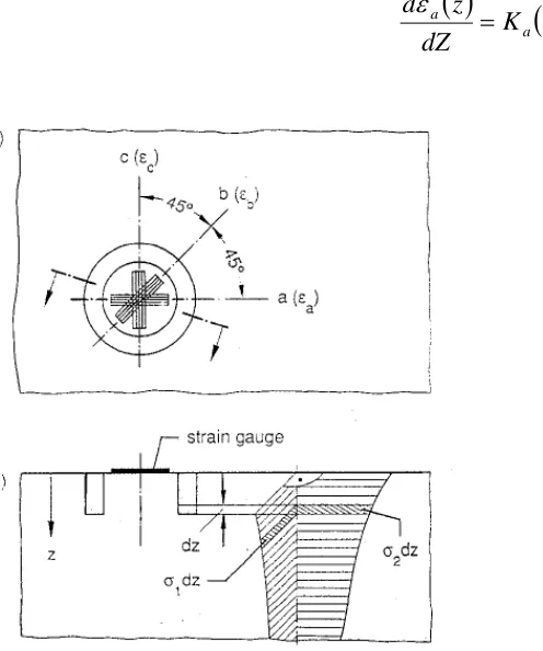
Instead of drilling a hole in the centre of a strain gauge rosette an annular groove is made around a special strain gauge rosette. The resulting strain relaxation is measured on the surface of the cylindrical core. Figure 1 shows the geometry of a strain gauge rosette and the placement of the rosette in relation to the groove. The maximum depth of the groove is dependent on the dimensions specified for the core.
THEORETICAL SOLUTIONAL
amount of dz from its original depth z. The prevailing stress are marked by
σ
a,b,c,d and the relieved strains aremarked by
d
ε
a,b,c,d.. The three strain gauges are in directions a, b and c, direction a is perpendicular to thedirection c and b is perpendicular to direction d. the highest principal stress is
σ
1and it is oriented at angleα
to gauge a., b and c are oriented at angles to each other. In general, the change in strain recorded by gauge a can be described as a function of the depth z by the equation:0 , 45 ,90
D D D( )
( )
)
(
*z
z
K
dZ
z
d
a a
a
ε
ε
=
(1)Fig. 2: Relationship between strains measured on the surface and released stresses in depth Z
Fig. 1: (a) Ring core and strain gage rosette grids (b) Principal stresses and their distribution
In Eq.(1),
K
a(z) is the relaxation function, which describes the effect the strainε
*
a(
z
)
has on the strain gauge for increasing depth z. The relaxation function is dependent on the core diameter, the shape of the groove bottom, the strain gauge and the residual stress state. The relaxation functions can be derived from strain gauge measurements carried out on test specimens that are under a known stress or computationally with finite element analysis, Konig et al. [3].The results fromthe finite element analysis are then verified with previously mentioned measurements on test specimens.The principal stresses
σ
1and
σ
2 can be calculated from the relaxation functions parallel to the principal stresses and the measured changes in strainsd
ε
1/
dx x and d
( )
ε
2/
dx x
( )
. Eq.(2a and 2b) show this dependence, Wolf et al. [4].⎥⎦
⎤
⎢⎣
⎡
+
−
=
dx
x
d
x
K
dx
x
d
X
K
X
K
X
K
E
(
)
)
(
)
(
)
(
)
(
)
(
2 2
1 1
2 2 2 1
1
ε
ν
ε
ν
⎥⎦
⎤
⎢⎣
⎡
+
−
=
dx
x
d
x
K
dx
x
d
X
K
X
K
X
K
E
(
)
)
(
)
(
)
(
)
(
)
(
1 2 2 1 2 2 2 1 2ε
ν
ε
ν
σ
(2b)In Eq.(2a and 2b) E is the modulus of elasticity and
ν
is Poisson’s ratio of the material under study. The directions of the principal stresses are, in general, unknown and the strains are recorded from arbitrary directions a, b, c and d. it can easily be shown based on Mohr’s circle representation that mutually perpendicular stresses and strains correlate with each other as is shown by Eq.(3a and 3b) Gripenberg et. al. [6]):
σ
a+
σ
c=
σ
b+
σ
d=
σ
1+
σ
2 (3a)d
ε
a+
d
ε
c=
d
ε
b+
d
ε
d=
d
ε
1+
d
ε
2 (3b)and that the relaxation functions in directions a,b,c and d are as follows:
K
a(
x
)
=
K
b(
x
)
=
K
1(
x
)
(4a)K
c(
x
)
=
K
d(
x
)
=
K
2(
x
)
(4b)By solving
d
ε
dfrom eq.(3b) and taking eqs (4a) and (4b) into consideration the stresses in directions a, b and c can be calculated with equations (5a),(5b) and (5c):⎥⎦
⎤
⎢⎣
⎡
+
−
=
dx
x
d
x
K
dx
x
d
X
K
X
K
X
K
E
x
a ca
)
(
)
(
)
(
)
(
)
(
)
(
)
(
2 1 22 2 1
ε
ν
ε
ν
σ
(5a)⎥
⎦
⎤
⎢
⎣
⎡
⎟
⎠
⎞
⎜
⎝
⎛
−
+
+
−
=
dx
x
d
dx
x
d
dx
x
d
x
K
dx
x
d
X
K
X
K
X
K
E
x
b a b cb
)
(
)
(
)
(
)
(
)
(
)
(
)
(
)
(
)
(
2 1 22 2 1
ε
ε
ε
ν
ε
ν
σ
(5b)⎥⎦
⎤
⎢⎣
⎡
+
−
=
dx
x
d
x
K
dx
x
d
X
K
X
K
X
K
E
x
c ac
)
(
)
(
)
(
)
(
)
(
)
(
)
(
2 1 22 2 1
ε
ν
ε
ν
σ
(5c)In Eq.(5a, 5b and 5c), the numerator of the parenthetical expression has two separate points where it has a value of zero. The first point is on the surface where z=0 and, therefore,
K
1=
K
2=
0
and the second is deeper and it is zero when the Poisson’s ratio and constants have specific values. This fact limits the use of (5a), (5b) and (5c). In practice the equations are applicable in depths that are reached with current machining methods. With the three stress components calculated the principal stresses together with the three stress components calculated the principal stresses together with the principal directions can be calculated from Eq.(6a and 6b). The angle α is calculated with respect to direction a:1,2
[
(
(
)
(
))
2(
(
)
(
))
2]
2
2
2
)
(
)
(
x
x
x
x
x
x
c b a b ca
σ
σ
σ
σ
σ
σ
σ
=
+
±
−
+
−
(6a))
(
)
(
)
(
)
(
)
(
2
arctan
2
1
x
x
x
x
x
c a c a bσ
σ
σ
σ
σ
α
−
−
−
=
(6b)It can be seen from Eq.(5a, 5b and 5c) that the determination of the stress state as a function of depth is possible with the strains measured on the surface, when knowing the relaxation functions . These functions have to be derived experimentally or numerically .The relaxation functions are dependent on the residual stress state in the material and they are sensitive to the shape of the groove. This means that the relaxation functions can be simultaneously dependent on the stress state, measuring device and material in question. When the relaxation
)
(
)
(
2functions are derived experimentally, a uni-axial stress is introduced to the test specimen and the induced strains are measured. Hook’s law is then applied to these stresses which are parallel to the directions of the principal stresses. The test piece has to be stress free because residual stresses add to the external load applied to the specimen. By comparing the measured surface strains and the real principal strains the relaxation functions
can be derive.
)
(
)
(
21
x
andK
x
K
NUMERICAL SIMULATION
The numerical simulation was performed to model the strain response on the surface of the core at different groove depths under the influence of an external load creating a constant stress to the material cross-section. The relaxation functions applicable for the groove geometry under consideration were derived from the calculated strains by solving in Eq.(1). With the relaxation functions the residual stresses can then be calculated from Eq.(5a, 5b and 5c). The magnitude of the external load was selected to limited stress to ensure elastic behaviour of the investigated material by being far enough from the yield point and to keep the specimen dimensions, the load frame dimensions and the force in the tensile test at an acceptable level.
)
(
)
(
21
x
andK
x
K
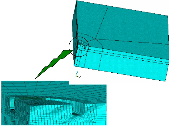
The FE-analysis was based on a specimen volume with dimensions of 250 x 250 x 50 mm3. Due to
symmetry only a quarter was modelled with the centre of the core on the surface as the origin. The elements used were 3-D structural solid. The geometry was well described with this element type without danger of elements interlocking. The details of the FE-model are shown in Fig. 3.
Fig. 3: Finite element view of simulated specimen
The groove depth was increased in steps of 0.25 mm in the simulation. The model was loaded with an external, through the cross-section, constant load of 100 MPa, where the direction of the load action is in the x-direction and the growth of the groove is in the z-x-direction. The elastic modulus used was 210 GPa and the Poisson’s ratio was 0.3. The strains were collected on the surface (x-y-plane) of the core from the origin to a distance of 3.0 mm in the directions 0º and 90º for every calculation step. The strain distribution in each gage direction was established as a function of groove depth starting from the origin (z = 0).
every groove increment. In an accurate analysis the total strain is obtained by integrating over the grid area because in the actual strain gage the strain is measured over the whole measurement grid. The strain derivatives and
0
/
d
ε
dz
andd
ε
90/
dz
were calculated from the simulation which combined with Eq.(1) gave the relaxation functions and . Fifth order polynomials were fitted to the discrete changes of the strains with the least square method.1
( )
K z
K z
2( )
RESULTS AND DISCUSSIONS
Case 1: Uniaxial State of Stress
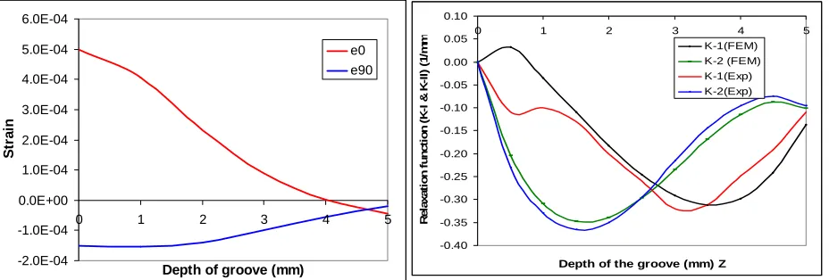
The strains obtained from the simulation using uniform uni-axial stress (100 MPa) on the sides are presented in Fig. 4. The relaxation functions and were calculated form the measured strains with the same procedure as in the FE-analysis. Experimentally obtained relaxation functions from literature and functions obtained by FE-analysis are shown in Fig. 4. The relaxation function
1
( )
K z
K z
2( )
2
( )
K z
from the FE-analysis is not represented correctly at groove depths less than 1 mm due to the mathematical formulation in the fitting procedure. However, the resulting error is negligible, because the influence of the transverse relaxation function on the calculated principal stress is minor at shallow groove depths.-2.0E-04 -1.0E-04 0.0E+00 1.0E-04 2.0E-04 3.0E-04 4.0E-04 5.0E-04 6.0E-04
0 1 2 3 4 5
Depth of groove (mm)
St
ra
in
Case 2: Biaxial State of Stress
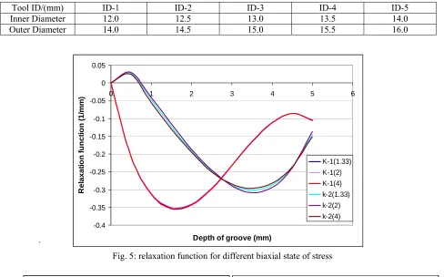
Biaxial state of stress (ratio 1.33, 2.0 & 4.0) has been applied in the simulation and consider same geometry and other parameter as case 1. Relaxation functions
K z
1( )
andK z
2( )
were calculated from the measured strains with the same procedure as in the FE-analysis and presented in the Fig. 5. It was observed for the all biaxial ratio there was close agreement of relaxation function obtained through uniaxial state of stress.Case 3: Effect of Tool Geometry
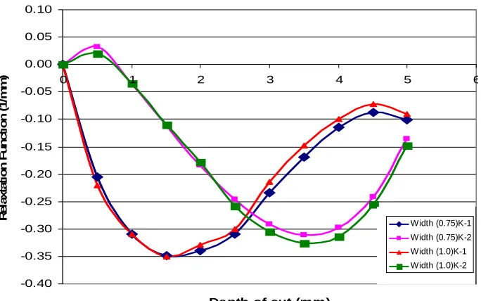
In this case study, different tool geometry consider for evaluating change in relaxation function. Process parameter and simualtion methodology same as case 1. Tool configuration was described in table 1. Relaxation functions for these IDs are shown in Fig. 6. It was observed lower the inner diameter with constant tool thickness lower the relaxation function. Fig. 7, showed the effect of tool thickness on relaxation functions. It was observed lower the tool thickness with constant inner diameter lower the relaxation function.
Fig 4. (a) Relieved strains for uniaxial stress state (b) Comparison of relaxation function
e0
e90
-0.40 -0.35 -0.30 -0.25 -0.20 -0.15 -0.10 -0.05 0.00 0.05 0.10
0 1 2 3 4 5
Depth of the groove (mm) Z
R
e
la
x
a
ti
on f
unc
ti
on (
K
-I
&
K
-I
I)
(
1
/m
m K-1(FEM)
Table 1: Variation in tool geometry
Tool ID/(mm) ID-1 ID-2 ID-3 ID-4 ID-5
Inner Diameter 12.0 12.5 13.0 13.5 14.0
Outer Diameter 14.0 14.5 15.0 15.5 16.0
.
-0.4 -0.35 -0.3 -0.25 -0.2 -0.15 -0.1 -0.05 0 0.05
0 1 2 3 4 5 6
Depth of groove (mm)
R
e
la
x
a
tio
n
fu
n
c
tio
n
(1
/m
m
)
K-1(1.33) K-1(2) K-1(4) k-2(1.33)
k-2(2) k-2(4)
Fig. 5: relaxation function for different biaxial state of stress
-0.35 -0.30 -0.25 -0.20 -0.15 -0.10 -0.05 0.00 0.05 0.10
0 1 2 3 4 5
Depth (mm)
K
-1(
1/
m
m
) ID-1
ID-2 ID-3 ID-4 ID-5
-0.40 -0.35 -0.30 -0.25 -0.20 -0.15 -0.10 -0.05 0.00
0 1 2 3 4 5
Depth (mm)
K-2(1/
m
m
)
ID-1 ID-2 ID-3 ID-4 ID-5
CONCLUSIONS
This paper has provided a systematic study of relaxation function for residual stress measurement by semi destructive ring-core method. The aim of this study was to analyze calibration coefficients K1and K2, which are
necessary for an analytical evaluation of principal residual stresses acting in every drilled layer of examined specimen. The relaxation functions derived in the literature part have maximum situated at a shallower groove depth than in simulation. The strain response in the experiment is sensitive to misalignments at shallow depths. The induced residual stresses from the preparation of the measuring point, i.e., grinding the surface for the application of the strain gage can be significant at the first measuring step. These studies also help us for understand the influence the strain gauge rosette misalignment and tool geometry configuration to evaluate the residual stress using simulation.
REFERENCES
[1] Schajer, G. S. & Roy, G. & Flaman, M. T. & Lu, J., “Hole-Drilling and Ring-Core Methods”, Handbook of Measurement of Residual Stresses, Lilburn, GA 1996, The Fairmont Press Inc. pp. 5-34.
[2] Keil, S., “Experimental Determination of Residual Stresses with the Ring-Core Method and an On-Line Measuring System.”, Experimental Techniques Vol. 16, 1992, pp. 17-24.
[3] König, G., “Ein Beitrag zur Weiterentwicklung teilzerstörender Eigenspannungsmessvervahren”, Doctoral Thesis, Staatliche Materialprüfungsanstalt (MPA), Universität Stuttgart 1991.
[4] Wolf, H. Böhm, Das, W., “Ring-Kern-Vervahren zur Messung von Eigenspannungen und seine Anwendung bei Turbinen und Generatorwellen”, Arch. für Eisenhüttenswesen Vol. 3, 1971, pp. 195-200. [5] Thomas, S., “Contribution to residual stress in isotropic, anisotropic, as well as non homogenous layered
substance using the Hole Drilling Method and Ring Core Method”, Doctoral Thesis, Stuttgart, 1996. [6] Siiriainen, J., Gripenberg, H., and Hanninen, H., “Design and implement of Ring-Core method for residual
stress measurement”.
Fig. 7. Relaxation function for different tool thickness
-0.40 -0.35 -0.30 -0.25 -0.20 -0.15 -0.10 -0.05 0.00 0.05 0.10
0 1 2 3 4 5 6
R
e
la
xt
at
io
n Fu
nct
io
n (
1/
m
m
)
Depth of cut (mm)