Development of Simplified 1D and 2D Models for Studying a PWR Lower Head Failure under Severe Accident Conditions

(1)

18th International Conference on Structural Mechanics in Reactor Technology (SMiRT 18) Beijing, China, August 7-12, 2005 SMiRT18-P01-6

DEVELOPMENT OF SIMPLIFIED 1D AND 2D MODELS

FOR STUDYING A PWR LOWER HEAD FAILURE

UNDER SEVERE ACCIDENT CONDITIONS

V. Koundy, J. Dupas, H. Bonneville

IRSN-DSR

Service d'évaluation des accidents graves et des rejets radioactifs

B.P. 17 – 92262 Fontenay-Aux-Roses Cedex, France

Phone: (33) 1 58 35 74 12, Fax: (33) 1 46 57 22 74

E-mail: [email protected]

I. Cormeau

CS-SI

1 avenue Newton

92142 Clamart Cedex, France

ABSTRACT

In the study of severe accidents of nuclear pressurized water reactors, the scenarios that describe the relocation of significant quantities of liquid corium at the bottom of the lower head are investigated from the mechanical point of view. In these scenarios, the risk of a breach and the possibility of a large quantity of corium being released from the lower head exist. This may lead to direct heating of the containment or outer vessel steam explosion. These issues are important due to their early containment failure potential.

Since the TMI-2 accident, many theoretical and experimental investigations, relating to lower head mechanical behaviour under severe thermo-mechanical loading in the event of a core meltdown accident have been performed. IRSN participated actively in the one-fifth scale USNRC/SNL LHF and OECD LHF (OLHF) programs. Within the framework of these programs, two simplified models were developed by IRSN: the first is a simplified 1D approach based on the theory of pressurized spherical shells and the second is a simplified 2D model based on the theory of shells of revolution under symmetric loading. The mathematical formulation of both models and the creep constitutive equations used are presented in detail in this paper. The corresponding models were used to interpret some of the OLHF program experiments and the calculation results were quite consistent with the experimental data.

The two simplified models have been used to simulate the thermo-mechanical behaviour of a 900MWe pressurized water reactor lower head under severe accident conditions leading to failure. The average transient heat flux produced by the corium relocated at the bottom of the lower head has been determined using the IRSN HARAR code. Two different methods, both taking into account the ablation of the internal surface, are used to determine the temperature profiles across the lower head wall and their effect on the time to failure is discussed. Using these simplified models, a graph representing the time to failure as a function of the pressure level and the heat flux intensity has been determined; such information will be used in our probabilistic safety assessment and severe accident management analyses. Another motivation for the development of simplified models in IRSN is to obtain a simplified but well-predicting code that can then be integrated into integral severe accident computer codes.

(2)

In the event of a severe accident causing a pressurized water reactor (PWR) core meltdown, a large quantity of liquid corium can relocate at the bottom of the reactor pressure vessel (RPV) lower head and generate local heating. This local overheating can lead to a lower head breach resulting in the release of a large quantity of core material into the containment. The size of the breach is important because it defines the conditions of corium ejection. Consequently it is one of the essential parameters required to predict the resulting outcome of the RPV lower head failure, the subsequent ex-vessel accident events and the possible loss of integrity of the containment.

Over the last ten years, IRSN has taken part in the one-fifth scale experimental USNRC/SNL lower head failure programs, in particular in the OECD lower head failure (OLHF) program from 1999 to 2002 (Chu et al., 1999). On the one hand these experiments provided data for model developments and validation, and on the other hand they have lead to a better understanding of the mechanical behaviour of the reactor vessel lower head; both of which are of importance in severe accident assessment and the definition of accident mitigation strategies. In these experiments, particular attention was paid to the timing, mode and size of the breach. The ability to extrapolate the size of the breach to the case of a real reactor is useful and essential for our Level-2 probabilistic safety assessment (PSA) analyses relating to 900MWe PWRs.

In the framework of the OLHF program, three numerical models have been developed by IRSN. The first model, not presented here, deals with 3D finite element modelling. Its development is a current joint research project between IRSN and CEA; the principal objective is to study the evolution of the breach until its final size. The second model is a simplified 1D approach based on the theory of spherical shells subjected to internal pressure and temperature. The third is a simplified 2D model based on the theory of shells of revolution under symmetric loading.

The aim of this paper is to present the two simplified models. Their analytical equilibrium equations, and the creep constitutive equations used are presented. These two simplified models have already been used to interpret some of the one-fifth scale USNRC/SNL experiments. Their results were then compared to the experimental data, as well as to the numerical results that were determined from our OLHF program partner 2D and 3D finite element codes. The numerical results were presented in the Benchmark calculations based on the OLHF1 test (Nicolas et al., 2003; Koundy et al., 2005; Koundy and Cormeau, 2005). These comparisons will not be referred to here, but we say that quite a good agreement between all the calculations and experimental data was obtained.

In this paper, an example of the application of both simplified models to the case of a real reactor will be presented. It has been assumed that the RPV lower head is under severe accident conditions with relocation of corium at its bottom. The average transient curves of the heat flux, which depend on the volume of corium present in the lower head, have been determined by the IRSN HARAR code. Two different methods both of which take into account the ablation of the internal surface, have been used to determine the corresponding temperature profiles across the vessel wall and their effect on the time to failure. Using the two simplified models, a graph giving the time to failure of the lower head as a function of pressure and heat flux intensity has been determined. This graph is required in our Level-2 PSA studies.

The aim of the simplified model development within IRSN is to obtaina simplified but well-predicting code that can then be implemented in the European integral severe accident computer code ASTEC and in the IRSN ICARE/CATHARE code.

2. SEVERE ACCIDENT LOADING CONDITIONS

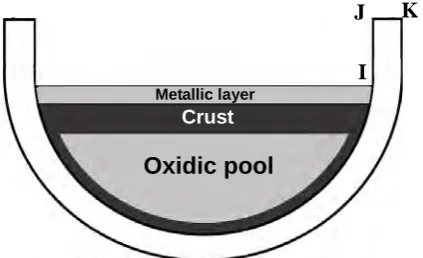
It is supposed here that the relocation of molten corium in the lower head leads to a configuration as illustrated in Fig. 1. In the analysis, major assumptions made are as follows: the debris bed is segregated into an oxidic pool with an overlying metallic layer. The molten oxidic pool is surrounded by an upper crust at the upper surface and a lower crust separating the RPV wall from the pool. No crust is formed between the RPV wall and the overlying metallic layer. These debris bed configurations are the same ones as those used by several authors (Theofanous et al., 1994; Henry and Suh, 1994; Kymalainen et al., 1997).

(3)

Fig. 1. Schematic of melt pool structure in the lower head.

These heat transfer coefficients together with all general properties commonly used for the corium were implemented in the IRSN HARAR code by Bonneville (2002). In our mechanical calculations, only the average transient heat flux from the oxidic pool was used; that resulting from the metallic layer was not taken into account due to the uncertainties concerning the metallic layer thickness and the boundary conditions at the free surface. The IRSN HARAR code enables us to calculate the average transient heat flux and an example of such transient heat flux curves is shown in Fig. 2. In the same figure, a constant heat flux curve associated with the transient curve is plotted; it can be determined simply using the mass of the considered relocated corium, the present mass of uranium oxide, the heat exchange coefficients and the residual power of the core. Theoretically, the heat flux transient curve and its associated constant heat flux curve should lead to approximately the same time to failure of the lower head (equivalent thermal energy applied to the vessel for the same quantity of corium and for a sufficiently long time).

Given that the calculations of time to failure of the RPV vessel using the complete form of the transient heat flux curves are very long and this is not attractive for our Level-2 PSA parametric calculations, the corresponding constant heat flux curves have been used instead of the time-dependent curves.

One can justify experimentally that the value of the heat flux at the upper surface is approximately 1.5 times the value supplied by that in the Fig. 2; the value then decreases to a coefficient close to 0.3 at the pole of the lower head (Seiler and Froment, 2000).

Time (s)

0 10x103 _20x103 _30x103 _40x103

H

e

a

t flu

x

(w

/m

2 )

0 50x103

100x103

150x103

200x103

250x103

300x103

1. Transient Flux 2. Constant Flux

1

2

Fig. 2

.

Transient heat flux from the oxidic pool for a representative case.

The results of our Level-2 PSA parametric calculations concerning 900 MWe PWRs show that the heat flux values range from 20000 W/m2 to 220000 W/m2. The minimum value of the heat flux corresponds to a late flow of corium into the lower head with low residual power and small quantity of relocated molten core material close to 20 tons. The maximum value corresponds to a higher mass of molten core material of approximately 60 tons with high residual power. The relative internal pressure varies from 0.5 105 Pa to 165 105 Pa. The minimum pressure corresponds to the almost complete depressurization of the lower head and the maximum value corresponds to the highest possible pressure in the vessel just before automatic opening of the presurizer safety valves.

3. CREEP CONSTITUTIVE EQUATIONS

The Norton type constitutive creep law has been implemented in the simplified models and defined by the following equation:

Oxidic pool

Metallic layer

Crust

J

(4)

) T ( n ) T ( m eq t

) T ( C

q= σ (1)

where σeq is the von Mises equivalent stress, C(T), m(T) and n(T) are temperature dependent material parameters.

These parameters can be obtained from two databases.

The first is the Sandia database which was developed for SA533B1 steel (Chu et al., 1999). In this database, the exponent n(T)of time has been taken as unity, thus the equivalent viscoplastic strain rate is given by:

) T ( m eq

) T ( C

q= σ (2)

The fitting method used to determine the parametersC(T) and m(T) was presented in detail by these authors and won't be repeated here.

The second database deals with 16MND5 steel which has been used for French PWRs. The parameter n(T) is different from unity (n(T)≠1) and the equivalent strain rate is written as:

(

)

n(T) 1 0 ) T ( m eq t t )

T ( C ) T ( n

q=

σ

− − (3)

where t0 is the time at the onset of creep.

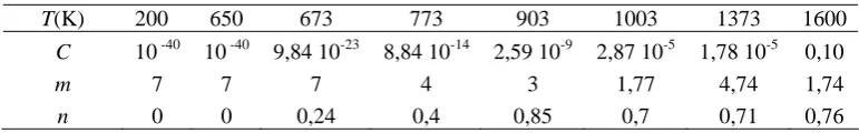
In this paper, an application to the case of a French PWR reactor will be shown and only the strain rate formula given by (Eq. 3) will be employed. The equivalent stress and the time t are expressed in MPa and hours, respectively. In our calculations, it is supposed that creep only occurs when the temperature of the vessel inner surface reaches 670 K. The strong temperature dependence creep parameters used in our calculations are given in Table 1.

Table 1 Creep parameters as a function of temperature

4. SIMPLIFIED MODELS

The detailed descriptions of the simplified 1D and 2D models, including the methods used to determine the temperature profiles across the vessel thickness as well as the theoretical formulations are presented below.

4.1 Simplified 1D model

The simplified 1D model assumes that the lower head is a perfect sphere whose deformation always remains spherical.

4.1.1 Temperature profile calculation

The mesh used in the thermal calculation is a series of twenty-node hexahedra through the lower head wall thickness and the temperature profile is thus determined along these aligned hexahedra.

The temperature profile across the wall is calculated using the general finite element CAST3M code (2004). The thermal method (1Dt-FE) used in this code is that proposed by Dupont et al. (1974) and also presented by Dalhuijsen and Segal (1986). The heat transfer equations were solved using the following boundary conditions: the known heat flux was applied on the vessel inner surface, convection was applied on the vessel outer surface and an adiabatic condition was applied on the remaining surfaces of the model. The convection coefficient used in our calculations is a function of temperature as given in Table 2.

Table 2

Convection coefficient as a function of temperature

During the calculation, the temperature of the lower head inner surface can exceed the melting temperature. From the calculated temperature profile, we can then deduce the thickness of the molten section, as well as the remaining solid section which is necessary for the mechanical calculation. To determine the thickness of the molten section, the 1D mesh needs to be sufficiently refined and more than one hundred elements are used through the wall thickness.

T(K) 200 650 673 773 903 1003 1373 1600

C 10 -40 10 -40 9,84 10-23 8,84 10-14 2,59 10-9 2,87 10-5 1,78 10-5 0,10

m 7 7 7 4 3 1,77 4,74 1,74

n 0 0 0,24 0,4 0,85 0,7 0,71 0,76

T (K) 373 920 960 1040 1480 1600

(5)

The theory of the mechanical calculation used in the simplified 1D model is presented below. An incremental algorithm has been used and for each time step tn+1 the operations below are performed; the time tn+1 is defined by

t t

tn+1 = n+

Δ

where tn is the previous time andΔt isthe time-increment:

- Reading of the profile temperature, update of the solid wall thickness es (after removal of the ablated part).

- Calculation of the von Mises equivalent stress using the membrane theory relating to a sphere with a mean radius R

and subjected to an internal pressure P:

s eq

e 2

PR =

σ

(4)

- Calculation of the equivalent strain rate using Eq. (3) and of the strain increment

Δ

q=q

Δ

t. - Update of the cumulated strain q_n₊₁ =q_n +

Δ

q.

- Stopping the calculation when the failure criterion is satisfied or otherwise repeating the same operation for the next time step.

4.1.3 Failure criteria

Two failure criteria have been used in the calculations. The first one assumes that the lower head failure occurs when the cumulated strain reaches 10% and the second assumes that failure occurs when the following condition is met:

fail eq

σ

≥ where the critical stress

σ

fail is material and temperature dependent and is given in Fig. 3. In this paper

these failure criteria will be called "excessive creep" and "plastic instability", respectively.

16MND5 steel

Temperature (K)

0 150 300 450 600 750 900 1050 1200 1350 1500 1650

Cri

tical s

tress

(MPa)

0 50 100 150 200 250 300 350 400 450 500 550 600 650

Fig. 3. Critical stress as a function of temperature.

The thickness-averaged value of the critical stress has been used in the calculation and this is obtained using numerical integration with 10 segments across the wall thickness.

4.2 Simplified 2D model

The lower head under studyis considered as a thick hemispherical shell with a completely fixed edge condition, subjected to the simultaneous action of a uniform internal pressure and a significant thermal loading caused by the liquid corium relocated at its bottom. The deformation of the lower head is assumed to be caused mostly by creep and to remain axisymmetric until failure; the elastic and thermal deformations are assumed to be negligible.

4.2.1 Equilibrium equations

The model is based on the equilibrium equations of shells of revolution under symmetric loading. By using the local three orthogonal axes at the current point P of the shell middle surface, i.e.:

- the tangent to the parallel of the shell, - the tangent to the meridian of the shell, - and the normal to the shell surface,

(6)

Fig. 4. Definition of variables. Fig. 5. Stress resultants.

In the general case, three equilibrium equations must be satisfied:

(

xN

)

N r cos xQ xr P 0

d d

t 1 1

1

2 − ψ − + =

ψ (5)

( )

)P 0

2 e r ( ) sin 2 e x ( Q x d

d sin r N N

x ₂+ ₁ ₁ + − − ψ ₁− _n=

ψ

ψ (6)

(

xM

)

M r cos xr Q 0

d d

1 1

1

2 − ψ − =

ψ (7)

The first two equations correspond to the force equilibrium in the directions of the tangent (index t) and the normal (index n) to the meridian, respectively. The third equation defines the equilibrium of the moments. N1, N2, M1and M2

are the stress resultants per unit length, Q is the transverse shear force and e is the current shell wall thickness. The normal pressure Pn is assumed to be applied on the inner surface of the shell and therefore the term e2sin

ψ

appears in

Eq. 6. The tangential load Pt is equal to zero in the present case. All radii are defined from the origin to the middle

surface of the shell wall. The problem is assumed to be a membrane-dominated case and thus Eq. 7 won't be taken into account in the present study.

The force equilibrium equation (Eq. 6) in the direction of the normal to the meridian can also be easily established by using the equilibrium of the cap O'PO'' which is the bottom part of the lower head delimited by the horizontal plane O'P. This cap is subjected to an internal pressure p (equal to Pn) and to its dead-weight Wo' as shown in Fig. 6.

Fig. 6. Equilibrium of the Fig. 7. Connection between initial

cap O'PO''. and deformed shell variables.

Written at point P and using the force resultants projected on the Z axis, the equilibrium of this cap can be expressed by:

(

)

o'

2

2 sin ) W

2 e x ( p cos Q sin N x

2 π ψ + ψ = − ψ + (8)

Notice that the pressure p in Eq. 8 is a follower force: it remains always perpendicular to the shell surface. The dead-weight of the spherical cap is given by:

g ) sin 1 ( ) 12 e R ( e 2 W

2 0 2 0 0 '

o = π + − ϕ × ρ (9)

where e0 is the initial thickness of the shell, R0 is the initial radius, ϕ is the polar angle on the undeformed spherical

cap (Fig. 7) and ρg is the specific weight.

From Eq. 8, we can deduce the stress resultant N2as a function of the transverse shear force Q: X Z

P0

R0

ϕ

θ

r 0 X

O'' Z

O'

P

Ψ

θ

Pn

Pt

r1

r

x 0

M1

N2

N1 M2

Q _x

Ψ _Ψ

P

Q

N2

x O'

O''

Pn

Wo'

(7)

N₂ = − 2+ o' − (10)

Substituting Eq. 10 into Eq. 5 and knowing thatx=rcosθ, the stress resultant N1 can be also calculated as a function of Q: ⎟⎟ ⎠ ⎞ ⎜⎜ ⎝ ⎛ − − ⎟⎟ ⎠ ⎞ ⎜⎜ ⎝ ⎛ + − ⎟⎟ ⎠ ⎞ ⎜⎜ ⎝ ⎛ − ⎟ ⎠ ⎞ ⎜ ⎝ ⎛ − = ψ θ θ ψ θ ψ ψ ψ θ ψ θ d d sin r d dr cos sin r Q d dQ N sin r cos r r 2 e sin r cos r 2 e r p N 1 2 1 1 1 1

1 (11)

The expressions of N1 and N2 as given by Eqs. 10 and 11 then depend on:

• the transverse shear force Q which vanishes by symmetry at the pole while its value is not negligible at the edge of the lower head (far from the rupture site),

• the relationship between the polar angleθ on the deformed capand the inclination angle ψ of the meridional about the horizontal plane (Figs. 6 and 7).

Besides, we can say that the vessel failure has taken place after an important viscoplastic membrane creep and we can legitimately suppose to a first approximation that the membrane stresses are appreciably uniform in the thickness in the area of interest, and that the bending moments are negligible in the major parts of the shell. This assumption is in agreement with the observations made on the failure test vessels in the LHF and OLHF programs and it should be re-examined in the zone subjected to a strong thermal gradient.

We will use the following notation hereafter:

4 p 3 ) ( 2 p e Q 2 p e N e N 2 2 2 1 2 1 2 2 2 1 eq 3 2 2 1 1 + + + + − + = = − = = = τ σ σ σ σ σ σ σ τ σ σ σ (12)

the hoop and meridional stresses, the normal stress, the shear stress and the von Mises equivalent stress, respectively.

3

σ and Q are supposed here independent of the creep law. These mean true stress components will be completely determined when the transverse shear force Q is known.

The first approximation chosen in this simplified 2D model uses the Rabotnov formula which gives an explicit approximate analytical expression of the transverse shear force Q, in the case of a thin hemispherical shell under internal pressure. This formula is completely satisfactory for the major part of the shell, except at the pole (Timoshenko and Woinowsky-Krieger, 1959). We introduced a corrective term into this formula to remove this restriction and the final expression of Q used is as follows:

) R e 2 cos( cos e 2 ) 1 ( R p ) ( Q 2 0 0 0 ϕ π ϕ λϕ λ ν ϕ λϕ − −

= − (13)

with 4 / 1 2 0 0 2 ) ) e / R ( ) 1 ( 3 ( ν

λ= −

and

2

0 0

R e

2 _ϕ

π = corrective term

ν is Poisson's ratio which is chosen equal to ½ (this value is generally used when creep predominates over elastic strains).

4.2.2 Numerical integration scheme in the shell thickness

The stress components as well as the equivalent stress defined in Eq. 12, have their values determined at the shell middle surface and are supposed to be uniform in the shell thickness. It has been seen in the OLHF experiments that the stress is lower at the vessel inner surface than at the outer one, which is due to the very temperature sensitive creep mechanical property, especially when the temperature of the heated inner surface is close to the melting temperature.

The equilibrium equations (Eqs. 5 and 6) that are written using the membrane stress resultants per unit length and not the local stresses, cannot be used then to solve the problem of local stress variation in the vessel thickness. Therefore, an additional hypothesis which is of prime importance in this simplified 2D method is adopted and assumes that, at any point of the shell middle surface, the equivalent strain rate is uniform in the shell thickness. The equivalent strain rate is connected to the viscoplastic tensor by:

eq p q 2 3 σ σ

ε = ′ (14)

(8)

Substituting Eq. 2 into Eq. 14 (the same proof holds for Eq. 3), the principal components of the strain rate at any local point in the vessel thickness can be expressed as:

⎪ ⎭ ⎪ ⎬ ⎫ ⎪ ⎩ ⎪ ⎨ ⎧ = ⎪ ⎭ ⎪ ⎬ ⎫ ⎪ ⎩ ⎪ ⎨ ⎧ − 3 2 1 1 m eq 3 2 1 s s s 2 C 3 σ ε ε ε (15)

where S1, S2 and S3 denote the deviatoric stresses in the azimuthal, meridional and radial directions, respectively.

The equivalent strain rate is given by:

(

)

(

)

m

eq 2 3 2 2 2 1 1 m eq 2 3 2 2 2 1

eq s s s C

2 3 C

3

2 _ε _ε _ε _σ _σ

ε = + + = − + + = ₍₁₆₎

The above additional hypothesis assumes that ε_eq must be constant at any point across the wall thicknesssince no significant bending appears, hence the following system of equations can be established:

( )

_{( )}

( )

₍

₎

1 L i 1 cst ) T ( C ) T (

C ξ_i σ_eq ξ_i m(Tξi ) = ξ_L σ_eq ξ_L m(TξL ) =ε_eq = ≤ ≤ − ₍₁₇₎

where ξ1,ξ2,...ξLdenote the L Lobatto sampling points, used to carry out numerical integration across the wall

thickness (Stroud and Secrest, 1966). The material parameters C and m calculated with the temperature at the pointξi

and the equivalent stress σeq calculated at the point ξi will be denoted by Ci, miand σeq( )i to ease the notation. With

these notations, Eq. 17 becomes:

( )

₍

₎

1 L i 1 cst C C eq m L eq L m i eq i L

i ₌ σ ₌ε ₌ _≤ _≤ ₋

σ ₍₁₈₎

The simultaneous equations (Eq. 18) define implicitly the variation of the equivalent stress in the vessel wall, while the variation of the temperature is known across the thickness. As the value of the constant cst is not a priori known and this constant varies in time and with respect to the position considered along the meridian of the shell middle surface, the problem can be solved upon identifying the two following numerical integrals:

(

)

∫

= + − + + + + = e eq 2 2 2 1 2 1 2 2 2 1 eq e 4 p 3 2 p e

de σ σ σ σ σ σ τ σ

σ (19)

( ) ( ) ( )

(

L

)

eq L 2 eq 2 1 eq 1 e

eq w w w

2 e

de σ σ σ

σ = + + +

∫

" (20)

where w1,w2,...wLdenote the weights corresponding to the L Lobatto points.

Replacing into Eq. 20, the expression of σeq( )i (with 1≤i≤L−1) given by Eq. 18, and considering Eq. 19, the

following nonlinear equation for the single unknown σeq( )L is obtained:

( )

( ) eq L eq L 1 L 1 i m m L eq m 1 i L

i w 2

C C w i L i σ σ σ + = ⎟⎟ ⎠ ⎞ ⎜⎜ ⎝ ⎛

∑

− = (21)

Parameters Ci and mi (with1≤i≤L), which depend of the temperature at each Lobatto point, are determined from

the used creep law. The Newton method has been used to solve Eq. 21, whenceσeq( )i (with1≤i≤L−1) as well as εeq

can be deduced from the knownσeq( )L using Eq. 18.

The above method mentioned thus provides a discrete representation of the distribution of the equivalent stress in the wall thickness and the fineness thereof is completely controlled by integer L. Notice that the choice of the above additional hypothesis in this simplified model replaces the nonlinear material stress-strain law that would be used in a finite element model.

4.2.3 Large displacement model

The shell theory presented above, available for a small displacement study, is insufficient to describe the lower head deformation under severe accident conditions. It has been seen in the LHF and OLHF programs that the deformed test vessel sagging could exceed several times the initial vessel thickness. The method of large displacements and large strains, used in this simplified 2D model consists of expressing analytically r

( )

θ and θ

( )

ϕ as follows:

θ β θ α

θ 2 4

0 sin sin

R ) (

r = + + (22)

ϕ ϕ ϕ ϕ ϕ ϕ

(9)

These equations define the connection between initial and ovoid shell variables (Fig. 7). The six parameters α, β,a, b, c

and d make up the six mechanical (displacement-like)degrees of freedom of the simplified 2D model. The choice of the number of parameters here is arbitrary but seems sufficient to correctly describe the shell deformation. We can verify the following boundary conditions, for 0≤ϕ≤π₂ and 0≤θ ≤π₂:

0

R ) 0 (

r = , θ(0)=0 and θ(π2)=π2 (24)

It should be noted that polar anglesϕ andθ are in general different, except at the equator and at the pole of the shell. From analytical surface theory, one can obtain the following matrix system connecting the rate of these parameters to the strain and curvature rates of the shell:

[

]

⎪ ⎪ ⎪ ⎪ ⎭ ⎪⎪ ⎪ ⎪ ⎬ ⎫ ⎪ ⎪ ⎪ ⎪ ⎩ ⎪⎪ ⎪ ⎪ ⎨ ⎧ = ⎪ ⎪ ⎪ ⎭ ⎪⎪ ⎪ ⎬ ⎫ ⎪ ⎪ ⎪ ⎩ ⎪⎪ ⎪ ⎨ ⎧ d c b a ) , e , R ; d , c , b , a , , ( B e 0 0 2 1 2 1 β α ϕ β α κ κ ε ε (25)

The strain rates ε1 and ε2 are determined from the creep law used (Eq. 15). The derivative of the current thickness,

due to the material incompressibility hypothesis, can be given by:

3 2

1 ) e

( e

e=− ε +ε = ε (26)

The kinematic relations and the long analytical calculation of the matrix [B] are not presented here; one can specify that difficult analytical expressions were calculated using Mathematica (Wolfram, 1999).

Numerically, the following geometrical discretization was used: the polar angle ϕ (with0≤

ϕ

≤π₂) was divided into one hundred intervals and twelve Lobatto sampling points were considered across the wall thickness to account for the temperature dependent material properties. The stress was calculated at each Lobatto point by assuming (as mentioned above) that the corresponding equivalent strain rate was uniform across the wall thickness, considering the experimental evidence (as observed in the LHF and OLHF programs) whereby the test vessels experienced very little bending as compared to extension in tension.

4.2.4 Main model system matrix

From the virtual work principle stating that internal and external works are equal whatever the admissible virtual displacements, the following six by six system of ordinary differential equations arises:

[ ]

Γ

{

α β a b c d

}

T =

{ }

F (27)

where the generalized force vector {F} and the generalized damping matrix [Γ] are built from numerical integration

along the meridional curve of analytical expressions provided by the simplified model. The details of the long analytical calculation of the vector {F} are not presented here. The final expression of the damping matrix [Γ] can be given by the

following equation:

[ ]

_∫

[ ]

⎥

[ ]

⎦ ⎤ ⎢ ⎣ ⎡ = 2 0 2 1 2 1 t eq eq 0 2 0 d B 1 1 B 3 cos e R 8 π

ϕ

ε

σ

ϕ

π

Γ

(28)

where

[ ]

B is the matrix [B] of Eq. 25, reduced to the two first components ε1 and ε2. Eq. 28 shows that the

generalized damping matrix [Γ] is symmetric and positive definite.

The problem arising has been solved using an iterative procedure. While the force vector and damping matrix are calculated from known values of parameters α, β, a, b, c and d at step (n), parameters at step (n+1) are updated using the Euler explicit recurrence scheme (with constant or variable time step

Δ

t):

[ ]

{ }

F t

d c b a d c b a n 1 n n n n n n n 1 n 1 n 1 n 1 n 1 n 1 n Δ Γ β α β α − + + + + + + + ⎪ ⎪ ⎪ ⎪ ⎭ ⎪⎪ ⎪ ⎪ ⎬ ⎫ ⎪ ⎪ ⎪ ⎪ ⎩ ⎪⎪ ⎪ ⎪ ⎨ ⎧ = ⎪ ⎪ ⎪ ⎪ ⎭ ⎪⎪ ⎪ ⎪ ⎬ ⎫ ⎪ ⎪ ⎪ ⎪ ⎩ ⎪⎪ ⎪ ⎪ ⎨ ⎧ (29)

(10)

As mentioned above, the use of the complete transient heat flux curve presented in Fig. 2 requires a very long calculation time. This is not practical for our parametrical calculations and this is not compatible with the simplified character of our models which have to provide fast results. Consequently, the use of the corresponding constant heat flux (Fig. 2) seems more suitable. A simplified method considering a constant heat flux has been chosen and was implemented in the simplified 2D model. It supplies an approximatequadratic profile of temperature across the wall thickness. Naturally, more elaborate temperature profiles obtained fromthe finite element method can be used thereafter to validate some calculations or to study the effects on time to failure of this quadratic approximation.It should be noted that this constant heat flux option (implemented in the simplified 2D model) will not be integrated in the general severe accident computer codes; it has been used for experiment interpretation and is only used here for comparing times to failure between our two simplified 1D and 2D models.

The method used to calculate the quadratic temperature profile is described below. The problem of the determination of the transient temperature field in the wall thickness has been reduced to 1D geometry. The heat conduction equation with boundary conditions is as follows:

( )

t x e

0 t T C x T p 2 2 ≤ ≤ = ∂ ∂ − ∂ ∂

_ρ

_ξ

λ

(30)

( )t h corium

x dt

d L x

T

_ρ

ξ

_φ

λ

ξ = + ∂ ∂ − = (31)

( )_t melting

x T

T _=ξ = (32)

(

T T

)

0

h x T env e x e x = − − ∂ ∂ − ₌ =

λ

(33)

Eq. 30 introduces the thermal characteristics of the lower head "λ, ρ and Cp" and the studied domain ranging

between the possible mobile melting front x=

ξ

( )

t and the fixed external wall x=e (Fig. 8). In this approach, these thermalcharacteristics are all assumed constant.

Fig. 8.

Thickness abscissa

Fig. 9.

Approached temperature profile

Eqs. 31 and 32 correspond to the boundary conditions at the melting front, where Lh denotes the latent heat, the heat

flux φcorium is assumed to be constant in time and is prescribed on the inner wall of the lower head and Tmelting is the

melting temperature. Eq. 33 states the boundary condition on the outer wall as a function of the convection coefficient h

and of the lower head external temperature Tenv .These parameters Tenv and h are also assumed to be constant in this

approach. Two initial conditions (at t = 0) are needed and are given by the following equalities:

( )

0 0

e x 0 T 0 , x T env = ≤ ≤ =

ξ

(34)

The temperature profile is interpolated by a parabolic function as shown in Fig. 9 and is defined by:

(

)

(

)

(

)

(

)

⎪ ⎪ ⎪ ⎩ ⎪⎪ ⎪ ⎨ ⎧ ≤ ≤ = ≤ ≤ + − − − + − ⎟⎟ ⎠ ⎞ ⎜⎜ ⎝ ⎛ − − = ≤ ≤ ≤ = e x T T x T x x 4 T T x T x 0 T T T * ext * ext 2 * * ext int 2 * * melting int

ξ

χ

ξ

(35)

ξ

*

ξ

(t ) e

0 x 0 e

(11)

where

(

)

T x _x *

* 4 1 ξ

ξ

χ

₌₋ ₋ ∂ _∂ ₌ _{is related to the slope of the temperature profile at} * x=

ξ

.

We can notice that as long as the lower head inner wall temperature is lower than the melting temperature, many simplifications exist, due to the vanishing of variable

ξ

=0 and its derivative d

ξ

dt=0.

To determine the temperature profile according to Fig. 9, four configurations arise as summarized in Table 3.

Table 3 Four configurations in the thermal model.

ξ = 0 (without ablation) ξ > 0 (with ablation) ξ*

< e

Conf. 01 Tint≤Tmelting

Text = Tenv

χ = 0

Conf. 11 Tint = Tmelting

Text = Tenv

χ = 0

ξ*

= e

Conf. 02 Tint≤Tmelting

Text≥ Tenv

χ≠ 0

Conf. 12 Tint = Tmelting

Text≥ Tenv

χ≠ 0

Configurations 01 and 11 correspond to the temperature pattern without heat flux at the external wall (Text = Tenv)

and configurations 02 and 12 correspond to the opposite case (Text≥ Tenv). Ablation starts when Tint reaches the melting

temperature. The unknowns appearing in each configuration are as follows: - ξ* and Tint in configuration 01,

- ξ* and ξ in configuration 11, - Tint, Text and χ in configuration 02,

- ξ, Text and χ in configuration 12.

Another important point in the solution of the problem is the transformation of the partial differential equation (Eq. 30) into an ordinary differential equation using the method presented by Kantorovich and Krylov (1964) and by Arpaci (1966). This method was also used by other authors (Krajewski, 1975; Kim, 1976; Laura and Cortinez, 1989).

Eq. 30 is integrated over the interval

ξ

≤x≤

ξ

*:

* * * x T dx x T dx t T C ₂ 2 p ξ ξ ξ ξ ξ ξ

ρ

λ

∂ ∂ = ∂ ∂ = ∂ ∂

∫

(36)

Since the first term of Eq. 36 can be expressed as:

( )

t d d T C t d d T C dx T C dt d dx t T C p * * p p p * *

ξ

ρ

ξ

ρ

ξ ξ ξ ξ ∂ = − + ∂

∫

(37)

By identifying Eqs. 36 and 37, we obtain:

( )

_⎟⎟ ⎠ ⎞ ⎜ ⎜ ⎝ ⎛ + ∂ ∂ − ⎟ ⎟ ⎠ ⎞ ⎜ ⎜ ⎝ ⎛ + ∂ ∂ = = =

∫

d_d_t

T C x T t d d T C x T dx T C dt d p x * * p x p * *

ξ

ρ

λ

ξ

ρ

λ

ρ

ξ ξ ξ ξ (38)

By substituting the expression of T (given by Eq. 35) into Eq. 38 and using the boundary conditions defined by Eqs. 31 and 33, we obtain the corresponding ordinary differential equation:

(

)

(

)

(

p int h

)

(

ext env

)

corium

* ext p int ext * p T T h t d d L T C t d d T C 2 T T 2 3 C dt

d

ρ

_ξ

_χ

₌

_ρ

ξ

₋

_ρ

₊

ξ

₋ ₋ ₊

_φ

(12)

Eq. 39 corresponds to the heat balance equation governing the evolution of the enthalpy of the interval e

x

0≤

ξ

≤ ≤

ξ

* ≤ . Finally, the solution of the thermal problem is equivalent to solving Eq. 39 with its initial conditions and boundary conditions, in each of the four configurations mentioned in Table 3. This was done with the assumption that the thermal properties are considered constant, the temperature profile (solution of the thermal problem) can be analytically determined.

Numerically, the lower head generatrix (corresponding to polar angle interval0≤

ϕ

≤π2) was divided into 91

nodes (or 90 intervals) while a temperature profile was calculated at each node. The temperature profile in the wall thickness was defined by 11 Lobatto integration points.

5. NUMERICAL APPLICATION

The simulation of the lower head thermo-mechanical behaviour of a 900MWe pressurized water reactor under severe accident conditions was carried out. The computational procedure is separated into two steps. The first one consists in performing calculations with constant heat flux and a time to failure chart can be drawn. The second step consists in validating the preceding results by considering another series of calculations using transient heat flux. The effect of the simplifying assumption and the ensuing error are presented.

5.1 Calculation data

The French RPV lower head dimensions are considered. The mean radius is about 2 m and the thickness is about 0.135 m. The initial temperature of the lower head is assumed to be equal to 373 K and the melting temperature of the 16MND5 steel is chosen as 1600 K. Other steel properties are given as follows:

- Density (ρ): 7800 kg/m3

- Thermal conductivity (λ): 30 W/m.K - Specific heat (Cp): 650 J/kg.K - Latent heat (Lh): 270000 J/kg

The convection coefficient (h) is assumed constant and equal to 50 W/m2.K in the simplified 2D model and the values given in Table 2 are used in the simplified 1D model.

5.2 Time to failure chart

The lower head time to failure is important in our Level-2 PSA analyses because it is one of the parameters which are used to define the initial conditions for all outer vessel events. It is used as input data for the codes that relate to the modelling of molten core concrete interaction, as well as the modelling of fission product release under accidental conditions.

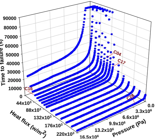
The time to failure chart has been constructed using the simplified 1D model. A series of systematic and parametric calculations, with the constant heat flux values ranging from 20000 W/m2.K to 220000 W/m2.K that were divided into 15 different levels, and with the pressure level ranging from 0.5 105 Pa to 165 105 Pa divided into 185 different levels. The calculations thus include a total of 2257 sets of constant heat flux values and constant pressures. The time to failure chart obtained is presented in Fig. 10.

The set of2257 points in Fig. 10 has been used in a least square fit to obtain the corresponding following mathematical function (time to failure as a function of heat flux and pressure):

( ) ( )

( )

_{( )}

_⎥

⎦ ⎤ ⎢

⎣ ⎡

+ +

=

φ

₂

r

c pressure

b 1

a t

log (40)

where tr is the lower head time to failure, log is the decimal logarithm and the coefficients a, b and c are given by:

( )

9.95110 log

( )

8.64353

a

φ

=− −1

φ

+

( )

6 2

( )

7

( )

7

3 6

4 5 5

4 6

2

10 5753 . 1 log 10 81305 . 1 log

10 61618 . 8 log

10 16004 . 2

log 10 00523 . 3 log

10 19238 . 2 log

10 51859 . 6 b

+ −

=

φ

) 10 31694 . 9 10 85667 . 1 10

237876 . 5 ; 0 ( Max ) (

(13)

0 10000 20000 30000 40000 50000 60000 70000 80000 90000

0.0

3.3x106

6.6x106

9.9x106

13.2x106

16.5x106

44x103

88x103

132x103

176x103

220x103

T

im

e

t

o

f

a

il

u

re

(

s

)

Press ure (P

a)

He at f_lux

(w /m 2

)

C04 C17

C16

C26

Fig. 10.

Time to failure as a function of constant heat flux and constant pressure.

5.3 Comparison of results and discussion

The second step consists in validating these results by performing the same calculations with the simplified 1D model but this time the constant heat fluxes were replaced by their corresponding transient heat fluxes (see Fig. 2). Notice that the constant heat flux defined in Fig. 10 corresponds to approximately 1.5 times the constant heat flux shown in Fig. 2 (this corresponds to the maximum value localized at the melt pool upper surface). As the new calculations became very long, only 91 significant loading sets (p,φ) were selected and plotted as circles in Fig. 11.

These 91 loading sets describe roughly the envelope of all the loading sets used in the first calculation step.

Fig. 11.

Significant loading cases studied in the second calculation step.

In parallel with these 91 new calculations performed with the simplified 1D model (using complete heat flux transient curves), 14 calculations were performed with the simplified 2D model. These additional calculations correspond to the loading sets represented by black dots in Fig. 11.

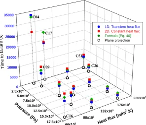
In this paper, the comparison of the results between the models is given only for the last 14 cases mentioned (black dots in Fig. 11). The time to failure as a function of heat flux and pressure, calculated by: (1) simplified 1D model with complete transient heat flux curve, (2) simplified 2D model and (3) using Eq. 40, are plotted in Fig. 12.

Pressure *1E-07 (Pa)

0.00 0.25 0.50 0.75 1.00 1.25 1.50 1.75

He

at Flux *

1e-3

(W/m

2 )

23 46 69 92 115 138 161 184 207 230

C51 C26

C27

C09 C17

C04

C13a C13b

C29a C29b

C45

C16 C61

(14)

0 5000 10000 15000 20000 25000 30000 35000

44x103

88x103

132x103

176x103 220x10 2.5x106

5.0x106 7.5x106

10.0x106 12.5x106

15.0x106 17.5x106

T

im

e

to

f

ai

lure

(s

)

Heat flu x (w/m

2_.K)

Pre ss

ure_(P a)

1D. Transient heat flux 2D. Constant heat flux

Formula (Eq. 40)

Plane projection

Fig. 12

.

Time to failure calculated using the three models.

The detailed analysis of the results between the three models as shown in Fig. 12 leads to the following comments: • For each loading set, the time to failure was obtained for the same failure criterion (either by excessive creep or by

plastic instability) between the simplified 1D and 2D models,

• The times to failure obtained by the three models are comparable. However, we observe that the relative discrepancy increases (when we compare the time to failure calculated by the 2D simplified model withregard to those given by Eq. 40), in particular in the cases of long creep. The maximum relative discrepancy was observed in the cases C04 and C17 and their values are approximately 21% and 20%, respectively. These differences are mainly due to the use of a constant value of h in the simplified 2D model and a variable h in the simplified 1D model (both considered constant heat fluxes).

5.4 2D transient heat flux calculations

In order to compare the time to failure under the same thermal conditions between the simplified 1D and 2D models, two temperature fields were calculated using the two-dimensional thermal (2Dt-FE) calculation option implemented in CAST3M (2004). The mesh used was made up of 900 eight-node quadrilateral elements. The two additional thermal calculations corresponding to the cases C04 and C17 respectively, were performed with the following boundary conditions: the known heat flux was imposed on the vessel inner surface in contact with the pool (Fig. 1), an adiabatic condition was applied on the vessel surface delimited by IJK (see Fig. 1) and a convection condition was applied on the vessel outer surface. The temperature field of the case C04 is presented in Fig. 13.

Fig. 13.

The temperature field at time t=25000 s for case C04.

C04

C17

C16 C09

C51

C26

(15)

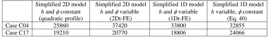
The new comparison between the times to failure obtained by the simplified 2D model using the two-dimensional temperature field calculated by the (2Dt-FE) thermal option of CAST3M, and those obtained from the simplified 1D model is summarized in Table 4; previous results are also included in this Table.

Table 4 Comparison of times to failure (s), between the simplified 1D and 2D

models with different ways of calculating temperatures profiles.

Simplified 2D model

h and φconstant (quadratic profile)

Simplified 2D model

h and φvariable (2Dt-FE)

Simplified 1D model

h and φvariable (1Dt-FE)

Simplified 1D model

h variable,φconstant (Eq. 40)

Case C04 25860 37420 33800 32855

Case C17 19210 20770 18806 24066

With the new thermal field, using a thermal "2Dt-FE" calculation (directly comparable to the thermal "1Dt-FE" calculation), the difference between the two simplified models (columns 3 and 4, Table 4) is approximately equal to 10% for both the C04 and C17 cases. We can see that the time to failure calculated by the simplified 2D model is in general higher than those calculated by the simplified 1D model (with a general relative discrepancy roughly close to 10% or 11%). This remark is consistent with that mentioned by Koundy and Cormeau (2005) which suggests that the 1D model is both overstressed and overheated. These authors have also shown that the time to failure from the simplified 2D model is close to that obtained experimentally and that the time to failure calculated using the finite element codes was between those determined from the simplified 1D and 2D models.

6. CONCLUSIONS

From this work, the following conclusions can be drawn. Lower head failure under severe accident conditions can be studied by simplified models. The simplified 1D model can estimate times to failure (in general about 10% sooner than those calculated by the simplified 2D). The inconvenience of the 1D model is that it supplies other results (stress, strain) in the form of mean values calculated at the mean surface of the wall thickness and cannot give the global behaviour of the lower head like the simplified 2D model. The simplified 2D model is able to describe correctly the global lower head deformation in time (thickness, sagging) and the calculations presented here validate it before its implementation into integrated severe accident computer codes ASTEC and ICARE/CATHARE.

REFERENCES

[1] Arpaci, V. S., (1966), "Conduction heat transfer", Addison-Wesley, Reading, Massachusetts.

[2] Bernaz, L., Bonnet, J. M., Seiler, J. M., (2001), "Investigation of natural convection heat transfer to the cooled top boundary of a heated pool", Nuclear Engineering and Design, Vol. 204, pp. 413-427.

[3] Bonnet, J. M., Seiler, J. M., (1999), "Thermal hydraulic phenomena in corium pools: the BALI experiment", ICONE 7,Tokyo, Japan, April 19-23.

[4] Bonneville, H., (2002), User's manual of HARAR, IRSN/DPEA/SEAC/2002/049.

[5] CAST3M, (2004), General structural analysis code, version 2004, CEA/DM2S, Saclay, France.

[6] Chu, T.Y., Pilch, M.M., Bentz, J.H., Ludwigsen, J.S., Lu, W.-Y., Humphries, L.L., (1999), "Lower Head Failure Experiments and Analyses", NUREG/CR-5582, SAND98-2047.

[7] Dalhuijsen, A. J., Segal, A., (1986), "Comparison of finite element techniques for solidification problems", International journal for numerical methods in engineering, vol. 23, pp. 1807-1829.

[8] Dupont, T., Fairweather, G., Johnson, J. P., (1974), "Three-level Galerkin methods for parabolic equations", Siam, Journal of Numerical analysis, vol. 11 issue 2, pp. 392-410.

[9] Henry, R. E., Suh, K. Y., (1994), "Integral analysis of debris material and heat transport in reactor vessel lower plenum", Nuclear Engineering and Design, Vol.151, pp. 203-221.

[10] Kantorovich, L. V., Krylov, V. I., (1964), "Approximate methods of higher analysis", Wiley, New York, pp. 240-357. [11] Kim, R. H., (1976), "The Kantorovich method in the variational formulation to an unsteady heat conduction", Letters

in heat and mass transfer, vol. 3, pp. 73-80.

[12] Koundy, V., Durin, M., Nicolas, L., Combescure, A., (2005), "Simplified modeling of a PWR reactor pressure vessel lower head failure in the case of a severe accident", Nuclear Engineering and Design, Vol.235, pp. 835-843. [13] Koundy, V., Cormeau, I., (2005), "Semi-analytical modeling of a PWR lower head failure under severe accident

conditions using an axisymetrical shell theory", Nuclear Engineering and Design, Vol.235, pp. 845-853.

[14] Krajewski, B., (1975), "On a direct variational method for nonlinear heat transfer", International journal of heat and mass transfer, vol. 18, Issue 4, pp. 495-502.

(16)

[16] Laura, P. A., Cortinez, V. H., (1989), "An extension of the Kantorovich method and its application to a steady state heat conduction problem", International journal of heat and mass transfer, vol. 32, Issue 3, pp. 611-613.

[17] Nicolas, L., Durin, M., Koundy, V., Mathet, E., Bucalossi, A., Eisert, P., Sievers, J., Humphries, L., Smith, J., Pistora, V., Ikonen, K., (2003), "Results of benchmark calculations based on OLHF-1 test", Nuclear Engineering and Design, Vol.223, pp. 263-277.

[18] Seiler, J.M., Froment, K., (2000), "Interpretation and use of RASPLAV results in support of in-vessel retention", CSNI/NEA RASPLAV Seminar, 14-15 November, Munich, Germany.

[19] Stroud, A.H., Secrest, D., (1966), "Gaussian quadrature formulas", Prentice-Hall, Englewood Cliffs.

[20] Theofanous, T. G., Liu, C., Angelini, S., Kymalainen, O., Tuomisto, H., Addition, S., (1994), "Experiment from the first two integrated approaches to in-vessel retention through external cooling", OECD/CSNI/NEA Workshop on Large Molten Pool Heat Transfer, Grenoble, France, March 9-11.