Article
1
Innovative strategies for bearing lubrication
2
simulations
3
Franco Concli 1,*, Christian Thomas Schaefer 2 and Christof Bohnert 2
4
1 Free University of Bolzano/Bozen; franco.concli@unibz.it
5
2 Schaeffler Technologies AG & Co. KG; christian.schaefer@schaeffler.com, christof.bohnert@schaeffler.com
6
* Correspondence franco.concli@unibz.it; Tel.: +39-0471-017-748
7
8
Abstract: Efficiency improvement is the new challenge in all fields of design. In this scenario the
9
reduction of power losses is becoming more and more a main concern also in the design of power
10
transmissions. Appropriate models to predict power losses are therefore from the earliest stages of
11
the design phase. The aim of the project is to carry on lubrication simulations of several variants of
12
a cylindrical-roller-bearing to understand the lubricant distribution and the related churning power
13
losses. Several strategies to reduce the computational effort have been used. Among them the
14
sectorial symmetry and three innovative meshing strategies (purely analytical with and without
15
interfaces and analytical/subtractive) that have been implemented in the OpenFOAM®
16
environment. The results of the different approaches were compared among them and with
17
experimental observations showing good agreement and reasonable savings in terms of
18
computational effort.
19
Keywords: bearing; lubrication; CFD; OpenFOAM® ; meshing.
20
21
1. Introduction
22
Eco-friendly technologies represent a positive trend for the future. The achievement of ambitious
23
goals in terms of energy savings is strictly related to the capability to design more efficient systems.
24
In these regards, the recent developments in computer science have opened new possibilities.
25
While in the past different design solutions were characterized from an energetic point of view by
26
means of experimental tests, in the recent years more and more numerical studied are available in
27
literature. Numerical techniques, in fact, allow to overcome the need of prototyping, enabling a
28
comparison and an optimization of the different designs starting from the earliest stages of the
29
development.
30
With focus on the efficiency/thermal behavior regarding churning of mechanical components,
31
including bearings, CFD (Computational Fluid Dynamic) seems to be one of the most appropriate
32
tools. Among the different approaches, SPH (Smooth Particle Hydrodynamic), a meshless method,
33
has the advantage of being easily applicable [1] even if the accuracy of the results was proved to be
34
insufficient for comparable computational effort [2][3]. On the other side, mesh-based methods such
35
as FV (Finite Volume) ensure a very high accuracy but in most cases the computational effort required
36
is not compatible with the industrial practice [4]. To partially overcome this problem, in the past
37
several attempts were made. In particular, rotating reference frames [5][6], innovative partitioning
38
strategies [7][8] and, mostly, mesh-handling algorithms [9][10][11][12][13] have been developed and
39
applied in order to reduce the simulation effort.
40
The goal of this research is to study the lubrication and the efficiency of a roller bearing. For this
41
purpose, several levels of geometrical simplifications were introduced. For each model, ad-hoc
42
meshing strategies were developed and implemented in the OpenFOAM® environment. The idea is
43
to try to limit the computational effort by avoiding any kind of mesh deformation and need for
44
remeshing, together with an analytical control of the mesh generation to better handle the element
45
distribution and quality parameters.
46
2. Materials and Methods
47
2.1. Bearing Losses
48
Bearings allow the relative rotation between two mechanical components. They can be classified
49
into two main categories: journal or rolling bearings.
50
In journal or hydrodynamic bearings, the converging gap ensures that the two surfaces are kept
51
separated by a fluid film. To the fluid film are associated the supporting lift forces but also the
52
frictional losses. The power dissipation is mainly due to viscous effects. This kind of bearing was
53
already studied in the past by the author using OpenFOAM® [14]. This kind of simulations is
54
relatively simple from a geometrical point of view because the domain doesn’t significantly change
55
its shape during operation.
56
Rolling bearings carry the load by means of interposed rolling elements. Although also in this
57
case a hydrodynamic film generates in the contacts, the predominant interactions for churning losses
58
are due to the rotation of the cage and motion of the rolling elements. This is the main cause both for
59
the lubricant flow and the losses.
60
The load independent power losses of bearings, in fact, can be classified into seal losses and
61
hydraulic losses. The latter can be further subdivided into squeezing and churning/windage ones.
62
Squeezing losses are mainly related to volume variations and pressure gradients that causes
63
additional flows. Churning losses are due to the splashing of the lubricant due to the motion of the
64
components. It is well known that the squeezing losses, except for spray lubrication, are of a lower
65
order of magnitude with respect to the churning ones [15][16].
66
2.2. Bearing Geometry
67
The bearing considered in this study is a Schaeffler NU222-E-XL-M1/M1A. It is a cylindrical
68
roller bearing which dimensions are listed in table 1.
69
70
Table 1. Parameters of the bearing
71
Dimension Value Parameters Value
d [mm] 110 C0r [kN] 345
D [mm] 200 Cr [kN] 365
B [mm] 38 nG [rpm] 5300
72
This model of non-locating bearing with a single row of cylindrical elements has a very high
73
radial load carrying capacity and is suitable for higher speeds compared to full complement designs.
74
The rollers are guided between rigid ribs in the outer ring. The cage has a solid design and is made
75
of brass. The radial clearance is less than 90 m.
76
77
The lubricant is supplied radially into the space in front of the bearing. In the studied
79
configuration, the inner ring is rotating with a speed of 4500 rpm (slightly below the limiting speed
80
nG). The outer ring is steady. Consequently, the rotational speed of the cage results in 1904 rpm and
81
the one of the rollers in 14300 rpm. The lubricant selected for this study is an ISO VG 320 which has,
82
at the simulation temperature of 95°C, a kinematic viscosity of 27.9 cSt (mm²/s). The density results in
83
880 kg/m3.
84
2.3. Simplifications
85
The abovementioned bearing model was considered in the study. However, several levels of
86
simplifications have been introduced and studied: presence or not of the outer ring ribs, presence or
87
not of rounding radii, sectorial symmetry (not capable to consider the effect of the gravity).
88
Furthermore, 2 different cages have been analyzed. Table 2 shows the full list of the simulation
89
performed. In simulations #1 to #3, just 1 sector of the bearing (360°/17) was modelled. This was
90
possible thanks to the cyclic symmetry of the system. The study of the effect of the different
91
simplifications was aimed to create a numerical model whose solution requires a limited
92
computational effort.
93
94
Table 2. Simulations performed.
95
Configuration Bearing Cage type Ribs R. radii Sectorial/full
#1 NU222-E-XL-M1 M1 no no Sect.
#2 NU222-E-XL-M1A M1A yes no Sect.
#3 NU222-E-XL-M1A M1A yes yes Sect.
#4 NU222-E-XL-M1A M1A yes yes Full
96
97
Figure 2. Different configurations: #1 no ribs, no rounding radii, cage M1 (left), #3 ribs, rounding radii,
98
cage M1A (left).
99
2.4. Meshing strategies
100
The different configurations have different internal geometries. While the main differences in
101
the topology are due to the presence of the ribs and the cage model, from a meshing point of view,
102
the rounding radii are the most critical parameter to be handled. For this reason, different approaches
103
have been used.
104
2.4.1. Analytical meshing with interfaces
105
The “analytical meshing with interfaces” approach was used for simulation #1. A first
106
subdivision of the domain was made axially between the rolling element end faces and the internal
107
face of the cage (whose surface normal is parallel to the bearing axis). A second subdivision was made
108
just after the opposite face of the cage. This was done both for the inlet as well as for the outlet side
109
(purple surfaces in figure 3). This ensures that a mesh with extruded prismatic elements only is
110
created for each axial portion of the domain. The 5 meshes, belonging to the different axial slices of
111
the bearing, result conformal among them from a geometrical point of view, but not conformal in
112
terms of position of the nodes. The introduction of mesh interfaces (AMIs) allows the numerical
113
onto the other ensuring that that the values of a generic field are the same on both sides of the
115
interface.
116
117
118
119
120
Figure 3. Meshing approach for configuration #1: 4 AMIs are present (purple). In the lower part of the
121
figure the 3 typologies of 2D mesh (successively extruded) are shown.
122
The principle behind this approach is the decomposition of one lateral face into a set of
123
quadrilaterals. Edges can be straight lines, arcs or splines [17]. The further discretization of the 4 edges
124
polyhedron is defined through the seed of 2 adjacent edges. In figure 3 (bottom left) it can be
125
appreciated that the grid is made of 19 quadrilaterals. The blocks have always 4 edges. Some of them
126
are curved according to a defined function. In block 2 (1st mesh), for example, the upper edge is
127
curved to follow the outer ring curvature. The left edge of block 8 (1st mesh), is curved to follow the
128
curvature of the roller. Other edges (for example of block 10 – 1st mesh) are curved just to keep the
129
quality of the elements above a certain threshold.
130
The 2nd (and 4th) portion of mesh between the 1st and 2nd AMI (3rd and 4th AMI) (bottom center of
131
figure 3) is made of 6 blocks. The central mesh between the 2nd and 3rd AMIs (bottom right of figure
132
3) is made of 15 blocks. The possibility to create the mesh as a compound of multiple blocks allows
133
to better control the internal quality of the grid and to significantly speed up its generation. The
134
creation of this grid (1.2M cells) takes, on a 48GFLOPS workstation, only 8 seconds. The finest grid
135
used during the mesh sensitivity analysis with the same block layout, was of about 7.3M cells. Its
136
generation takes about 55 seconds showing a linear scalability.
137
2.4.2. Analytical meshing without interfaces
138
For configuration #2, in which the rounding radii were neglected (but not the ribs), it was
139
possible to create the whole geometry with multiple extrusions without the need of AMIs. To achieve
140
this goal, a more complex partition of the frontal (extrusion) surface (figure 4 left) was used. This
141
consists in 39 blocks. Not all the blocks were extruded for the whole bearing length. Block 1 to 5, for
142
example, were missing in the mid (axial) portion where the outer ring is located. In the same way,
143
1st mesh 2nd mesh
4th mesh
5th mesh
3rd mesh
1st AMI
2nd AMI
1st & 5th meshes 2nd & 4th meshes 3rd mesh
5th mesh
blocks 11, 13, 18, 22, 23, 24, 27, 28, 29 and 39 are not extruded in correspondence of the roller. This
144
approach is very powerful and enables the creation of a good quality grid in a very short time (10 s).
145
However, with this approach is not possible to model all the rounding radii like those of the rings
146
and of the roller.
147
148
Figure 4. Meshing approach for configuration #2: no AMIs are present. The mesh is generated with a
149
pure analytical approach.
150
2.4.3. Analytical & subtractive meshing approach
151
In order to simulate configuration #3, in which all the rounding radii were modelled, a first mesh,
152
without internal cavities (like those corresponding to the roller and the cage for simulation #2) was
153
created analytically with 39 blocks successively extruded. An initial background grid generated
154
(figure 5 up left) in 11 s. Unlike for mesh #2, all the 39 quadrangles where extruded for the whole
155
axial length of the model. Successively, the boundaries corresponding to roller, cage and rings were
156
created with a subtractive approach. In a first stage, the cells that intersect the surfaces of roller, rings
157
and cage (defined via .stl files), were spitted into smaller cells. Each cell is subdivided into 4 smaller
158
cells. Eventually, if required, those cells were further spitted until the desired accuracy is reached.
159
Once this operation is complete, a process of cell removal begins (figure 6).
160
161
162
163
164
Figure 5. Meshing approach for configuration #3: no AMIs are present. The mesh is generated first a
165
pure analytical approach (up left). Then the cavities corresponding to roller and cage were emptied.
166
Background mesh
5th mesh
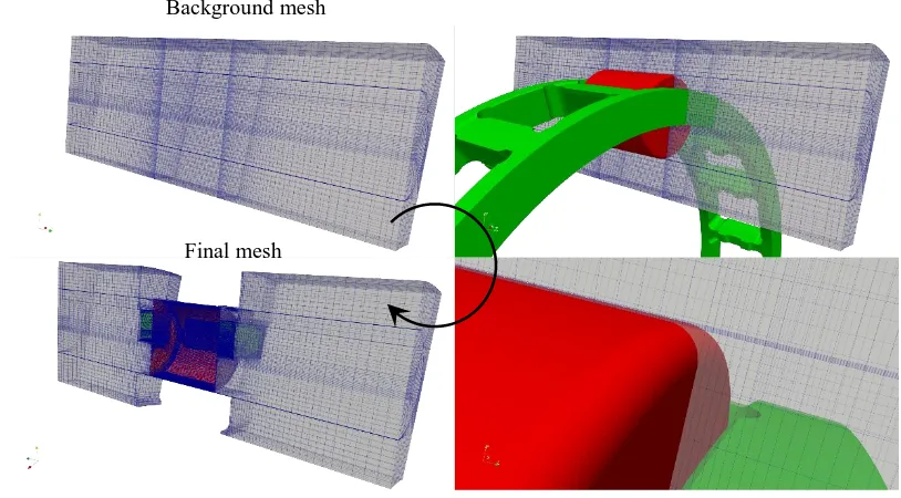
Final mesh
5th mesh
167
Figure 6. Meshing approach for configuration #3: no AMIs are present. Details of the subtraction:
168
background mesh and .stl files on the left; final mesh after the subtraction on the right.
169
This approach is very effective but not as efficient as the analytical generation. The conversion
170
of the background grid into the final mesh takes about 75 s. This is in any case a much better results
171
with respect to a comparable automatic tetrahedralization which took, using a Netgen [18] algorithm,
172
about 900 s.
173
174
Table 3. Parameters of the meshes
175
Mesh #1 #2 #3 #4
points: 1343430 1297328 1035502 17277372 faces: 3832976 3226656 3874220 65442418
cells: 1245328 967904 1442282 24518794
176
Table 3 summarize the properties of the meshes obtained with the different approaches. The
177
number of cells reduces from configuration #1 to #2 due to the presence, in the latter one, of the ribs
178
that limit the volume of the computational domain. Mesh #3 has the highest number of cells because,
179
to accurately follow the rounding radii, the above described mesh splitting step produces a much
180
finer grid near the boundaries. This is confirmed by a higher number of faces of the grid of
181
configuration #3 that, except for the rounding radii, is very similar to configuration #2.
182
2.4.4. Full model
183
To understand the effect of gravity (which relative orientation is a function of the bearing sector
184
position) on the oil flow through and oil distribution in the bearing, , a simulation of the full geometry
185
was also performed. For the rotational speed considered, no significant differences in terms of losses
186
and lubricant distribution are expected with respect to the sectorial model. Nevertheless, to have a
187
complete understanding of the physical phenomena, it is fundamental to investigate also this effect.
188
To build the full grid, a circular pattern of the sectorial mesh #3 was made. The different meshes
189
are conformal and can be easily stitched together. Therefore, the number of cells of the #4 grid results
190
17 (number of rollers) times larger with respect to the mesh #3.
191
193
Figure 6. Mesh #4 (groups with reference to figure 4)
194
2.5. Boundary conditions and mesh motion
195
A 2-phase incompressible, isothermal solver for immiscible fluids was used. It is based on a VOF
196
(volume of fluid) phase-fraction interface capturing approach. In such applications, in fact, the air
197
flows are as important as the lubricant one and a single-phase simplification is not acceptable. A rigid
198
mesh motion without topology changes or adaptive re-meshing was imposed to simulate the motion
199
of the components. The rotational speed of the grid corresponds to the rotational speed of the cage
200
(1904 rpm). This has required the development of two boundary conditions (B.C.) to properly assign
201
the rotational speed to the different components. Since the grid is rotating, the rotational speed of the
202
rings should be defined in the rotating reference frame by adding (inner ring) or subtracting (outer
203
ring) the proper velocities. In the same way, the roto-translation of the rollers is obtained by adding
204
a pure rotation to the motion of the grid. Table 4 summarizes all the B.C..
205
206
Table 4. B.C.
207
Patch U [m/s] / [rpm] p [Pa] [-]
Roller zrel=-14300 p=0 =0
Outer Ring zrel=-1904 p=0 =0
Inner Ring zrel=2596 p=0 =0
Cage rel=0 p=0 =0
Inlet u=0 p=0 =1
Outlet u=0 p=100000 =0
Outlet geometry noSlip p=0 =0
Symmetry symmetry symmetry symmetry
Cyclic cyclic cyclic cyclic
208
Gravity was considered. Simulation were performed limiting the Co number to 1 to ensure
209
numerical stability and good convergence. The solution of the system was performed with a PIMPLE
210
(merged PISO-SIMPLE) algorithm. This conjugates the advantages in terms of computational
211
efficiency of the SIMPLE scheme with the capability of the PISO one to be time-conservative.
212
Mass, momentum and volume fraction conservation equations were defined as follows:
213
𝜕𝜌
𝜕𝑡+ ∇ ∙ (𝜌𝒖) = 0
214
𝜕(𝜌𝒖)
𝜕𝑡 + ∇ ∙ (𝜌𝒖𝒖) = −∇𝑝 + ∇ ∙ [𝜇(∇𝒖 + ∇𝒖
𝑇)] + 𝜌𝒈 + 𝑭
215
𝜕
𝜕𝑡𝛼 +
𝜕
𝜕𝑥𝑖
(𝛼𝑢𝑖) = 0
216
where 𝜌 is the density, 𝒖 is the velocity vector, 𝜇 is the kinematic viscosity of the lubricant, 𝒈
217
is the gravitational acceleration and 𝑭 represents the external forces. 𝛼 is a scalar that represents the
218
of the mixture in each cell of the domain are calculated as an 𝛼-averaged value of the properties of
220
air and lubricant.
221
222
𝜙 = 𝜙𝑙𝑢𝑏∙ 𝛼 + 𝜙𝑎𝑖𝑟∙ (1 − 𝛼)
223
3. Results
224
The main goal of the project was to study the effects of the geometrical simplifications on the
225
lubricant distribution and the power losses. The sectorial simulations were performed on the VSC
226
cluster [19] while the full simulation (#4) on a Deploy Linux LXD [20] Compute Node [21] backed by
227
a Ceph storage cluster [22]. Table 5 summarizes the properties of the computational nodes.
228
229
Table 5. Hardware
230
Name CPU x node Ram x node
VSC 2xAMD Opteron Magny Cours 6132HE (8 Cores, 2.2GHz) 8x4Gb ECC DDR3 LXD 2xINTEL Xeon® E5-2680 (8 Cores, 3.5GHz) 12x32Gb ECC DIMMs
231
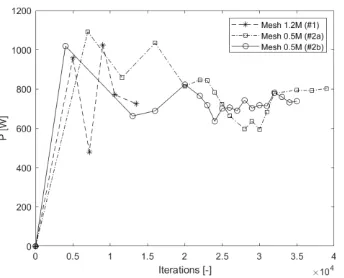
Figure 7 reports the predicted power losses of the different configurations. Despite the different
232
geometries, mostly between #1 and #2 (ribs), the power losses result comparable. However, it is
233
opinion of the authors that these results cannot be generalized to different rotational speeds. The
234
rounding radii seem to not affect significantly the power dissipation. It can be observed that the
235
regime condition (stabilization of the losses) is reached much faster in the simulation #1. The absence
236
of ribs, in fact, promotes an easier lubricant flow in the axial direction.
237
238
Figure 7. Power losses of the bearing.
239
While simplification #1 seems to significantly modify the physical problem producing meaningless
240
results, figure 7 shows the effect of the rounding radii. On the left-hand side #2 is shown. The absence
241
of the rounding radii on the external race causes a stagnation of the lubricant and a higher wetting of
242
the outer radial surface of the cage. This impacts also on the wetting of the radial surface of the roller
243
that results less lubricated in configuration #3.
244
245
Figure 9 highlights the differences induced by the relative position to the roller with respect to
246
the gravitational acceleration. It appears how small differences in terms of oil distribution are present
247
even if the structure of the bearing is axis-symmetric and the mesh is the same for each sector. The
248
250
251
Figure 8. Effect of the rounding radii: wetted surfaces (contour of the volume fraction 0÷1) of cage
252
and roller - models #2 (left) vs #3 (right).
253
254
Figure 9. Effect of the gravitational force: wetted surfaces (contour of the volume fraction 0÷1) of cage
255
and rollers - #4
256
3.1. Computational effort and scalability
257
The 7.3M- and the 1.2M-cells meshes (configuration #1) were used to assess the scalability of the
258
numerical model on the number of processors. For the finer grid, simulations were performed on the
259
VSC cluster using 64, 128 and 256 cores. Figure 10 (left) shows the good scalability of the results. The
260
same was made for the 1.2M mesh. While the scalability seems to be linear up to 64 cores, the time
261
required for the solution does not reduce significantly with 128 cores. With 256 cores, the
262
computational effort even increases. This is due to the times required for the exchange of information
263
between processors that become higher than the solution time itself. The perfect balance was found
264
to be around 20k cells per core.
265
266
Figure 10. Scalability on number of processors (#1 - VSC)
267
5. Conclusions
269
OpenFoam® 4.1 with some specifically developed B.C. seems to be suitable for lubrication
270
simulations. A sector of a Schaeffler NU222-E-XL-M1 bearing was modelled with hexahedral
271
elements taking advantage of different meshing strategies. The studied geometrical simplifications
272
seem to not significantly affect the power losses but unquestionably the lubricant distribution and
273
lubrication of the different components. The presence of the rounding radii on the outer ring
274
promotes the lubricant circulation reducing its stagnation between cage and rings. The components
275
result less wetted.
276
The gravity seems to slightly affect the wetting of the rollers depending on their position along
277
the circumference of the bearing.
278
279
The proposed meshing approaches enable different levels of geometrical complexity. The
280
capability to create a 3D grid starting from a simple extrusion allows a much better control of the
281
mesh quality that directly affects the convergence of the solution and, therefore, the computational
282
effort required.
283
284
Scalability tests have shown, for 2 different grids, that an averaged number of cells per core of
285
about 20k is the best balance between computational resources and computational effort (on the
286
present hardware).
287
288
Funding: This research was funded by Schaeffler Technologies AG & Co. KG, grant number TN2369-C and
289
TN2371-C.
290
Acknowledgments: The authors would thank Cristiano Cumer for the support with the LXD cluster.
291
Conflicts of Interest: authors declare no conflict of interest
292
References
293
[1] Z. Ji, M. Stanic, E. A. Hartono, and V. Chernoray, “Numerical simulations of oil flow inside a gearbox
294
by Smoothed Particle Hydrodynamics (SPH) method,” Tribol. Int., vol. 127, pp. 47–58, 2018.
295
[2] F. Concli and C. Gorla, “Windage, churning and pocketing power losses of gears: different modeling
296
approaches for different goals,” Forsch. im Ingenieurwesen/Engineering Res., vol. 80, no. 3–4, 2016.
297
[3] P. H. L. Groenenboom, M. Z. Mettichi, and Y. Gargouri, “Simulating Oil Flow for Gearbox Lubrication
298
using Smoothed Particle Hydrodynamics,” Proc. Int. Conf. Gears 2015, 2015.
299
[4] F. Concli and C. Gorla, “CFD simulation of power losses and lubricant flows in gearboxes,” in American
300
Gear Manufacturers Association Fall Technical Meeting 2017, 2017, vol. 2017-Janua.
301
[5] Ted Ørjan Kjellevik Gundersen, “Modelling of Rotating Turbulent Flows,” NTNU, 2011.
302
[6] F. Concli, C. Gorla, A. D. Torre, and G. Montenegro, “Windage power losses of ordinary gears: Different
303
CFD approaches aimed to the reduction of the computational effort,” Lubricants, vol. 2, no. 4, pp. 162–
304
176, 2014.
305
[7] M. Wang, X. Xu, X. Ren, C. Li, J. Chen, and X. Yang, “Mesh partitioning using matrix value
306
approximations for parallel computational fluid dynamics simulations,” Adv. Mech. Eng., vol. 9, no. 11,
307
[8] F. Concli and C. Gorla, “Numerical modeling of the churning power losses in planetary gearboxes: An
309
innovative partitioning-based meshing methodology for the application of a computational effort
310
reduction strategy to complex gearbox configurations,” Lubr. Sci., 2017.
311
[9] C. J. Hwang and S. J. Wu, “Global and local remeshing algorithms for compressible flows,” J. Comput.
312
Phys., vol. 102, no. 1, pp. 98–113, 1992.
313
[10] J. Zheng, J. Chen, Y. Zheng, Y. Yao, S. Li, and Z. Xiao, “An improved local remeshing algorithm for
314
moving boundary problems,” Eng. Appl. Comput. Fluid Mech., vol. 10, no. 1, pp. 403–426, 2016.
315
[11] F. Concli, A. Della Torre, C. Gorla, and G. Montenegro, “A New Integrated Approach for the Prediction
316
of the Load Independent Power Losses of Gears: Development of a Mesh-Handling Algorithm to Reduce
317
the CFD Simulation Time,” Adv. Tribol., vol. 2016, 2016.
318
[12] F. Concli and C. Gorla, “Numerical modeling of the power losses in geared transmissions: Windage,
319
churning and cavitation simulations with a new integrated approach that drastically reduces the
320
computational effort,” Tribol. Int., vol. 103, 2016.
321
[13] J. M. Rubio, “Multidimensional simulations of external gear pumps,” Politecnico di Milano, 2017.
322
[14] F. Concli, “Pressure distribution in small hydrodynamic journal bearings considering cavitation: a
323
numerical approach based on the open-source CFD code OpenFOAM®,” Lubr. Sci., vol. 28, no. 6, 2016.
324
[15] F. Concli and C. Gorla, “Analysis of the oil squeezing power losses of a spur gear pair by mean of CFD
325
simulations,” in ASME 2012 11th Biennial Conference on Engineering Systems Design and Analysis, ESDA
326
2012, 2012, vol. 2.
327
[16] F. Concli and C. Gorla, “Oil squeezing power losses in gears: A CFD analysis,” in WIT Transactions on
328
Engineering Sciences, 2012, vol. 74.
329
[17] “OpenFOAM User Guide.” .
330
[18] “www.hpfem.jku.at/netgen/.” .
331
[19] “http://vsc.ac.at/.” .
332
[20] “https://linuxcontainers.org/.” .
333
[21]
“https://www.cisco.com/c/dam/en/us/products/collateral/servers-unified-computing/ucs-b-series-334
blade-servers/B200M3_SpecSheet.pdf.” .
335
[22] “https://ceph.com.” .