VARIATIONAL ALGORITHMS FOR
APPROXIMATE BAYESIAN INFERENCE
b y
Matthew J. Beal
M.A., M^Sei., Physics, University of Cambridge, UK (1998)
UCL
The Gatsby Computational Neuroscience Unit
University College London
17 Queen Square London WCIN 3AR
A Thesis submitted for the degree of
Doctor of Philosophy of the University of London
ProQuest Number: 10016139
All rights reserved
INFORMATION TO ALL USERS
The quality of this reproduction is dependent upon the quality of the copy submitted.
In the unlikely event that the author did not send a complete manuscript and there are missing pages, these will be noted. Also, if material had to be removed,
a note will indicate the deletion.
uest.
ProQuest 10016139
Published by ProQuest LLC(2016). Copyright of the Dissertation is held by the Author.
All rights reserved.
This work is protected against unauthorized copying under Title 17, United States Code. Microform Edition © ProQuest LLC.
ProQuest LLC
789 East Eisenhower Parkway P.O. Box 1346
Abstract
The Bayesian framework for machine learning allows for the incorporation of prior knowledge in a coherent way, avoids overfitting problems, and provides a principled basis for selecting between alternative models. Unfortunately the computations required are usually intractable. This thesis presents a unified variational Bayesian (VB) framework which approximates these computations in models with latent variables using a lower bound on the marginal likelihood.
Chapter 1 presents background material on Bayesian inference, graphical models, and propaga tion algorithms. Chapter 2 forms the theoretical core of the thesis, generalising the expectation- maximisation (EM) algorithm for learning maximum likelihood parameters to the VB EM al gorithm which integrates over model parameters. The algorithm is then specialised to the large family of conjugate-exponential (CE) graphical models, and several theorems are presented to pave the road for automated VB derivation procedures in both directed and undirected graphs (Bayesian and Markov networks, respectively).
Acknowledgements
I am very grateful to my advisor Zoubin Ghahramani for his guidance in this work, bringing energy and thoughtful insight into every one of our discussions. I would also like to thank other senior Gatsby Unit members including Hagai Attias, Phil Dawid, Peter Dayan, Geoff Hinton, Carl Rasmussen and Sam Roweis, for numerous discussions and inspirational comments.
My research has been punctuated by two internships at Microsoft Research in Cambridge and in Redmond. Whilst this thesis does not contain research carried out in these labs, I would like to thank colleagues there for interesting and often seductive discussion, including Christopher Bishop, Andrew Blake, David Heckerman, Nebojsa Jojic and Neil Lawrence.
Amongst many others I would like to thank especially the following people for their support and useful comments: Andrew Brown, Nando de Freitas, Oliver Downs, Alex Gray, Yoel Haitovsky, Sham Kakade, Alex Korenberg, David MacKay, James Miskin, Quaid Morris, Iain Murray, Radford Neal, Simon Osindero, Lawrence Saul, Matthias Seeger, Amos Storkey, Yee-Whye Teh, Eric Tuttle, Naonori Ueda, John Winn, Chris Williams, and Angela Yu.
I should thank my friends, in particular Paola Atkinson, Tania Lillywhite, Amanda Parmar, James Tinworth and Mark West for providing me with various combinations of shelter, com panionship and retreat during my time in London. Last, but by no means least I would like to thank my family for their love and nurture in all my years, and especially my dear fiancée Cassandre Creswell for her love, encouragement and endless patience with me.
Contents
Abstract 2
Acknowledgements 3
Contents 4
List of figures 8
List of tables 11
List of algorithms 12
1 Introduction 13
1.1 Probabilistic inference ... 16
1.1.1 Probabilistic graphical models: directed and undirected networks . . . 17
1.1.2 Propagation algorithm s... 19
1.2 Bayesian model selection ... 24
1.2.1 Marginal likelihood and Occam’s r a z o r ... 25
1.2.2 Choice of priors... 27
1.3 Practical Bayesian a p p ro a c h e s... 32
1.3.1 Maximum a posteriori (MAP) parameter e s tim a te s ... 33
1.3.2 Laplace’s m etho d... 34
1.3.3 Identifiability: aliasing and d e g e n e ra c y ... 35
1.3.4 BIC and MDL ... 36
1.3.5 Cheeseman & Stutz’s m e t h o d ... 37
1.3.6 Monte Carlo m ethods... 38
1.4 Summary of the remaining c h a p t e r s ... 42
2 Variational Bayesian Theory 44 2.1 Introduction... 44
2.2 Variational methods for ML / MAP le arn in g ... 46
2.2.1 The scenario for parameter le a rn in g ... 46
Contents________________________________________________ Contents
2.2.3 EM with constrained (approximate) o p tim isatio n ... 49
2.3 Variational methods for Bayesian le arn in g ... 53
2.3.1 Deriving the learning r u le s ... 53
2.3.2 D is c u s sio n ... 58
2.4 Conjugate-Exponential m o d e ls ... 64
2.4.1 D efinition... 64
2.4.2 Variational Bayesian EM for CE m odels... 66
2.4.3 Implications ... 69
2.5 Directed and undirected g ra p h s... 73
2.5.1 Implications for directed netw orks... 73
2.5.2 Implications for undirected networks ... 74
2.6 Comparisons of VB to other c r it e r ia ... 75
2.6.1 BIC is recovered from VB in the limit of large d a t a ... 75
2.6.2 Comparison to Cheeseman-Stutz (CS) approximation... 76
2.7 S u m m a ry ... 80
3 Variational Bayesian Hidden Markov Models 82 3.1 Introduction... 82
3.2 Inference and learning for maximum likelihood H M M s ... 83
3.3 Bayesian HMMs ... 88
3.4 Variational Bayesian form ulation... 91
3.4.1 Derivation of the VBEM optimisation p ro c e d u r e ... 92
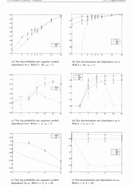
3.4.2 Predictive probability of the VB m o d e l ... 97
3.5 Experim ents... 98
3.5.1 Synthetic: discovering model structure ... 98
3.5.2 Forwards-backwards English discrimination... 99
3.6 Discussion... 104
4 Variational Bayesian Mixtures of Factor Analysers 106 4.1 Introduction... 106
4.1.1 Dimensionality reduction using factor a n a l y s i s ... 107
4.1.2 Mixture models for manifold le a rn in g ... 109
4.2 Bayesian Mixture of Factor A n a ly s e rs ... 110
4.2.1 Parameter priors for M F A ...I l l 4.2.2 Inferring dimensionality using A R D ... 114
4.2.3 Variational Bayesian derivation ...115
4.2.4 Optimising the lower b o u n d ... 119
4.2.5 Optimising the hyperparam eters... 122
4.3 Model exploration: birth and d e a th ... 124
4.3.1 Heuristics for component d e a t h ... 126
Contents____________________________________________________________ Contents
4.3.3 Heuristics for the optimisation endgam e...130
4.4 Handling the predictive d en sity... 130
4.5 Synthetic experiments... 132
4.5.1 Determining the number of com ponents...133
4.5.2 Embedded Gaussian c lu ste rs... 133
4.5.3 Spiral d a ta s e t... 135
4.6 Digit experim ents...138
4.6.1 Fully-unsupervised le a r n in g ... 138
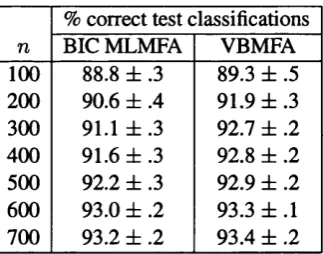
4.6.2 Classification performance of BIC and VB m o d e ls ...141
4.7 Combining VB approximations with Monte C a r lo ... 144
4.7.1 Importance sampling with the variational approxim ation... 144
4.7.2 Example: Tightness of the lower bound for M FA s...148
4.7.3 Extending simple importance s a m p lin g ...151
4.8 S u m m a ry ... 157
5 Variational Bayesian Linear Dynamical Systems 159 5.1 Introduction... 159
5.2 The Linear Dynamical System model ... 160
5.2.1 Variables and to p o lo g y ... 160
5.2.2 Specification of parameter and hidden state p rio rs...163
5.3 The variational tre a tm e n t... 168
5.3.1 VBM step: Parameter distributions...170
5.3.2 VBE step: The Variational Kalman S m o o th er... 173
5.3.3 Filter (forward recursion)...174
5.3.4 Backward recursion: sequential and p arallel... 177
5.3.5 Computing the single and joint m a rg in a ls ... 181
5.3.6 Hyperparameter learn in g ...184
5.3.7 Calculation of ... 185
5.3.8 Modifications when learning from multiple sequences ... 186
5.3.9 Modifications for a fully hierarchical m o d e l... 189
5.4 Synthetic E x p e rim e n ts ... 189
5.4.1 Hidden state space dimensionality determination (no in p u ts ) ...189
5.4.2 Hidden state space dimensionality determination (input-driven) . . . . 191
5.5 Elucidating gene expression mechanisms ... 195
5.5.1 Generalisation e r r o r s ... 198
5.5.2 Recovering gene-gene interactions...200
5.6 Possible extensions and future research ...201
5.7 S u m m a ry ... 204
6 Learning the structure of discrete-variable graphical models with hidden vari
Contents Contents
6.1 Introduction... 206
6.2 Calculating marginal likelihoods of D A G s ... 207
6.3 Estimating the marginal likelih oo d ...210
6.3.1 ML and MAP parameter e s tim a tio n ...210
6.3.2 B I C ... 212
6.3.3 Cheesem an-Stutz... 213
6.3.4 The VB lower b o u n d ... 215
6.3.5 Annealed Importance Sampling (A I S )...218
6.3.6 Upper bounds on the marginal lik e lih o o d ...222
6.4 Experim ents... 223
6.4.1 Comparison of scores to A I S ... 226
6.4.2 Performance averaged over the parameter p r i o r ... 232
6.5 Open questions and d ir e c tio n s ... 236
6.5.1 AIS analysis, limitations, and extensions ...236
6.5.2 Estimating dimensionalities of the incomplete and complete-data models 245 6 .6 S u m m a ry ...247
7 Conclusion 250 7.1 Discussion...250
7.2 Summary of contributions ... 254
Appendix A Conjugate Exponential family examples 259 Appendix B Useful results from matrix theory 262 B.l Schur complements and inverting partitioned m atrices...262
B.2 The matrix inversion l e m m a ... 263
Appendix C Miscellaneous results 265 C.l Computing the digamma function ...265
C.2 Multivariate gamma hyperparameter optim isation...266
C.3 Marginal KL divergence of gamma-Gaussian v a ria b le s ...267
List of figures
1.1 The elimination algorithm on a simple Markov netw ork... 20
1.2 Forming the junction tree for a simple Markov n e tw o rk ... 22
1.3 The marginal likelihood embodies Occam’s r a z o r ... 27
2.1 Variational interpretation of EM for ML l e a r n in g ... 50
2.2 Variational interpretation of constrained EM for ML le a rn in g ... 51
2.3 Variational Bayesian E M ... 56
2.4 Hidden-variable / parameter factorisation steps ... 59
2.5 Hyperparameter learning for VB E M ... 62
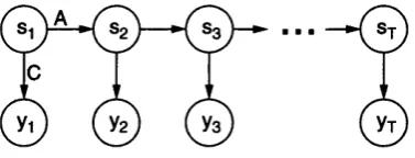
3.1 Graphical model representation of a hidden Markov m o d e l ... 83
3.2 Evolution of the likelihood for ML hidden Markov models, and the subsequent VB lower bound... 100
3.3 Results of ML and VB HMM models trained on synthetic sequences... 101
3.4 Test data log predictive probabilities and discrimination rates for ML, MAP, and VB H M M s ... 103
4.1 ML Mixtures of Factor Analysers ... 110
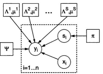
4.2 Bayesian Mixtures of Factor Analysers... 114
4.3 Determination of number of components in synthetic d a ta ... 134
4.4 Factor loading matrices for dimensionality determ ination... 135
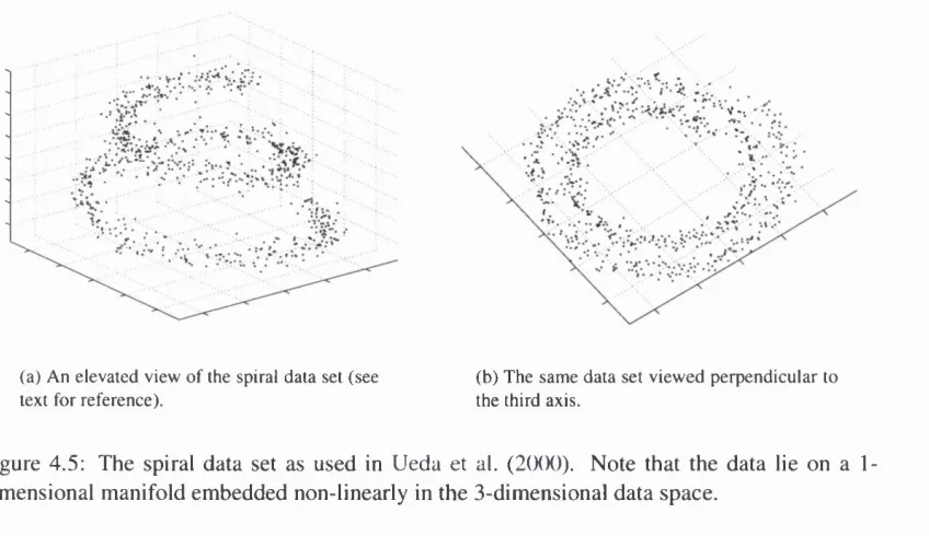
4.5 The Spiral data set of Ueda et. a l ... 136
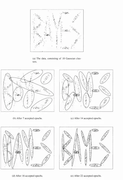
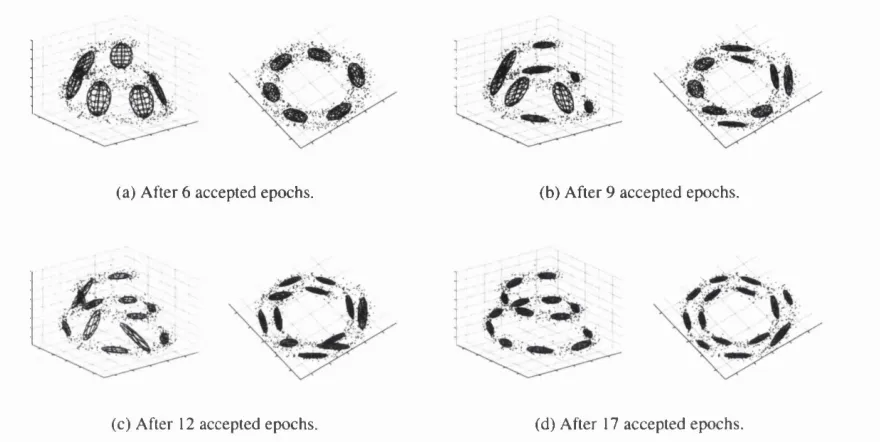
4.6 Birth and death processes with VBMFA on the Spiral data s e t ... 137
4.7 Evolution of the lower bound T for the Spiral data s e t ... 137
4.8 Training examples of digits from the C E D A R database... 138
4.9 A typical model of the digits learnt by V B M F A ... 139
4.10 Confusion tables for the training and test digit classifications... 140
4.11 Distribution of components to digits in BIC and VB m odels... 143
4.12 Logarithm of the marginal likelihood estimate and the VB lower bound during learning of the digits { 0 ,1 ,2 } ... 150
List o f figures List o f figures
4.14 Importance sampling estimates of marginal likelihoods for learnt models of
data of differently spaced clusters ... 156
5.1 Graphical model representation of a state-space model ... 161
5.2 Graphical model for a state-space model with inputs... 162
5.3 Graphical model representation of a Bayesian state-space m o d e l ... 164
5.4 Recovered LDS models for increasing data s i z e ... 190
5.5 Hyperparameter trajectories showing extinction of state-space dimensions . . . 191
5.6 Data for the input-driven LDS synthetic experim ent... 193
5.7 Evolution of the lower bound and its g r a d ie n t... 194
5.8 Evolution of precision hyperparameters, recovering true model structure . . . . 196
5.9 Gene expression data for input-driven experiments on real d a t a ... 197
5.10 Graphical model of an LDS with feedback of observations into i n p u t s 199 5.11 Reconstruction errors of LDS models trained using MAP and VB algorithms as a function of state-space dim ensionality...20 0 5.12 Gene-gene interaction matrices learnt by MAP and VB algorithms, showing significant e n tr ie s ...2 0 2 5.13 Illustration of the gene-gene interactions learnt by the feedback model on ex pression data ... 203
6.1 The chosen structure for generating data for the e x p erim en ts... 225
6.2 Illustration of the trends in marginal likelihood estimates as reported by MAP, BIC, BICp, CS, VB and AIS methods, as a function of data set size and number of p a ra m e te rs ... 228
6.3 Graph of rankings given to the true structure by BIC, BICp, CS, VB and AIS m e th o d s... 230
6.4 Differences in marginal likelihood estimate of the top-ranked and true struc tures, by BIC, BICp, CS, VB and AIS ... 232
6.5 The median ranking given to the true structure over repeated settings of its parameters drawn from the prior, by BIC, BICp, CS and VB methods ...233
6 .6 Median score difference between the true and top-ranked structures, under BIC, BICp, CS and VB methods... 234
6.7 The best ranking given to the true structure by BIC, BICp, CS and VB methods 235 6.8 The smallest score difference between true and top-ranked structures, by BIC, BICp, CS and VB m e th o d s ... 236
6.9 Overall success rates of BIC, BICp, CS and VB scores, in terms of ranking the true structure t o p ...237
List o f figures List o f figures
6.11 Acceptance rates of the Metropolis-Hastings proposals as a function of size of data set ... 240 6.12 Acceptance rates of the Metropolis-Hastings sampler in each of four quarters
List of tables
2.1 Comparison of EM for ML/MAP estimation against VB EM with CE models . 70
4.1 Simultaneous determination of number of components and their dimensionalities 135 4.2 Test classification performance of BIC and VB m o d e ls ... 142 4.3 Specifications of six importance sampling distribu tio ns... 155
6.1 Rankings of the true structure amongst the alternative candidates, by MAP, BIC, BICp, VB and AIS estimates, both corrected and uncorrected for posterior a l ia s in g ... 230 6.2 Comparison of performance of VB to BIC, BICp and CS methods, as measured
by the ranking given to the true m o d e l... 233 6.3 Improving the AIS estimate by pooling the results of several separate sampling
r u n s ...241 6.4 Rate of AIS violations of the VB lower bound, alongside Metropolis-Hastings
rejection r a t e s ... 241 6.5 Number of times the true structure is given the highest ranking by the BIC,
List of Algorithms
5.1 Forward recursion for variational Bayesian state-space m o d e ls ...178
5.2 Backward parallel recursion for variational Bayesian state-space models . . . . 181
5.3 Pseudocode for variational Bayesian state-space m odels... 187 6.1 AIS algorithm for computing all ratios to estimate the marginal likelihood . . . 221 6.2 Algorithm to estimate the complete- and incomplete-data dimensionalities of a
Chapter 1
Introduction
Our everyday experiences can be summarised as a series of decisions to take actions which manipulate our environment in some way or other. We base our decisions on the results of predictions or inferences of quantities that have some bearing on our quality of life, and we come to arrive at these inferences based on models of what we expect to observe. Models are designed to capture salient trends or regularities in the observed data with a view to predicting future events. Sometimes the models can be constructed with existing expertise, but for the majority of real applications the data are far too complex or the underlying processes not nearly well enough understood for the modeller to design a perfectly accurate model. If this is the case, we can hope only to design models that are simplifying approximations of the true processes that generated the data.
For example, the data might be a time series of the price of stock recorded every day for the last six months, and we would like to know whether to buy or sell stock today. This decision, and its particulars, depend on what the price of the stock is likely to be a week from now. There are obviously a very large number of factors that influence the price and these do so to varying degrees and in convoluted and complex ways. Even in the unlikely scenario that we knew exactly how all these factors affected the price, we would still have to gather every piece of data for each one and process it all in a short enough time to decide our course of action. Another example is trying to predict the best location to drill for oil, knowing the positions of existing drill sites in the region and their yields. Since we are unable to probe deep beneath the Earth’s surface, we need to rely on a model of the geological processes that gave rise to the yields in those sites for which we have data, in order to be able to predict the best location.
The machine teaming approach to modelling data constructs models by beginning with a flexi
Introduction
that the particular setting of the best-fit parameters provides us with some understanding of the underlying processes. The procedure of fitting model parameters to observed data is termed
learning a model.
Since our models are simplifications of reality there will inevitably be aspects of the data which cannot be modelled exactly, and these are considered noise. Unfortunately it is often difficult to know which aspects of the data are relevant for our inference or prediction tasks, and which aspects should be regarded as noise. With a sufficiently complex model, parameters can be found to fit the observed data exactly, but any predictions using this best-fit model will be sub- optimal as it has erroneously fitted the noise instead of the trends. Conversely, too simple a model will fail to capture the underlying regularities in the data and so will also produce sub- optimal inferences and predictions. This trade-off between the complexity of the model and its generalisation performance is well studied, and we return to it in section 1.2.
The above ideas can be formalised using the concept of probability and the rules of Bayesian inference. Let us denote the data set by y, which may be made up of several variables indexed by j: y = { y i , . . . , y j , . . . , yjr}. For example, y could be the data from an oil well for which the variables might be measurements of the type of oil found, the geographical location of the well, its average monthly yield, its operational age, and a host of other measurable quantities regarding its local geological characteristics. Generally each variable can be real-valued or discrete. Machine learning approaches define a generative model of the data through a set of parameters d = { ^ i , . . . , 0 ^} which define a probability distribution over data, p (y 10). One approach to learning the model then involves finding the parameters 6* such that
0* = arg max p(y I 0) . (1.1)
9
This process is often called maximum likelihood learning as the parameters 0* are set to max imise the likelihood of 0, which is probability of the observed data under the model. The generative model may also include latent or hidden variables, which are unobserved yet inter act through the parameters to generate the data. We denote the hidden variables by x, and the probability of the data can then be written by summing over the possible settings of the hidden states:
p i y \ ^ ) = ] ^ p ( x |^ ) p ( y | x , ^ ) , ( L2)
X
Introduction
For a particular parameter setting, it is possible to infer the states of the hidden variables of the model, having observed data, using Bayes’ rule:
This quantity is known as the posterior distribution over the hidden variables. In the oil well example we might have a hidden variable for the amount of oil remaining in the reserve, and this can be inferred based on observed measurements such as the operational age, monthly yield and geological characteristics, through the generative model with parameters 0. The term p ( x 10)
is a prior probability of the hidden variables, which could be set by the modeller to reflect the distribution of amounts of oil in wells that he or she would expect. Note that the probability of the data in (1.2) appears in the denominator of (1.3). Since the hidden variables are by definition unknown, finding 0* becomes more difficult, and the model is learnt by alternating between estimating the posterior distribution over hidden variables for a particular setting of the parameters and then re-estimating the best-fit parameters given that distribution over the hidden variables. This procedure is the well-known expectation-maximisation (EM) algorithm and is discussed in more detail in section 2.2.
Given that the parameters themselves are unknown quantities we can treat them as random variables. This is the Bayesian approach to uncertainty, which treats all uncertain quantities as random variables and uses the laws of probability to manipulate those uncertain quantities. The proper Bayesian approach attempts to integrate over the possible settings of all uncertain quantities rather than optimise them as in (1.1). The quantity that results from integrating out both the hidden variables and the parameters is termed the marginal likelihood:
P{y) = [ d0 p { 0 ) ' ^ p { x I 0)p{y I X, 0) , (1.4)
d X
In troduction 1.1. Probabilistic inference
Unfortunately the marginal likelihood, p{y), is an intractable quantity to compute for almost all models of interest (we will discuss why this is so in section 1.2.1, and see several examples in the course of this thesis). Traditionally, the marginal likelihood has been approximated either using analytical methods, for example the Laplace approximation, or via sampling-based approaches such as Markov chain Monte Carlo. These methods are reviewed in section 1.3. This thesis is devoted to one particular method of approximation, variational Bayes, sometimes referred to as
ensemble learning. The variational Bayesian method constructs a lower bound on the marginal
likelihood, and attempts to optimise this bound using an iterative scheme that has intriguing similarities to the standard expectation-maximisation algorithm. There are other variational methods, for example those based on Bethe and Kikuchi free energies, which for the most part are approximations rather than bounds; these are briefly discussed in the final chapter.
Throughout this thesis we assume that the reader is familiar with the basic concepts of probabil ity and integral and differential calculus. Included in the appendix are reference tables for some of the more commonly used probability distributions.
The rest of this chapter reviews some key methods relevant to Bayesian model inference and learning. Section 1.1 reviews the use of graphical models as a tool for visualising the prob abilistic relationships between the variables in a model and explains how efficient algorithms for computing the posterior distributions of hidden variables as in (1.3) can be designed which exploit independence relationships amongst the variables. In section 1.2, we address the issue of model selection in a Bayesian framework, and explain why the marginal likelihood is the key quantity for this task, and how it is intractable to compute. Since all Bayesian reasoning needs to begin with some prior beliefs, we examine different schools of thought for expressing these priors in section 1.2.2, including conjugate, reference, and hierarchical priors. In section 1.3 we review several practical methods for approximating the marginal likelihood, which we shall be comparing to variational Bayes in the following chapters. Finally, section 1.4 briefly summarises the remaining chapters of this thesis.
1.1 Probabilistic inference
Bayesian probability theory provides a language for representing beliefs and a calculus for ma nipulating these beliefs in a coherent manner. It is an extension of the formal theory of logic which is based on axioms that involve propositions that are true or false. The rules of proba bility theory involve propositions which have plausibilities of being true or false, and can be arrived at on the basis of just three desiderata: (1) degrees of plausibility should be represented
by real numbers; (2) plausibilities should have qualitative correspondence with common sense;
Introduction 1.1. Probabilisticinference
(Cox, 1946), Cox showed that plausibilities can be measured on any scale and it is possible to transform them onto the canonical scale of probabilities that sum to one. For good introductions to probability theory the reader is referred to Pearl (1988) and Jaynes (2(X)3).
Statistical modelling problems often involve large numbers of interacting random variables and it is often convenient to express the dependencies between these variables graphically. In par ticular such graphical models are an intuitive tool for visualising conditional independency re lationships between variables. A variable a is said to be conditionally independent of h, given c if and only if p{a, b | c) can be written p{a \ c)p(h | c). By exploiting conditional independence relationships, graphical models provide a backbone upon which it has been possible to derive efficient message-propagating algorithms for conditioning and marginalising variables in the model given observation data (Pearl, 1988; Lauritzen and Spiegelhalter, 1988; Jensen, 1996; Heckerman, 1996; Cowell et al., 1999; Jordan, 1999). Many standard statistical models, espe cially Bayesian models with hierarchical priors (see section 1.2.2), can be expressed naturally using probabilistic graphical models. This representation can be helpful in developing both sam pling methods (section 1.3.6) and exact inference methods such as the junction tree algorithm (section 1.1.2) for these models. All of the models used in this thesis have very simple graphi cal model descriptions, and the theoretical results derived in chapter 2 for variational Bayesian approximate inference are phrased to be readily applicable to general graphical models.
1.1.1 Probabilistic graphical models: directed and undirected networks
A graphical model expresses a family of probability distributions on sets of variables in a model. Here and for the rest of the thesis we use the variable z to denote all the variables in the model, be they observed or unobserved (hidden). To differentiate between observed and unobserved variables we partition z into z = {x, y } where x and y are the sets of unobserved and observed variables, respectively. Alternatively, the variables are indexed by the subscript j , with j £ 7i
the set of indices for unobserved (hidden) variables and j G V the set of indices for observed variables. We will later introduce a further subscript, i, which will denote which data point out of a data set of size n is being referred to, but for the purposes of the present exposition we consider just a single data point and omit this further subscript.
Each arc between two nodes in the graphical model represents a probabilistic connection be tween two variables. We use the terms ‘node’ and ‘variable’ interchangeably. Depending on the pattern of arcs in the graph and their type, different independence relations can be represented between variables. The pattern of arcs is commonly referred to as the structure of the model.
The arcs between variables can be all directed or all undirected. There is a class of graphs in
which some arcs are directed and some are undirected, commonly called chain graphs, but these
Introduction 1.1. Probabilisticinference
random fields, express the probability distribution over variables as a product over clique poten
tials’.
1 J
P(z) =
2
n
’
(1-5)
;= i
where z is the set of variables in the model, are cliques of the graph, and
are a set of clique potential functions each of which returns a non-negative real value for every possible configuration of settings of the variables in the clique. Each clique is defined to be a fully connected subgraph (that is to say each clique Cj selects a subset of the variables in z), and is usually maximal in the sense that there are no other variables whose inclusion preserves its fully connected property. The cliques can be overlapping, and between them cover all variables such that {C'i(z) U • • • U (7j(z)} = z. Here we have written a normahsation constant, Z ,
into the expression (1.5) to ensure that the total probability of all possible configurations sums to one. Alternatively, this normalisation can be absorbed into the definition of one or more of the potential functions. Markov networks can express a very simple form of independence relationship: two sets of nodes A and B are conditionally independent from each other given a third set of nodes C, if all paths connecting any node in A to any node in B via a sequence of arcs are separated by any node (or group of nodes) in C. Then C is said to separate A from B.
The Markov blanket for the node (or set of nodes) A is defined as the smallest set of nodes C,
such that A is conditionally independent of all other variables not in C, given C.
Directed graphical models, also called Directed Acyclic Graphs (DAGs), or Bayesian networks,
express the probability distribution over J variables, z = as a product of conditional
probability distributions on each variable:
J
p(z) = ’ (1-6)
j= i
where Zpa(j) is the set of variables that are parents of the node j in the graph. A node a is said to be a parent of a node b if there is a directed arc from a to b, and in which case b is said to be a child of a. In necessarily recursive definitions: the descendents of a node are defined to include its children and its childrens’ descendents; and the ancestors of a node are its parents and those parents’ ancestors. Note that there is no need for a normalisation constant in (1.6) because by the definition of the conditional probabilities it is equal to one. A directed path
Introduction 1.1. Probabilisticinference
More generally, we have the following representation of independence in Bayesian networks: two sets of nodes A and B are conditionally independent given the set of nodes C if they are
d-separated by C (here the d- prefix stands for directed). The nodes A and B are d-separated by
C if, along every undirected path from A to B, there exists a node d which satisfies either of the following conditions: either (i) d has converging arrows (i.e. d is the child of the previous node and the parent of the following node in the path) and neither d nor its descendents are in C; or (ii) d does not have converging arrows and is in C. From the above definition of the Markov blanket, we find that for Bayesian networks the minimal Markov blanket for a node is given by the union of its parents, its children, and the parents of its children. A more simple rule for d-separation can be obtained using the idea of the ‘Bayes ball’ (Shachter, 1998). Two sets of nodes A and B are conditionally dependent given C if there exists a path by which the Bayes ball can reach a node in B from a node in A (or vice-versa), where the ball can move according to the following rules: it can pass through a node in the conditioning set C provided the entry and exit arcs are a pair of arrows converging on that node; similarly, it can only pass through every node in the remainder of the graph provided it does so on non-converging arrows. If there exist no such linking paths, then the sets of nodes A and B are conditionally independent given C.
Undirected models tend to be used in the physics and vision communities, where the systems under study can often be simply expressed in terms of many localised potential functions. The nature of the interactions often lack causal or direct probabilistic interpretations, and instead express degrees of agreement, compatibility, constraint or frustration between nodes. In the artificial intelligence and statistics communities directed graphs are more popular as they can more easily express underlying causal generative processes that give rise to our observations. For more detailed examinations of directed and undirected graphs see Pearl (1988).
1.1.2 Propagation algorithms
The conditional independence relationships discussed in the previous subsection can be ex ploited to design efficient message-passing algorithms for obtaining the posterior distributions over hidden variables given the observations of some other variables, which is called inference.
In this section we briefly present an inference algorithm for Markov networks, called the junc
tion tree algorithm. We will explain at the end of this subsection why it suffices to present the
inference algorithm for the undirected network case, since the inference algorithm for a directed network is just a special case.
Introduction 1.1. Probabilistic inference
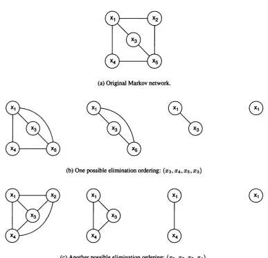
(a) Original M arkov network.
(b) One possible elimination ordering: ( x 2 ,2:4, x s , X3)
©
(c) A nother possible elimination ordering: ( x s , x z , X3, X4 ).
0
Figure 1.1: (a) The original Markov network; (b) The sequence of intermediate graphs resulting from eliminating (integrating out) nodes to obtain the marginal on x i — see equations (1.9- 1.14); (c) Another sequence of graphs resulting from a different elimination ordering, which results in a suboptimal inference algorithm.
practice in these cases is to utilise expectation-maximisation (EM) algorithms, which in their E step require the computation of at least certain properties of the posterior distribution over the hidden variables.
We illustrate the basics of inference using a simple example adapted from Jordan and Weiss (2002). Figure 1.1(a) shows a Markov network for five variables x = { x i , . . . ,0:5}, each of which is discrete and takes on k possible states. Using the Markov network factorisation given by (1.5), the probability distribution over the variables can be written as a product of potentials defined over five cliques:
Introduction 1.1. Probabilisticinference
where we have included a normalisation constant Z to allow for arbitrary clique potentials. Note that in this graph 1.1 (a) the maximal cliques are all pairs of nodes connected by an arc, and therefore the potential functions are defined over these same pairs of nodes. Suppose we wanted to obtain the marginal distribution p{xi), given by
P { x i ) = ^ ' ^ ' ^ ' ^ ' ^ ^ p { X l , X 2 ) ^ p { X l , X 3 ) ' ^ p { x u X 4 ) ' ^ J J { x 2 , X 5 ) ^ p { x 3 , X 5 ) ' ^ p { x 4 , X 5 )
.
X2 X 3 X 4 X 5
(1.8)
At first glance this requires computations, since there are 0 summands to be computed for
each of the k settings of the variable xi . However this complexity can be reduced by exploiting the conditional independence structure in the graph. For example, we can rewrite (1.8) as
P M = V’(a^l, a^s)V'(x3, X 5 ) ' l p { x i , X 4 ) ' l p { x 4 , X ^ ) ' l l ) { x i , X 2 ) i ) { x 2 , X5) (1.9)
X 2 X3 X4 X5
= y Y l ^ ( ^ 1 ’ ^ 3 ) ^ X5) ^ ( z i , Z 4 ) ^ ( Z 4 , Z 5 ) Y 2
Z
X3 X5 X4 X2
(1.10)
= ^ ^ Z 3 ) ^ ^ ( Z 3 , Z 5 ) ^ ^ ( T i , Z 4 )V '(a:4 , 375)7722(3:1, Z 5 ) ( 1 . 1 1 )
Z
X3 X5 X4
= ^ X l ^ ^ ^ i ’^3)X ]^(^3,iC5)m 4(xi,a:5)m 2(a;i,a:5) (1.12)
X3 X5
= ^ ^ ^ ( a ; i , 0 : 3 ) 7 7 1 5 ( 2 : 1 , X 3 ) ( 1 . 1 3 )
X3
= ^ m i ( o : i ) ( 1 . 1 4 )
where each ‘message’ m j ( a : . , . . . ) is a new potential obtained by eliminating the jth vari able, and is a function of all the variables linked to that variable. By choosing this ordering (0:2,0:4,0:5,0:3) for summing over the variables, the most number of variables in any summand is three, meaning that the complexity has been reduced to 0 (k^) for each possible setting of x\ ,
which results in an overall complexity of 0 { k ^ ) .
This process can be described by the sequence of graphs resulting from the repeated application of a triangulation algorithm (see figure 1.1(b)) following these four steps: (i) choose a node Xj
to eliminate; (ii) find all potentials ip and any messages m that may reference this node; (iii) define a new potential rrij that is the sum with respect to Xj of the product of these potentials; (iv) remove the node Xj and replace it with edges connecting each of its neighbours — these represent the dependencies from the new potentials. This process is repeated until only the variables of interest remain, as shown in the above example. In this way marginal probabilities of single variables or joint probabilities over several variables can be obtained. Note that the second elimination step in figure 1.1 (b)), that of marginalising out 0:4, introduces a new message
Introduction 1.1. Probabilistic inference
(a) (b)
Figure 1.2:
(a)
The triangulated graph corresponding to the elimination ordering in figure 1.1 (b); (b) the corresponding junction tree including maximal cliques (ovals), separators (rectangles), and the messages produced in belief propagation.The ordering chosen for this example is optimal; different orderings of elimination may result in suboptimal complexity. For example, figure 1.1 (c) shows the process of an elimination ordering (xs, X2, X3, X4) which results in a complexity 0{k^). In general though, it is an NP-hard prob lem to find the optimal ordering of elimination that minimises the complexity. If all the nodes have the same cardinality, the optimal elimination ordering is independent of the functional forms on the nodes and is purely a graph-theoretic property.
We could use the above elimination algorithm repeatedly to find marginal probabilities for each and every node, but we would find that we had needlessly computed certain messages several times over. We can use the junction tree algorithm to compute all the messages we might need just once. Consider the graph shown in figure 1.2(a) which results from retaining all edges that were either initially present or added during the elimination algorithm (using the ordering in our worked example). Alongside in figure 1.2(b) is the junction tree for this graph, formed by linking the maximal cliques of the graph, of which there are three, labelled A, B and C. In between the clique nodes are separators for the junction tree, which contain nodes that are common to both the cliques attached to the separator, that is to say S a b = C a ^ C b - Here we use calligraphic
C to distinguish these cliques from the original maximal cliques in the network 1.1(a). For a triangulated graph it is always possible to obtain such a singly-connected graph, or tree (to be more specific, it is always then possible to obtain a tree that satisfies the running intersection property, which states that if a variable appears in two different cliques, then it should also
appear in every clique in the path between the two cliques). The so-called ‘messages’ in the elimination algorithm can now be considered as messages sent from one clique to another in the junction tree. For example, the message 7712(2:1,3:5) produced in equation (1.11) as a result of summing over X2 can be identified with the message 771^4 5(xi, 2:5) that clique A sends to clique
Introduction 1.1. Probabilisticinference
with the message m c B { x i , X5) that C passes on to B. To complete the marginalisation to obtain p (xi) , the clique B absorbs the incoming messages to obtain a joint distribution over its variables {xi^xz^x^), and then marginalises out zg and x^ in either order. Included in figure
1.2(b) are two other messages, rriBA{x\^x^) and m B c { ^ i' , w h i c h would be needed if we wanted the marginal over X2 or 0:4, respectively.
For general junction trees it can be shown that the message that clique r sends to clique s is a function of the variables in their separator, <Srs(x), and is given by
m r s ( S r s { ^ ) ) =
Yl
V'r(Cr(x)) J J mtr(«Str(x)) , (1.15)C r (x )\5 r a (x ) tÇ.N{r)\s
where N { r ) are the set of neighbouring cliques of clique r. In words, the message from r to 8 is formed by: taking the product of all messages r has received from elsewhere other than s, multiplying in the potential V’r. and then summing out all those variables in r which are not in 8.
The joint probability of the variables within clique r is obtained by combining messages into clique r with its potential:
p ( C r ( x ) ) OC ^ r ( C r ( x ) ) 77ltr(5tr-(x)) . (1.16) teM{r)
Note that from definition (1.15) a clique is unable to send a message until it has received mes sages from all other cliques except the receiving one. This means that the message-passing protocol must begin at the leaves of the junction tree and move inwards, and then naturally the message-passing moves back outwards to the leaves. In our example problem the junction tree has a very trivial structure and happens to have both separators containing the same variables (^1,0:5).
Here we have explained how inference in a Markov network is possible: (i) through a process of triangulation the junction tree is formed; (ii) messages (1.15) are then propagated between junc tion tree cliques until all cliques have received and sent all their messages; (iii) clique marginals (1.16) can then be computed; (iv) individual variable marginals can be obtained by summing out other variables in the clique. The algorithm used for inference in a Bayesian network (which is directed) depends on whether it is singly- or multiply-connected (a graph is said to be singly- connected if it includes no pairs of nodes with more than one path between them, and multiply- connected otherwise). For singly-connected networks, an exactly analogous algorithm can be used, and is called belief propagation. For multiply-connected networks, we first require a pro
cess to convert the Bayesian network into a Markov network, called moralisation. We can then
Introduction 1.2. Bayesian model selection
Moralisation does not introduce any further conditional independence relationships into the graph, and in this sense the resulting Markov network is able to represent a superset of the probability distributions representable by the Bayesian network. Therefore, having derived the inference procedure for the more general Markov network, we already have the result for the Bayesian network as a special case.
1.2 Bayesian model selection
In this thesis we are primarily concerned with the task of model selection, or structure discovery. We use the term ‘model’ and ‘model structure’ to denote a variety of things, some already mentioned in the previous sections. A few particular examples of model selection tasks are given below:
S tructure learning In probabilistic graphical models, each graph implies a set of conditional independence statements between the variables in the graph. The model structure learn ing problem is inferring the conditional independence relationships that hold given a set of (complete or incomplete) observations of the variables. Another related problem is learning the direction of the dependencies, i.e. the causal relationships between variables
(A —^ B, or B A).
In pu t dependence A special case of this problem is input variable selection in regression. Se lecting which input (i.e. explanatory) variables are needed to predict the output (i.e. re sponse) variable in the regression can be equivalently cast as deciding whether each input variable is a parent (or, more accurately, an ancestor) of the output variable in the corre sponding directed graph.
Cardinality Many statistical models contain discrete nominal latent variables. A model struc ture learning problem of interest is then choosing the cardinality of each discrete latent variable. Examples of this problem include deciding how many mixture components are required in a finite mixture model, or how many hidden states are needed in a hidden Markov model.
Dimensionality Other statistical models contain real-valued vectors of latent variables. The dimensionality of this latent vector is usually unknown and needs to be inferred. Exam ples include choosing the intrinsic dimensionality in a probabilistic principal components analysis (PGA), or factor analysis (FA) model, or in a linear-Gaussian state-space model.
Introduction 1.2. Bayesian model selection
1.2.1 Marginal likelihood and Occam’s razor
An obvious problem with using maximum likelihood methods (1,1) to learn the parameters of models such as those described above is that the probability of the data will generally be greater for more complex model structures, leading to overfitting. Such methods fail to take into account model complexity. For example, inserting an arc between two variables in a graphical model can only help the model give higher probability to the data. Common ways for avoiding overfitting have included early stopping, régularisation, and cross-validation. Whilst it is possible to use cross-validation for simple searches over model size and structures — for example, if the search is limited to a single parameter that controls the model complexity — for more general searches over many parameters cross-validation is computationally prohibitive.
A Bayesian approach to learning starts with some prior knowledge or assumptions about the model structure — for example the set of arcs in the Bayesian network. This initial knowledge is represented in the form of a prior probability distribution over model structures. Each model structure has a set of parameters which have prior probability distributions. In the light of ob served data, these are updated to obtain a posterior distribution over models and parameters. More formally, assuming a prior distribution over models structures p{m) and a prior distribu tion over the parameters for each model structure p{0 1 m ), observing the data set y induces a posterior distribution over models given by Bayes’ rule:
The most probable model or model structure is the one that maximises p{m | y). For a given model structure, we can also compute the posterior distribution over the parameters:
' C l , , ' . ) .
which allows us to quantify our uncertainty about parameter values after observing the data. We can also compute the density at a new data point y ', obtained by averaging over both the uncertainty in the model structure and in the parameters,
p {y '
I y ) =
p (y 'I
y ) p{ ^I
y )p (" iI
y ) , ( M9)which is known as the predictive distribution.
The second term in the numerator of (1.17) is called the marginal likelihood^ and results from integrating the likelihood of the data over all possible parameter settings under the prior:
Introduction 1.2. Bayesian model selection
In the machine learning community this quantity is sometimes referred to as the evidence for model m, as it constitutes the data-dependent factor in the posterior distribution over models (1.17). In the absence of an informative prior p{m) over possible model structures, this term alone will drive our model inference process. Note that this term also appears as the normal isation constant in the denominator of (1.18). We can think of the marginal hkelihood as the average probability of the data, where the average is taken with respect to the model parameters drawn from the prior p(0).
Integrating out the parameters penalises models with more degrees of freedom since these mod els can a priori model a larger range of data sets. This property of Bayesian integration has been called Occam's razor, since it favours simpler explanations (models) for the data over complex ones (Jefferys and Berger, 1992; MacKay, 1995). Having more parameters may impart an ad vantage in terms of the ability to model the data, but this is offset by the cost of having to code those extra parameters under the prior (Hinton and van Camp, 1993). The overfitting problem is avoided simply because no parameter in the pure Bayesian approach is actually fit to the data. A caricature of Occam’s razor is given in figure 1.3, where the horizontal axis denotes all possible data sets to be modelled, and the vertical axis is the marginal probability p (y | m) under each of three models of increasing complexity. We can relate the complexity of a model to the range of data sets it can capture. Thus for a simple model the probability is concentrated over a small range of data sets, and conversely a complex model has the ability to model a wide range of data sets.
Since the marginal likelihood as a function of the data y should integrate to one, the simple model can give a higher marginal likelihood to those data sets it can model, whilst the complex model gives only small marginal likelihoods to a wide range of data sets. Therefore, given a data set, y, on the basis of the marginal likelihood it is possible to discard both models that are too complex and those that are too simple. In these arguments it is tempting, but not correct, to associate the complexity of a model with the number of parameters it has: it is easy to come up with a model with many parameters that can model only a limited range of data sets, and also to design a model capable of capturing a huge range of data sets with just a single parameter (specified to high precision).
Introduction 1.2. Bayesian model selection
£
Q. too simple
g
P 'just right'
ca E
too complex
Y sp a ce of all data se ts
Figure 1.3: Caricature depicting Occam’s razor (adapted from MacKay, 1995). The horizon tal axis denotes all possible data sets of a particular size and the vertical axis is the marginal likelihood for three different model structures of differing complexity. Simple model structures can model certain data sets well but cannot model a wide range of data sets; complex model structures can model many different data sets but, since the marginal likelihood has to integrate to one, will necessarily not be able to model all simple data sets as well as the simple model structure. Given a particular data set (labelled Y), model selection is possible because model structures that are too simple are unlikely to generate the data set in question, while model structures that are too complex can generate many possible data sets, but again, are unlikely to generate that particular data set at random.
It is important to keep in mind that a realistic model of the data might need to be complex. It is therefore often advisable to use the most ‘complex’ model for which it is possible to do inference, ideally setting up priors that allow the limit of infinitely many parameters to be taken, rather than to artificially limit the number of parameters in the model (Neal, 1996; Rasmussen and Ghahramani, 2001). Although we do not examine any such infinite models in this thesis, we do return to them in the concluding comments of chapter 7.
Bayes’ theorem provides us with the posterior over different models (1.17), and we can com bine predictions by weighting them according to the posterior probabilities (1.19). Although in theory we should average over all possible model structures, in practice computational or representational constraints may make it necessary to select a single most probable structure by maximising p ( m | y). In most problems we may also have good reason to believe that the marginal likelihood is strongly peaked, and so the task of model selection is then justified.
1.2.2 Choice o f priors
Bayesian model inference relies on the marginal likelihood, which has at its core a set of prior distributions over the parameters of each possible structure, p(0 | m ). Specification of param eter priors is obviously a key element of the Bayesian machinery, and there are several diverse
Introduction 1.2. Bayesian model selection
schools of thought when it comes to assigning priors; these can be loosely categorised into sub
jective, objective, and empirical approaches. We should point out that all Bayesian approaches
are necessarily subjective in the sense that any Bayesian inference first requires some expression of prior knowledge p{6). Here the emphasis is not on whether we use a prior or not, but rather
what knowledge (if any) is conveyed in p{0). We expand on these three types of prior design in the following paragraphs.
Subjective priors
The subjective Bayesian attempts to encapsulate prior knowledge as fully as possible, be it in the form of previous experimental data or expert knowledge. It is often difficult to articulate qualitative experience or beliefs in mathematical form, but one very convenient and analytically favourable class of subjective priors are conjugate priors in the exponential family. Generally speaking, a prior is conjugate if the posterior distribution resulting from multiplying the likeli hood and prior terms is of the same form as the prior. Expressed mathematically:
f ( e I jj) = p (e I y) oc f(G I p )p {y \d) , (1.2 1)
where / ( 0 [ /x) is some probability distribution specified by a parameter (or set of parameters)
/X. Conjugate priors have at least three advantages: first, they often lead to analytically tractable
Bayesian integrals; second, if computing the posterior in (1.21) is tractable, then the modeller can be assured that subsequent inferences, based on using the posterior as prior, will also be tractable; third, conjugate priors have an intuitive interpretation as expressing the results of pre vious (or indeed imaginary) observations under the model. The latter two advantages are some what related, and can be understood by observing that the only likelihood functions p (y 16) for which conjugate prior families exist are those belonging to general exponential family models. The definition of an exponential family model is one that has a likelihood function of the form
p(y% 10) = g{6) f{ y i) , (1.2 2)
where g {6) is a normalisation constant:
= J d y i (1.23)
^)-Introduction Î.2. Bayesian model selection
Here (f>{6) is a vector of so-called natural parameters, and u(y%) and / ( y i ) are functions defin ing the exponential family. Now consider the conjugate prior:
p{e \r),v) = h{r], u ) g{e)^ , (1.24)
where 77 and v are parameters of the prior, and /i(t/, i/) is an appropriate normalisation constant. The conjugate prior contains the same functions g{0) and </>(0) as in (1.22), and the result of using a conjugate prior can then be seen by substituting (1.22) and (1.24) into (1.21), resulting in:
p{e I y) oc p(d IT], i/)p(y I e) oc p{0 , (1.25)
where ij = rj-\-n and = 1/ -|- u(y i) are the new parameters for the posterior distribution which has the same functional form as the prior. We have omitted some of the details, as a more general approach will be described in the following chapter (section 2.4). The important point to note is that the parameters of the prior can be viewed as the number (or amount), rj,
and the ‘value’, jy, of imaginary data observed prior to the experiment (by ‘value’ we in fact refer to the vector of sufficient statistics of the data). This correspondence is often apparent in the expressions for predictive densities and other quantities which result from integrating over the posterior distribution, where statistics gathered from the data are simply augmented with prior quantities. Therefore the knowledge conveyed by the conjugate prior is specific and clearly interpretable. On a more mathematical note, the attraction of the conjugate exponential family of models is that they can represent probability densities with a finite number of sufficient statistics, and are closed under the operation of Bayesian inference. Unfortunately, a conjugate analysis becomes difficult, and for the majority of interesting problems impossible, for models containing hidden variables x%.
Objective priors
The objective Bayesian’s goal is in stark contrast to a subjectivist’s approach. Instead of at tempting to encapsulate rich knowledge into the prior, the objective Bayesian tries to impart as
little information as possible in an attempt to allow the data to carry as much weight as possible
Introduction 1.2. Bayesian model selection
has to follow through and be manifest in the posterior distribution in some way or other, so this quest for uninformativeness needs to be more precisely defined.
One such class of noninformative priors are reference priors. These originate from an infor mation theoretic argument which asks the question: “which prior should I use such that I max imise the expected amount of information about a parameter that is provided by observing the data?”. This expected information can be written as a function of p{9) (we assume 6 is one dimensional):
I{p{e),n) =
J p(y(")) J , (1.26)where we use y(") to make it obvious that the data set is of size
n.
This quantity is strictly posi tive as it is an expected Kullback-Leibler (KL) divergence between the parameter posterior and parameter prior, where the expectation is taken with respect to the underlying distribution of the data y W . Here we assume, as before, that the data arrive i.i.d. such that y(") = { y i , . . . , yn} and p(y("^) 16) = n ? = i p(y% I Then the n-reference prior is defined as the prior that max imises this expected information fromn
data points:Pn{9) = argm ax I { p{ 6) , n) . (1.27)
P(6)
Equation (1.26) can be rewritten directly as a KL divergence:
i{p{6), y ‘">) = J de p{e) in ^ , (1.28)
where the function /n (^) is given by
J dy(") p(y(") 19) In p { 91 y^""))
and n is the size of the data set y. A naive solution that maximises (1.28) is
P n W OC f n { 9 ) , (1.30)
but unfortunately this is only an implicit solution for the n-reference prior as f n { 9 ) (1.29) is a
function of the prior through the term p { 91 y^”^). Instead, we make the approximation for large n that the posterior distribution p { 91 y(")) oc p{9) n!LiP(y% I is given by p*{91 y(^)) oc
n r = i P ( y i I ^ ) ’ write the reference prior as:
f n { 9 ) = exp (1.29)
where fn{9) is the expression (1.29) using the approximation to the posterior p*{91 y(")) place of p { 91 y^”^), and 9q is a fixed parameter (or subset of parameters) used to normalise i
Introduction 1.2. Bayesian model selection
limiting expression. For discrete parameter spaces, it can be shown that the reference prior is uniform. More interesting is the case of real-valued parameters that exhibit asymptotic normal ity in their posterior (see section 1.3.2), where it can be shown that the reference prior coincides with Jeffreys’ prior (see Jeffreys, 1946),
p{e) oc
,
(1.32)where h{6) is the Fisher information
h{9) = J dyi p{yi19) (1.33)
Jeffreys’ priors are motivated by requiring that the prior is invariant to one-to-one reparameteri- sations, so this equivalence is intriguing. Unfortunately, the multivariate extensions of reference and Jeffreys’ priors are fraught with complications. For example, the form of the reference prior for one parameter can be different depending on the order in which the remaining parameters’ reference priors are calculated. Also multivariate Jeffreys’ priors are not consistent with their univariate equivalents. As an example, consider the mean and standard deviation parameters of a Gaussian, (/i, a). If /x is known, both Jeffreys’ and reference priors are given by p{a) oc cr~^. If the standard deviation is known, again both Jeffreys’ and reference priors over the mean are given by p{p) oc 1. However, if neither the mean nor the standard deviation are known, the Jeffreys’ prior is given by p{p, a) oc cr“ ^, which does not agree with the reference prior
p{p, a) oc (here the reference prior happens not to depend on the ordering of the parame
ters in the derivation). This type of ambiguity is often a problem in defining priors over multiple parameters, and it is often easier to consider other ways of specifying priors, such as hierarchi cally. A more in depth analysis of reference and Jeffreys’ priors can be found in Bernardo and Smith (1994, section 5.4).
Empirical Bayes and hierarchical priors
When there are many common parameters in the vector 0 = ( 0 i,. . . , 9k), it often makes sense
to consider each parameter as being drawn from the same prior distribution. An example of this would be the prior specification of the means of each of the Gaussian components in a mixture model — there is generally no a priori reason to expect any particular component to be different from another. The parameter prior is then formed from integrating with respect to a hyperprior with hyperparameter 7:
r ^
P{^ \7) = d j p (7) J J p{9k 17) ' (1-34)
d k=i
Introduction 1.3. Practical Bayesian approaches
often offering a more intuitive interpretation for the parameter’s role. For example, the precision parameter z/ for a Gaussian variable is often given a (conjugate) gamma prior, which itself has two hyperparameters {a^, bj) corresponding to the shape and scale of the prior. Interpreting the marginal distribution of the variable in this generative sense is often more intuitively appealing than simply enforcing a Student-t prior. Hierarchical priors are often designed using conjugate forms (described above), both for analytical ease and also because previous knowledge can be readily expressed.
Hierarchical priors can be easily visualised using directed graphical models, and there will be many examples in the following chapters. The phrase empirical Bayes refers to the practice of optimising the hyperparameters (e.g. 7) of the priors, so as to maximise the marginal likelihood of a data set p (y 17). In this way Bayesian learning can be seen as maximum marginal likelihood learning, where there are always distributions over the parameters, but the hyperparameters are optimised just as in maximum likelihood learning. This practice is somewhat suboptimal as it ignores the uncertainty in the hyperparameter 7. Alternatively, a more coherent approach is to define priors over the hyperparameters and priors on the parameters of those priors, etc., to the point where at the top level the modeller is content to leave those parameters unoptimised. With sufficiently vague priors at the top level, the posterior distributions over intermediate parameters should be determined principally by the data. In this fashion, no parameters are actually ever fit to the data, and all predictions and inferences are based on the posterior distributions over the parameters.
1.3 Practical Bayesian approaches
Bayes’ rule provides a means of updating the distribution over parameters from the prior to the posterior distribution in light of observed data. In theory, the posterior distribution captures all information inferred from the data about the parameters. This posterior is then used to make optimal decisions or predictions, or to select between models. For almost all interesting appli cations these integrals are analytically intractable, and are inaccessible to numerical integration techniques — not only do the computations involve very high dimensional integrals, but for models with parameter symmetries (such as mixture models) the integrand can have exponen tially many modes.
Introduction 1.3. Practical Bayesian approaches
1.3.1 Maximum a posteriori (MAP) parameter estimates
The simplest approximation to the posterior distribution is to use a point estimate, such as the maximum a posteriori (MAP) parameter estimate,
Ô = arg m ax p{6)p{y 10) , (1.35)
e
which chooses the model with highest posterior probability density (the mode). Whilst this esti mate does contain information from the prior, it is by no means completely Bayesian (although it is often erroneously claimed to be so) since the mode of the posterior may not be represen tative of the posterior distribution at all. In particular, we are likely (in typical models) to be over-confident of predictions made with the MAP model, since by definition all the posterior probability mass is contained in models which give poorer likelihood to the data (modulo the prior influence). In some cases it might be argued that instead of the MAP estimate it is suffi cient to specify instead a set of credible regions or ranges in which most of the probability mass for the parameter lies (connected credible regions are called credible ranges). However, both point estimates and credible regions (which are simply a collection of point estimates) have the drawback that they are not unique: it is always possible to find a one-to-one monotonie mapping of the parameters such that any particular parameter setting is at the mode of the posterior prob ability density in that mapped space (provided of course that that value has non-zero probability density under the prior). This means that two modellers with identical priors and likelihood functions will in general find different MAP estimates if their parameterisations of the model differ.
The key ingredient in the Bayesian approach is then not just the use of a prior but the fact that all variables that are unknown are averaged over, i.e. that uncertainty is handled in a coherent way. In this way is it not important which parameterisation we adopt because the parameters are integrated out.