A Regression Based Approach to Capturing the Level Dependence in the Volatility of Stock Returns

(1)

706 † Corresponding author

A REGRESSION BASED APPROACH TO CAPTURING THE LEVEL DEPENDENCE IN THE VOLATILITY OF STOCK RETURNS

Lakshmi Padmakumari1† --- S Maheswaran2 1,2

Institute for Financial Management and Research, 24, Kothari Road, Nungambakkam, Chennai, India

ABSTRACT

In this paper, we propose an alternative approach to work with the new covariance estimator Cov Ratio based on daily high-low prices that we had put forth in an earlier study (Lakshmi and Maheswaran, 2016). Using the GARCH

(1, 1) and IGARCH (1, 1) models, we empirically examine four major stock indices, namely: NIFTY, S&P500, DAX and FTSE100 for the sample period ranging from 1st January 1996 to 30th March 2015. We find that the estimator is

upward biased for all the indices under study. Furthermore, we find that there are no residual ARCH effects in these models. In the earlier study, we had proved that random walk behavior cannot explain this overreaction in stock

returns. Therefore, we had attributed this phenomenon to the level dependence in the volatility of stock returns. In this study, we find that it is the same Constant Elasticity of Variance (CEV) effect that comes into play here that

makes the estimator upward biased as seen in the data.

Keywords:Conditional variance, Covariance estimation, Extreme value of asset prices, Least-Square regression, GARCH, Level dependence in volatility, Constant elasticity of variance (CEV) model.

JEL Classification:C1, C5.

Received: 25 July 2016/ Revised: 1 September 2016/ Accepted: 27 September 2016/ Published: 14 October 2016

Contribution/Originality

This study contributes to the existing literature an alternative way to estimate the covariance using daily high-low prices. The study adopts a regression based approach incorporating the GARCH mo del. The paper’s primary contribution is to demonstrate a generalized approach to modelling level dependence in volatility of stock returns.

1. INTRODUCTION

Volatility modelling continues to be one of the most widely researched yet intriguing areas in the gamut of finance. The fact that volatility is not constant over time or rather the conditional volatility is what makes this exercise most interesting. Volatility clustering and leverage effects make the task of modelling volatility complicated.

Engle (1982) developed the Autoregressive Conditionally Heteroscedastic (ARCH) model for modelling the conditional volatility. It was later on extended by Bollerslev (1986) as the Generalized Autoregressive Conditional

Asian Economic and Financial Review

ISSN(e): 2222-6737/ISSN(p): 2305-2147

(2)

Heteroscedasticity (GARCH) model. Nelson (1991); Bollerslev et al. (1992); Engle and Patton (2001); Shin (2005); Alberg and Shalit (2008); Shamiri and Isa (2009); Kalu (2010) and others extended these models to forecast the time-varying conditional variance of a series by using past unpredictable changes in the returns of that series. Immense applications of these models have found place in the financial market research.

This study is inspired by an earlier paper (Lakshmi and Maheswaran, 2016). While most of the initial studies focused on using the daily closing price alone of asset returns for volatility estimation, many studies like Parkinson (1980); Garman and Klass (1980); Ball and Torous (1984); Alizadeh et al. (2002) andBrandt and Jones (2006) have come up with efficient estimators of volatility based on high-low prices. Using these prices is very helpful in analyzing a market where intraday prices are not available. Most of the studies assume a geometric Brownian motion with or without a drift term for the underlying price process. Such a range-based estimation of volatility using opening, high, low and closing prices of assets have been also studied by many authors like Rogers and Satchell (1991) and Kunitomo (1992); Magdon and Atiya (2003); Yang and Zhang (2000). Shu and Zhang (2006) have compared the relative performance of the four range based volatility estimators including Parkinson, Garman-Klass, Rogers-Satchell, and Yang-Zhang estimators for the S&P500 index. They find that the estimators are efficient only when the assumption of a geometric Brownian motion for the price of the underlying asset is maintained.

From the literature we found that there have been very few studies that aimed to find a covariance estimator based on intraday opening, high, low and closing prices that are unbiased. This gap motivated us to propose a new unbiased estimator of covariance, where the covariance does not have to lie in any particular range. This estimator is an improvement over the correlation estimator developed by Rogers and Zhou (2008)

that estimates the correlation of a pair of correlated Brownian motions based on the daily opening, high, low and closing prices of stocks. However, the correlation estimator has to fall within a range of

In the earlier study (Lakshmi and Maheswaran, 2016) we had proposed a new covariance estimator Cov Ratio based on the daily opening, high, low and closing prices. We proved that the estimator is unbiased for a

random walk, making this estimator very generic. Upon empirically examining major stock indices, we found that the estimator is upward biased for all the stock indices under study. We attributed this overreaction to the existence of level dependence in the volatility of stock returns where by intraday local volatility of stock price is impacted by intraday level of stock prices. We showed that the Constant Elasticity of Variance (CEV) specification can successfully capture this phenomenon.

In this paper, we propose an alternative way to estimate the covariance using daily high-low prices using Cov Ratio. We adopt a regression based approach incorporating the GARCH model. We empirically analyze the same four major stock indices, namely: NIFTY (India), S&P500 (USA), FTSE100 (UK) and DAX (Germany) for the same sample period ranging from 1st January 1996 to 30th March 2015. We model using GARCH (1, 1) and Integrated GARCH (IGARCH (1, 1)). We run the GARCH (1, 1) and IGARCH (1, 1) regression models in two ways for each of the indices respectively. In the first model, we assume that the errors of the mean equation are normally distributed and for the second, we assume errors of the mean equation follow a student’s t -distribution. We also test for residual ARCH/GARCH effects using the ARCH LM Heteroscedasticity test. This study findings are similar to those in our earlier paper (Lakshmi and Maheswaran, 2016) where we found that the estimator is upward biased for all major stock indices we had looked at, providing evidence for existence of level dependence. We thus, provide a simpler and a generalized approach to modelling level dependence in volatility of stock returns.

(3)

sec-tion has two parts. The first part deals with the GARCH (1, 1) analysis and the second part deals with IGARCH (1, 1) analysis. The last section concludes the paper.

2. LITERATURE REVIEW

There is a plethora of studies that examine various regression based volatility modelling techniques. There are also plenty of studies that investigate the problem of level dependence in asset prices, mainly interest rates using GARCH models. We review some of them in this section.

Over the years, many models have been designed that incorporate both level dependence and conditional heteroscedasticity effect of GARCH models. Since most of these studies find that both the level effect and the GARCH effect are highly significant, they proposed a methodology to model short term interest rate with stochastic volatility in a diffusion GARCH framework.

Brenner et al. (1996) developed a mixed model to capture serial correlation in variances simultaneously with level effects in volatility. They analyzed two different interest rate models namely: LEVELS and GARCH models. They concluded that GARCH models depend on serial correlation in variances and hence do not capture the relationship between interest rates and volatility, whereas LEVELS models overestimate the level dependence in the volatility of interest rate.

Koedijk et al. (1997) compare their model against the popular GARCH model, and to a level GARCH model for one month Treasury bill rates using a Quasi-maximum likelihood estimation method. They found that both GARCH effects and level GARCH effects determines the interest rate volatility and that GARCH models are non-stationary in variance.

Bali (2003) found that level models fail to model the GARCH effects in conditional volatility. However; GARCH models does not capture the level dependence in volatility of interest rates.

Andersen and Lund (1997) documented that the EGARCH class of models performed satisfactorily for U.S. 3-month Treasury Bills.

Nelson (1990) used log -variance and modelled it by an EGARCH model. This guaranteed that the conditional variance is positive regardless of the values of the coefficients, making it a superior model to GARCH.

Stephan (1996) developed a generalized regime switching model that incorporates both the GARCH and square root specification for short term interest rates. The model allowed for mean reversion conditional heteroscedasticity. It accommodated both volatility clustering and level dependence in interest rates.

Thus, to sum up, a lot of studies are found in the field of volatility modelling using GARCH, considering the level effects in the case of interest rates. However, we can find very few studies in the case of stock indices or other asset classes. In this paper, we make use of the GARCH model to capture the level dependence in the volatility of stock returns.

3. METHODOLOGY

In this section, first we provide a brief overview of the econometric models used in the study, namely: GARCH (1, 1) and IGARCH (1, 1). We then define the proposed covariance estimator

3.1. GARCH (1, 1) Model

The GARCH (1, 1) model has a mean equation denoted as:

(1)

(4)

This suggests that the error term is normally distributed with zero mean and conditional variance depending on the squared error term lagged one time period.

The variance equation is denoted as:

(2)

Where This is a model with only 1 order of the GARCH term and 1 order of the ARCH term

Integrated Generalized Autoregressive Conditional Heteroscedasticity (IGARCH) is a restricted version of the GARCH model, where the persistent parameters should sum up to one and imports a unit root in the GARCH process.

For an IGARCH (1, 1), the restriction can be denoted as: ∑ ∑

3.2. Proposed Covariance Estimator

In an earlier paper (Lakshmi and Maheswaran, 2016) we had proposed a new covariance estimator based on the daily opening, high, low and closing prices, that was shown to be unbiased for any time reversible processes, such as a random walk. The proposed estimator is defined as:

(3)

Where is the terminal value of price path

Denoting the maximum of the price path and

Denoting the minimum of the price path For the ease of notation, let us define: ; ;

In terms of the proposed covariance estimator can be expressed as:

(4)

We proved that the proposed covariance estimator is unbiased for a random walk, i.e., . That is to say: (5)

Now, consider the following GARCH (1, 1) specification that we make use of for this study. Now Equation 5 can be expressed as an OLS regression equation as given below:

Mean Equation

(6)

Variance Equation

(7) Here, variables are defined as follows:

(

) Denoting the intraday maximum of the price path at time “t”

(

) Denoting the intraday minimum of the price path at time “t”

(

) Denoting the terminal value of the price path at time “t”

(5)

Here,

(8)

Where stands for the Covariance estimator

In Equation 6, if or jointly we can say that the proposed covariance estimator is unbiased.

4. EMPIRICAL RESULTS

In this paper, we analyze a data set of four major stock indices, namely: NIFTY (India), S&P500 (USA), FTSE100 (UK) and DAX (Germany) for the sample period ranging from 1st January 1996 to 30th March 2015. We make use of four prices for the stock indices namely; daily opening, high, low and closing prices. We use the Bloomberg database to extract the data.

Our aim objective in this study is to test the hypothesis “whether or not is unbiased”. That is to say:

We use t-test for testing the hypothesis, where in t-statistics is defined as:

This study is divided into two parts. The first part gives the empirical results for the Unrestricted GARCH (1, 1) model and the second part gives the empirical results for the GARCH (1, 1) model with IGARCH restrictions for various indices under study.

We run the GARCH (1, 1) regression model in two ways for each of the indices respectively. In the first model, we assume that the errors of the mean equation are normally distributed and for the second, we assume errors of the

mean equation follow a student’s t-distribution. We also test for residual ARCH/GARCH effects using ARCH LM Heteroscedasticity test with 1 lag.

Table-1. Unrestricted GARCH (1,1) output for NIFTY INDEX

a. Normal Distribution Mean Equation

Variables Coefficient Standard Error

(Intercept) -0.0004 0.000

1.0561 0.0050

t-statistics for Ho: 11.14 Variance Equation

(intercept) 4.48E-06 1.53E-07

(Resi(-1)^2) 0.0948 0.0041

(GARCH(-1)) 0.8417 0.0052

0.9365

Adjusted R-squared 0.8102 b. t-distribution

Mean Equation

(Intercept) 0.0001 6.12E-05

1.0596 0.0056

(intercept) 1.32E-06 2.62E-07

(Resi(-1)^2) 0.1237 0.0190

(GARCH(-1)) 0.8946 0.0091

1.0183

(6)

4.1. Unrestricted GARCH (1, 1) Model

In this part, we run an unrestricted GARCH (1, 1) model for the four indices. Each result panel is divided into two parts. The first part gives the result when we assume errors of the mean model follow normal distribution and the second part gives the result when we assume errors of the mean model follow a student’s t-distribution.

The results for the various indices are shown through Table 1-4.

Table 1 presents the empirical result for the GARCH (1, 1) model for the NIFTY Index. From the first panel of the output table, we can see that, when errors follow normal distribution, the estimator is significantly upward biased at 95% confidence level as evidenced by the significant t-statistic. This provides evidence that there is level dependence in the volatility of NIFTY index. The parameters ( which is a measure of persistence of volatility is significantly less than 1 as expected. The second panel of the output table gives similar results, when errors follow a student’s t-distribution. The t-stat is significant at 95% confidence level, showing that We can see that both the models have a very high R-squared around 0.81 explaining 81% of variation in the model.

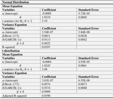
Table-2. Unrestricted GARCH (1,1) output for S&P500 INDEX

(Intercept) -0.0005 5.73E-05

1.0219 0.0069

(intercept) 3.54E-07 3.84E-08

(Resi(-1)^2) 0.0811 0.0038

(GARCH(-1)) 0.9113 0.0042

0.9925

R-squared 0.8397

b. t-distribution Mean Equation

(Intercept) -0.0004 4.93E-05

1.0245 0.0061

(intercept) 3.01E-07 6.55E-08

(Resi(-1)^2) 0.0574 0.0073

(GARCH(-1)) 0.9374 0.0068

0.9989

Adjusted R-squared 0.8390 Source: Developed by the authors

(7)

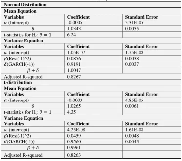
Table-3. Unrestricted GARCH (1,1) output for DAX INDEX

(Intercept) -0.0005 5.31E-05

1.0343 0.0055

(intercept) 1.05E-07 1.75E-08

(Resi(-1)^2) 0.0856 0.0038

(GARCH(-1)) 0.9191 0.0037

1.0047

Mean Equation

(Intercept) -0.0003 4.85E-05

1.0265 0.0061

(intercept) 4.25E-08 1.61E-08

(Resi(-1)^2) 0.0459 0.0048

(GARCH(-1)) 0.9560 0.0043

0.9961

Adjusted R-squared 0.8263

Source: Developed by the authors

Table 3 presents the empirical results for the DAX index. When the errors of the mean equation are normally distributed, we can see that is significantly upward biased at 95% confidence level, providing evidence of a clear overreaction in terms of level dependence in the volatility of the index. There is a slight overreaction as the parameters ( in this model. However, we can see that this overreaction is absorbed when the errors follow a t-distribution. Here also, we can see a clear existence of level dependence as the estimator is significantly upward biased at 95% confidence level. The model is able to explain around 83% variation making it a sound econometric model.

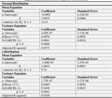
Table 4 presents the results for GARCH (1, 1) model for the FTSE100 index. From the table, we can infer from the significant t-statistics at 95% confidence level that is upward biased for FTSE100 index, under both probability distributions. Furthermore, in both the panels, we can clearly see that the parameter ( is significantly less than1 as expected. The model also has a high R-squared of 84%.

(8)

Table-4. Unrestricted GARCH (1,1) output for FTSE100 INDEX

(Intercept) -0.0002 6.31E-05

1.0819 0.0066

(intercept) 4.65E-07 3.11E-08

(Resi(-1)^2) 0.0879 0.0025

(GARCH(-1)) 0.9001 0.0034

0.9888

Mean Equation

(Intercept) -4.80E-05 5.37E-05

1.0655 0.0067

(intercept) 1.72E-07 4.27E-08

(Resi(-1)^2) 0.0465 0.0054

(GARCH(-1)) 0.9498 0.0053

0.9963

Table-5. ARCH LM Heteroscedasticity test

a. Normal Distribution

NIFTY S&P500 DAX FTSE100

F-Statistics 0.0006 0.0043 2.9759 0.2311

p-Value 0.9811 0.9478 0.0845 0.6306

t-Distribution

F-Statistics 0.0027 0.2322 6.6196 0.04642

p-Value 0.9582 0.6299 0.0101 0.8294

Table 5 presents two set of results. The first panel provides the test results for ARCH LM Heteroscedasticity test, when errors follow normal distribution. We can infer that none of the F-statistics are significant at 95% confidence level for any of the four indices under study. Similar is true in the case when error follow t-distribution as can be seen from the second panel of the table. Therefore, we can conclude that there are no residual ARCH effects in any of the models and that our volatility model was successful in capturing the same.

4.2. GARCH (1, 1) Model with IGARCH Restrictions

(9)

The results for the various indices are shown through Table 6-9.

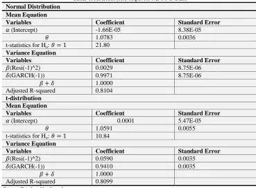
Table-6. IGARCH (1,1) output for NIFTY INDEX

Mean Equation

(Intercept) -1.66E-05 8.38E-05

1.0783 0.0036

t-statistics for Ho: 21.80

(Resi(-1)^2) 0.0029 8.75E-06

(GARCH(-1)) 0.9971 8.75E-06

1.0000

b. t-distribution

Mean Equation

(Intercept) 0.0001 5.47E-05

1.0591 0.0055

(Resi(-1)^2) 0.0590 0.0035

(GARCH(-1)) 0.9410 0.0035

1.0000

Table 6 presents the empirical result for the IGARCH (1, 1) model for the NIFTY index. We can see that there is significant upward bias in the covariance estimator at 95% confidence level when errors follow either normal or t-distribution. This clearly provides evidence for the existence of level dependence in the volatility of stock returns as also seen in Table 1 in Section 4.1.

Table-7. IGARCH (1,1) output for S&P500 INDEX

Mean Equation

(Intercept) -0.0006 4.48E-05

1.0236 0.0051

(Resi(-1)^2) 0.0492 0.0010

(GARCH(-1)) 0.9508 0.0010

1.0000

Mean Equation

(Intercept) -0.0004 4.50E-05

1.0238 0.0059

(Resi(-1)^2) 0.0325 0.0028

(GARCH(-1)) 0.9675 0.0028

1.0000

(10)

Table 7 provides empirical results for IGARCH (1, 1) model for S&P500 index. From the output panel, under the assumption of a normal distribution, we can see that the t-statistics is significant at 95% confidence level, thereby making upward biased. Similar results can be observed under the assumption of a t-distribution. The model has a high goodness of fit as evidenced by an R-squared of 84%.

Table-8. IGARCH (1,1) output for DAX INDEX

Mean Equation

(Intercept) -0.0005 3.50E-05

1.0349 0.0047

(Resi(-1)^2) 0.0614 0.0023

(GARCH(-1)) 0.9386 0.0023

1.0000

Mean Equation

(Intercept) -0.0003 4.35E-05

1.0268 0.0033

(Resi(-1)^2) 0.0379 0.0032

(GARCH(-1)) 0.9621 0.0032

1.0000

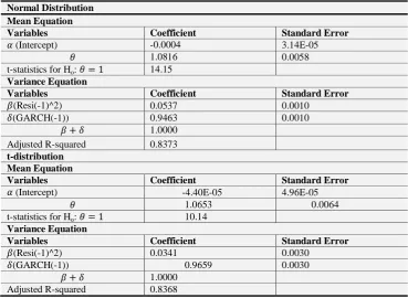
Table-9. IGARCH (1,1) output for FTSE100 INDEX

Mean Equation

(Intercept) -0.0004 3.14E-05

1.0816 0.0058

(Resi(-1)^2) 0.0537 0.0010

(GARCH(-1)) 0.9463 0.0010

1.0000

Mean Equation

(Intercept) -4.40E-05 4.96E-05

1.0653 0.0064

(Resi(-1)^2) 0.0341 0.0030

(GARCH(-1)) 0.9659 0.0030

1.0000

(11)

From the empirical results for the DAX index presented in Table 8, we can clearly see that there is a significant upward bias for DAX index against the null hypothesis at 95% confidence level. The IGARCH restriction ensures persistence in the volatility of index. These results conform to our earlier findings that there exists an overreaction in the stock returns that can be attributed to level dependence in volatility of stock returns. The results hold true in the case of both the probability distributions.

From Table 9, we can infer that when we assume errors to follow a normal distribution, the covariance estimator as evidenced by the significant t-statistics at 95% confidence level. The same holds true under the assumption of a student’s t-distribution for the errors. The model is also able to explain 84% variation in variables.

4.2. Testing for residual ARCH effects: Once again, using the ARCH LM Heteroscedasticity test with 1 lag, we test to identify the presence of any residual ARCH effects in our model. The results of the same are presented in Table 10.

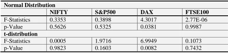
Table-10. ARCH LM Heteroscedasticity test

NIFTY S&P500 DAX FTSE100

F-Statistics 0.3353 0.3898 4.3017 2.77E-06

p-Value 0.5626 0.5325 0.0381 0.9987

t-distribution

F-Statistics 0.0005 1.9716 6.9949 0.1073

p-Value 0.9823 0.1603 0.0082 0.7432

From Table 10, we can see that when errors follow normal distribution or a student’s t-distribution, for all the indices in general, none of the F-statistics is significant at 95% confidence level. This shows that there are no residual ARCH effects in our model.

To sum up the findings of the empirical study, we have ample evidence that the estimator is upward biased for all the indices under study. That is to say, empirically speaking the proposed covariance estimator We can attribute such an overreaction in stock indices to the level dependence in the volatility of stock returns where by intraday local volatility of stock price is impacted by intraday level of stock prices.

These findings agree with those of our earlier study (Lakshmi and Maheswaran, 2016) where we find a significant upward bias for the same stock indices under study. We have seen that random walk model cannot explain this phenomenon. The Constant Elasticity of Variance (CEV)1 specification can capture the level dependence that makes the estimator upward biased as seen in the data. We show that it is possible to isolate the effect of intraday level dependence in stock prices using our estimator.

In this study, it is the same CEV effect that comes into play that makes the estimator upward biased. We show that it is also possible to estimate covariance using daily high-low prices by making use of the conventional regression approach. The GARCH (1, 1) or the IGARCH (1, 1) model is aptly able to capture this phenomenon using our proposed covariance estimator.

1_{CEV explains the relationship between share price and volatility. It was developed by}_{Cox (1996}₎_._{We found in our earlier paper that the CEV specification allows for}

(12)

5. CONCLUSION

In this paper, we propose an alternative approach to work with the new covariance estimator based on daily high-low prices that we had proposed in our earlier study (Lakshmi and Maheswaran, 2016). Using the GARCH (1, 1) and IGARCH (1, 1) models, we empirically examine four major stock indices and find that the estimator is upward biased for all the indices under study. Furthermore, we find that there are no residual ARCH effects in the models. In the earlier study, we had proved that random walk behavior cannot explain this overreaction in stock returns. Therefore, we had attributed this phenomenon to the level dependence in the volatility of stock returns. We find that it is the same Constant Elasticity of Variance (CEV) effect that comes into play here that makes the estimator upward biased as seen in the data. Thus we show that one can adopt a regression based approach to capture the level dependence and the CEV effect, thus making this exercise universally applicable.

Funding: This study received no specific financial support.

Competing Interests: The authors declare that they have no competing interests.

Contributors/Acknowledgement: All authors contributed equally to the conception and design of the study.

REFERENCES

Alberg, D. and R. Shalit, 2008. Estimating stock market volatility using asymmetric garch models. Applied Financial Economics,

18(15): 1201–1208.

Alizadeh, S., M. Brandt and F. Diebold, 2002. Range-based estimation of stochastic volatility models. Journal of Finance, 57(3):

1047–1091.

Andersen, T. and J. Lund, 1997. Estimating continuous-time stochastic volatility model of the short-term interest rate. Journal of

Econometrics, 77(2): 343–377.

Bali, T., 2003. Modeling the stochastic behavior of short-term interest rates: Pricing implications for discount bonds. Journal of

Banking and Finance, 27(2): 201–228.

Ball, C. and W. Torous, 1984. The maximum likelihood estimation of security-prices volatility: Theory, evidence, and an

application to option pricing. Journal of Business, 57(1): 97-112.

Bollerslev, T., 1986. Generalized autoregressive conditional heteroscedasticity. Journal of Econometrics, 31(3): 307–337.

Bollerslev, T., R. Chou and F. Kroner, 1992. Arch modeling in finance. Journal of Econometrics, 52(1): 5–59.

Brandt, M. and C. Jones, 2006. Volatility forecasting with range-based EGARCH models. Journal of Business and Economics

Statistics, 24(4): 470-486.

Brenner, R., R. Harjes and K. Kroner, 1996. Another look at models of the short-term interest rate. Journal of Financial and

Quantitative Analysis, 31(1): 85–107.

Cox, J.C., 1996. The constant elasticity of variance option pricing model. Journal of Portfolio Management Special Issue, 23(5):

15–17.

Engle, R., 1982. Autoregressive conditional heteroscedasticity with estimates of the variance of United Kingdom inflation.

Econometrica, 50(4): 987–1007.

Engle, R. and A. Patton, 2001. What good is a volatility model? Quantitative Finance, 1(2): 237–245.

Garman, M. and M. Klass, 1980. On the estimation of security price volatilities from historical data. Journal of Business, 53(1):

67–78.

Kalu, O., 2010. Modelling stock returns volatility in Nigeria using GARCH models. Proceeding of International Conference on

Management and Enterprise Development, University of Port Harcourt Nigeria, 1(4): 5-11.

Koedijk, K., F. Nissen, P. Schotman and C. Wolff, 1997. The dynamics of short-term interest rate volatility reconsidered.

(13)

Kunitomo, N., 1992. Improving the Parkinson method of estimating security price volatil¬ities. Journal of Business, 65(2): 295–

302.

Lakshmi, P. and S. Maheswaran, 2016. A new statistic to capture the level dependence in the volatility of stock prices.

Unpublished Working Paper, IFMR, Chennai.

Magdon, I.M. and A. Atiya, 2003. A maximum likelihood approach to volatility estimation for a Brownian motion using high, low

and close price data. Quantitative Business, 3(5): 376–384.

Nelson, D., 1990. Stationarity and persistence in the GARCH(1,1) model. Econometric Theory, 6(3): 318–344.

Nelson, D., 1991. Conditional heteroscedasticity in asset returns: A new approach. Econometrica, 59(2): 347–370.

Parkinson, M., 1980. The extreme value method for estimating the variance of the rate of return. Journal of Business, 53(1): 61–

65.

Rogers, L. and S. Satchell, 1991. Estimating variance from high, low and closing prices. Annals of Applied Probability, 1(4): 504–

512.

Rogers, L. and F. Zhou, 2008. Estimating correlation from high, low, opening and closing prices. Annals of Applied Probability,

18(2): 813–823.

Shamiri, A. and Z. Isa, 2009. Modeling and forecasting volatility of the Malaysian stock markets. Journal of Mathematics and

Statistics, 5(3): 234–240.

Shin, J., 2005. Stock returns and volatility in emerging markets. International Journal of Business and Economics, 4(1): 31–43.

Shu, J.H. and J.E. Zhang, 2006. Testing range estimators of historical volatility. Journal of Futures Markets, 26(3): 297–313.

Stephan, F.G., 1996. Modelling the conditional distribution of interest rates as a regime switching process. Journal of Financial

Economics, 42(1): 27–62.

Yang, D. and Q. Zhang, 2000. Drift-independent volatility estimation based on high, low, open, and closing prices. Journal of

Business, 73(3): 477–491.