Dispersion representation of the D-term form factor in deeply virtual Compton scattering

Dispersion representation of the D-term form factor in deeply

vir-tual Compton scattering

B. Pasquini1,a

1_{Dipartimento di Fisica, Università degli Studi di Pavia, Pavia, Italy,}

and Istituto Nazionale di Fisica Nucleare, Sezione di Pavia, Pavia, Italy

Abstract. We review the dispersion relation formalism for the deeply virtual Compton scattering amplitudes, and derive a dispersive representation of the D-term form factor, using unsubtractedt-channel dispersion relations. Results for the D-term form factor as function oftas well as att=0 are shown in comparison with available model predictions and phenomenological parametrizations.

1 Introduction

Dispersion relations (DRs) provide an useful framework to connect different observables and to extract nucleon structure quantities. In particular, DRs for Compton scattering processes, with both real and virtual photons, had wide applications for the prediction and extraction from experimental data of low-energy properties of hadron systems [1–5]. More recently, the dispersion formalism has been extended to describe the virtual Compton scattering process in the deep inelastic region [6–12]. In particular, it was shown that the amplitudes for deeply virtual Compton scattering (DVCS) satisfy subtracted DRs at fixedtwith the subtraction function defined by the D-term form factor [6–8]. The D term was originally introduced to complete the parametrization of the generalized parton distributions (GPDs) in hard exclusive reactions in terms of double distributions, and restore the polynomiality property of the singlet moments of unpolarized GPDs [13]. This term turned out to be a crucial contribution in the phenomenological description of DVCS observables, where different forms have been assumed with parameters tuned to DVCS data [9, 14].

Here we review the dispersive representation of the D-term form factor in terms of DRs in the t-channel, as recently proposed in Ref. [15]. The advantage of this dispersive representation is to provide a microscopic interpretation of the physical content of the D-term form factor in terms of t-channel exchanges with the appropriate quantum numbers.

In Section 2, we review the derivation of thes-channel subtracted dispersion relations for the DVCS amplitudes. In Section 3, we derivet-channel DRs for the D-term form factor, and give the ingredients for the explicit calculation, by saturating the unitarity relation for thet-channel amplitudes with two-pion intermediate states. We then discuss the dispersive predictions for the D-term form factor in Section 4, and we conclude summarizing our results.

a_{e-mail: [email protected]}

C

s

γ∗_{(q)N(p)→γ(q)N(p), (1)}

where the variables in brackets denote the four-momenta of the participating particles. The familiar Mandelstam variables ares=(p+q)2_,t=(q−q)2_,u=(q−p)2_{,and are constrained bys+u+t=} 2M2

N−Q2, withMNthe nucleon mass andQ2=−q2. We will consider the Bjorken regime, where the

photon virtualityQ2_{andsare large, and−ts,Q}2_. The DVCS amplitude reads

Tλ_γλ

N,λγλN =εμ(q, λγ)ε∗ν(q, λγ)H μν λ

N,λN, (2)

whereελγ(ε∗λ_γ) is the polarization vector of the incoming virtual (outgoing real) photon and the DVCS

tensor is defined as the nucleon matrix element of theT-product of two electromagnetic currents:

Hλμν

N,λN =−i

d4x e−i(q·x)N(p, λN)|T[Jμ(x)Jν(0)|N(p, λN), (3)

whereλN(λ_N) is the helicity of the incoming (outgoing) nucleon.

The DVCS amplitude for unpolarized nucleon and at leading order inQcan be parametrized as

Tλ_γλ

N,λγλN =εμ(q, λγ)ε

∗

ν(q, λγ) (−gμν_⊥)

2

× ⎡ ⎢⎢⎢⎢⎢

⎢⎣u¯(p, λN)γ·n u(p, λN)

q

e2qCq−u¯(p, λN)u(p, λN)

1 MN

q

e2qFq ⎤ ⎥⎥⎥⎥⎥

⎥⎦, (4)

where we introduced the lightlike vectornμ =1/(√2P+)(1,0,0,−1), withP = (p+p)/2, and the symmetric tensorgμν_⊥ =gμν−nμp˜ν−nνp˜μ, with ˜pμ=P+/√2(1,0,0,1). Furthermore, the light-front component for a generic four-vectoraμis defined as (a0_+a3_)/√_{2. In Eq. (4), the invariant amplitudes} Cq_andFq_{are given by}

Cq(ξ,t)=

1

−1 dxH

(+)_{(x, ξ,t)+E}(+)_{(x, ξ,t)} x−ξ+i , F

q_(ξ,t)=

1

−1 dxE

(+)_{(x, ξ,t)}

x−ξ+i , (5)

with the skewedness variable defined asξ = Q2_/(2s+Q2_{). H}(+)_{(x, ξ,t) =H}q_{(x, ξ,t)−H}q_{(−x, ξ,t)}

denotes the singlet (C= +1) combination of nucleon helicity-conserving GPDs, and analogously for the nucleon helicity-flip GPDE(+)_{. The invariant amplitudes and the GPDs in Eq. (5) depend also on} the renormalization scaleμ2, which is not explicitly displayed, and it is identified with the hard scale of the processQ2_.

In the following we will consider the invariant amplitude Fq _{in theν−t plane at fixed Q}2_{, with}

ν=(s−u)/4MN =Q2/4MNξ. In this plane,Fqsatisfies the following fixed-tsubtracted relation [6, 11]

Fq(ν,t)=Fq(0,t)+ν 2

π

_∞

ν0 dν2

ν2

ImFq_(ν,t)

ν2_−ν2 , (6)

where the lower limit of integration isν0=Q2/4MNand the nucleon pole term residing in this point

may be considered separately. Following Refs. [6, 8], the subtraction functionFq_{(0,t) can be related}

to the D-term form factorDq_{(t) [13] as follows}

Fq(0,t)=2

₊1

−1 dzD

q_(z,t)

1−z =4D

3

_t

-channel dispersion relations for the D-term form factor

The dispersive representation for the D-term form factor Dq_{(t) of Eq. (7) is obtained by applying}

unsubtracted DRs, this time in the variablet:

Fq(0,t)=1_π

_+∞

4m2 π

dtImtF

q_(0,t)

t−t + 1

π

₋a

−∞ dt

ImtFq(0,t)

t−t . (8)

The imaginary part in the integral from 4m2

π →+∞in Eq. (8) is saturated by the possible intermediate states for thet-channel process, which lead to cuts along the positive-taxis. For low values oft, the t-channel discontinuity is dominated byππintermediate states.

The second integral in Eq. (8) extends from−∞to−a = −2(m2

π +2MNmπ)−Q2. As we are

inter-ested in evaluating Eq. (8) for largeQ2_{values and small (negative) values oft(|t| a), the integral}

from−∞ → −a is suppressed, and will be neglected in this work. Consequently, we shall saturate

the integral in Eq. (8) by the contribution ofππintermediate states, which turns out to be a good approximation for smallt.

We start by decomposing thet-channel helicity amplitude forγ∗γ→_NN¯ _{into a partial wave series,}

Tλt_N¯λN, λγλγ(ν,t) =

J

2J+1 2 T

J(γ∗_γ→NN¯) λNλN¯, λγλγ (t)d

J

ΛNΛγ(θt), (9)

whereΛγ =λγ−λγ,ΛN =λN−λ_N¯, andd_ΛJ

NΛγare Wignerd-functions. As described in Ref. [15], the unitarity relation for the the partial-wave amplitudes in thet-channel, with only theππintermediate states, reads

2 ImTλJN¯(γλN∗, λγ→γλNγN¯)(t)= 1 (8π)

pπ

√

t

T_ΛJγ(γ∗γ→ππ)(t) T

J(ππ→N_N¯)

ΛN (t)

∗

, (10)

whereTJ(γ∗γ→ππ)_andTJ(ππ→N_N¯)_{are the partial-wave amplitudes for theγ}∗_{γ→ππand theππ→NN¯} subprocesses, respectively.

The partial-wave amplitudes T_ΛJ_N(ππ₌0→NN¯) are related to the amplitudes f+J(t) of Frazer and Fulco [16] by the relation

T_ΛJ_N(ππ₌₀→NN¯)(t) = 16π pt (pt pπ)

J_fJ

+(t). (11)

The reactionγ∗γ → ππat largeQ2_{and smalltcan be described in a factorized form [17, 18], as the} convolution of a short-distance contribution,γ∗γ→qq¯, perturbatively calculable, and nonperturbative matrix elements describing the exclusive fragmentation of aqq¯pair into two pions. These nonper-turbative functions correspond to two-pion generalized distribution amplitudes (GDAs). In particular, one finds

T_ΛJ_γ(γ₌∗₀γ→ππ)(t)=

q

e2qTJ

(γ∗_γ→qq¯)

Λγ=0 (t) (12)

with

T_ΛJ_γ(γ₌∗₀γ→qq¯)(t)= 6 2J+1

n=max(1,J−1) odd

1

0

dz(2z−1) ˜BnJ(t)C(3/2)n (2z−1), (13)

whereC(3/2)n are Gegenbauer polynomials, and ˜Bq_nl are expansion coefficients of the GDA

express the 2πt-channel contribution to ImtFq(ν=0,t) as

ImtFq(ππ) =−M√Npπ

t p2

t

J

even 2J+1

2 (−1)

J/2(J−1)!!

J!! (ptpπ)

J_TJ(γ∗_γ→qq¯)

Λγ=0 f+J∗(t). (14)

For the numerical estimate, we restrict ourselves to theS- andD-wave contributions in Eq. (14). The partial-wave amplitudes of theππ → N_N¯ _{subprocess are taken from [21]. The two-pion GDAs are} calculated through DRs using the Omnès representation [19, 20, 22–24]. The results for theS- and D-wave coefficients, forn=1 in the Gegenbauer expansion of (13), read

˜

B10(t)=−B12(0)3C−β 2

2 f0(t), B12˜ (t)=β 2

B12(0)f2(t), (15)

where the Omnès functions f0,2 can be related toππphase-shiftsδ0

0,2(t) using Watson theorem and dispersion relations [19]. In Eq. (15), the constantCis taken from Ref. [20], using the estimate from the instanton model [25] at low energies,C=1+bm2

π+O(m4π) withb≈ −1.7 GeV−2, while the coeffi-cientB12(0) is obtained using the crossing relations between the quark 2πDA’s and the corresponding parton distributions in the pion, i.e.

B12(0)= 10 9

dx x 1 Nf

f

[qπf(x)+q¯πf(x)]. (16)

As final result, taking into account only the contribution withJ=0 andJ=2, Eq. (14) simplifies to

ImtFq(ππ)=

3MNpπ

2√t p2

t

B12(0)(3C−β2)f0(t)f+0∗(t)+(pπpt)2β2f2(t)f+2∗(t)

. (17)

In Eq. (17), the dependence on the renormalization scale enters only through the coefficientBq₁₂ eval-uated att =0, and therefore is disjoined from thetdependence of the amplitude. Furthermore, the coefficientsBq12evolve in the same way as the quark momentum fraction in the pion, in accordance with Eq. (16).

We note that the restriction ton = 1 in the Gegenbauer expansion of the GDAs corresponds to a similar restriction for the D-term form factor. As a matter of fact, the D-termD(z,t) in Eq. (7) can be expanded in terms of Gegenbauer polynomialsC3/2n , leading to the following representation for the

D-term form factorDq(t)=∞_n=1

noddd

q

n(t).Accordingly, the numerical results shown in the next section

are for the contributiondq₁(t).

4 Results

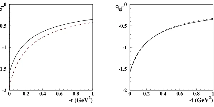
In Fig. 1 we present the dispersive predictions ford1Q=

qd1q(t) as function oft, with the sum over flavors restricted to up and down quarks. The solid and dashed curves are obtained using as input in Eq. (16) the parametrization of the pion distributions atQ2 _{= 4 GeV}2 _{from Refs. [26] and [27],} respectively. The different inputs for the pion distributions change the results by an overall normal-ization factor, without affecting thetdependence. As outlined above, theQ2_{dependence enters only} through the quark momentum fraction of the pion, which changes only by a few percent in the range ofQ2 _{=[1,10] GeV}2_{. Att=0, we findd}Q

1 =−1.59 andd

Q

-2 -1.5 -1 -0.5 0

0 0.2 0.4 0.6 0.8 1

-t (GeV2) d1

Q

-2 -1.5 -1 -0.5 0

0 0.2 0.4 0.6 0.8 1

-t (GeV2) d 1

Q

Figure 1.d1Qas function oft, atQ

2_{=4 GeV}2_{, obtained with the quark distributions in the pion}

qπf from Ref. [26]

(solid curve) and Ref. [27] (dashed curve). Right panel:tdependence of the DR results ford1Q(t) withq f

πfrom

Ref. [26] (solid curve) in comparison with the function in Eq. (18) (dashed curve).

with effective light-front wave functions from a Regge-improved diquark model [30],d1q(0)=−2.01. dQ₁(t) is particularly interesting, as it enters in the parametrization of the quark part of the energy mo-mentum tensor of QCD, and provides information on how strong forces are distributed and stabilized in the nucleon [31]. In all theoretical studies so far, as well as in the present dispersive calculation, d1Q(t) at zero-momentum transfert = 0 is found to have a negative sign. The negative value of this constant has a deep relation to the spontaneous breaking of the chiral symmetry in QCD [31, 32], and has also an appealing connection with the criterion of stability of the nucleon [28].

In most of phenomenological studies of DVCS, the t dependence of D-term form factor is parametrized by a dipole function [14]. However, the dispersive results favor a different functional form, as shown in the right panel of Fig. 1 where we compare the result ford1Qas function oftwith the following parametrization

FD=

d₁Q(0) [1−t/(αM2

D)]α

,withMD=0.487 GeV andα=0.841. (18)

5 Conclusions

Q2_{dependence of the D-term form factor are disjoined. Thet-dependence is not trivial and does not} follow a dipole behavior as normally assumed in phenomenological parametrizations. The value at t=0 is also compatible with estimates in chiral-quark soliton model and a Regge-improved diquark model. TheQ2_{dependence enters only in the normalization point att =0, which is proportional to} the firstx-moment of the flavor-singlet pion PDFs.

References

[1] D. Drechsel, B. Pasquini and M. Vanderhaeghen, Phys. Rept.378, 99 (2003).

[2] B. Pasquini, M. Gorchtein, D. Drechsel, A. Metz and M. Vanderhaeghen, Eur. Phys. J. A11, 185 (2001); Phys. Rev. C62, 052201 (2000).

[3] D. Drechsel, M. Gorchtein, B. Pasquini and M. Vanderhaeghen, Phys. Rev. C61, 015204 (1999). [4] B. Pasquini, D. Drechsel and M. Vanderhaeghen, Phys. Rev. C76, 015203 (2007).

[5] B. Pasquini, D. Drechsel and S. Scherer, Phys. Rev. C77, 065211 (2008). [6] I. V. Anikin and O. V. Teryaev, Phys. Rev. D76, 056007 (2007).

[7] O. V. Teryaev, hep-ph/0510031.

[8] A. V. Radyushkin, Phys. Rev. D83, 076006 (2011).

[9] K. Kumericki, D. Müller and K. Passek-Kumericki, Nucl. Phys. B794, 244 (2008). [10] D. Müller and K. M. Semenov-Tian-Shansky, Phys. Rev. D92, no. 7, 074025 (2015). [11] M. Diehl and D. Y. Ivanov, Eur. Phys. J. C52, 919 (2007).

[12] M. V. Polyakov and M. Vanderhaeghen, arXiv:0803.1271 [hep-ph]. [13] M. V. Polyakov and C. Weiss, Phys. Rev. D60, 114017 (1999).

[14] M. Guidal, H. Moutarde and M. Vanderhaeghen, Rept. Prog. Phys.76, 066202 (2013). [15] B. Pasquini, M. V. Polyakov and M. Vanderhaeghen, Phys. Lett. B739, 133 (2014). [16] W. R. Frazer and J. R. Fulco, Phys. Rev.117, 1603 (1960).

[17] M. Diehl, T. Gousset, B. Pire and O. Teryaev, Phys. Rev. Lett.81, 1782 (1998). [18] M. Diehl, T. Gousset and B. Pire, Phys. Rev. D62, 073014 (2000).

[19] M. V. Polyakov, Nucl. Phys. B555, 231 (1999).

[20] N. Kivel, L. Mankiewicz and M. V. Polyakov, Phys. Lett. B467, 263 (1999).

[21] G. Höhler, Pion-Nucleon Scattering, Landolt-Börnstein, Vol. I/9b2, edited by H. Schop-per Springer, Berlin, 1983.

[22] B. Lehmann-Dronke, P. V. Pobylitsa, M. V. Polyakov, A. Schäfer and K. Goeke, Phys. Lett. B

475, 147 (2000).

[23] B. Lehmann-Dronke, A. Schäfer, M. V. Polyakov, K. Goeke, Phys. Rev. D63, 114001 (2001). [24] N. Warkentin, M. Diehl, D. Y. Ivanov and A. Schafer, Eur. Phys. J. A32, 273 (2007).

[25] M. V. Polyakov and C. Weiss, Phys. Rev. D59, 091502 (1999). [26] J. F. Owens, Phys. Rev. D30, 943 (1984).

[27] M. Gluck, E. Reya and A. Vogt, Z. Phys. C53, 651 (1992).

[28] K. Goeke, J. Grabis, J. Ossmann, M. V. Polyakov, P. Schweitzer, A. Silva and D. Urbano, Phys. Rev. D75, 094021 (2007).

[29] C. Cebulla, K. Goeke, J. Ossmann and P. Schweitzer, Nucl. Phys. A794, 87 (2007). [30] D. Müller and D. S. Hwang, arXiv:1407.1655 [hep-ph].