Computational studies on ECE spectrum for ITER, in the presence of a small
fraction of non-thermals and radial resolution evolution for oblique view
P.V. Subhash1,a, Yashika Ghai2, Hitesh K. Pandya1, Amit K. Singh1, A. M. Begam3, and P. Vasu1
1ITER-India, Institute for Plasma Research, Gandhinagar, India 2GNDU, Amritsar, Punjab, India
3Kanchi Mamunivar Center for Post Graduate Studies, Poducherry, India
Abstract. In tokamaks, the temperature measurement using different techniques like Electron Cyclotron Emis-sion (ECE), Thomson scattering etc. shows differences because of various phenomena. The physical reasons for this are not entirely understood. Thus to have comprehensive understanding of these difference, the contribu-tion from each phenomenon needs to be individually understood. The phenomenon affecting radial temperature profile measurement includes harmonics overlap, relativistic down shifting, presence of non-thermals etc. For ITER like plasma, radial temperature profiles can be obtained from the first harmonics ordinary (O) mode or second harmonic extra-ordinary(X) mode of ECE spectrum. It is possible that, higher harmonics produced from the non-thermals can be relativistically downshifted to second harmonics and results a deviation in the measured temperature profile. We performed a parametric study on the e ffect of non-thermal electrons on measured ECE temperature for ITER scenario-2. All the numerical calculations reported in this paper are performed using NOTEC computer code which is capable of handling non-thermal populations. After proper validation of nu-merical methods using normal electron population (without non-thermals) a parametric study with non-thermals is performed. In the parametric study radial locations of non-thermals, energy of non-thermals and fraction of non-thermals are considered. This study is initially performed for normal view and later extended in to oblique views. The range of deviation of temperature over the examined parametric regime as well as the possible phys-ical reasons will be presented. The effect of parallel component of non-thermal energy is also examined. Finally results of one set of study for oblique view (where the detector is not exactly normal to the magnetic field) with non-thermal electrons are also presented. In ITER apart from an Electron Cyclotron Emission (ECE) detector placed normal to magnetic field an oblique view detector is planned to grab information about non-thermal electrons. Usefulness of such an additional detector for a better radial resolution is examined. The differences in the ECE spectrum from a tokamak plasma between a direct LOS (normal to toroidal magnetic field) and a slightly oblique LOS have been modelled. A typical ITER tokamak scenario has been chosen in this study. The intensities of radiation, as observable from the low-field side, covering the first harmonic O-mode spectral frequencies 105-230 GHz have been compared. The physical reasons for the code-predicted results, regarding the differences between the direct and oblique spectra, are elucidated. Finally, signatures of the presence of non-thermals from a comparison of normal view and oblique view are also examined.
1 Introduction
Electron Cyclotron Emission (ECE) measurement is con-sidered as one of the reliable techniques for radial elec-tron temperature(Te) measurement in tokamaks [1, 2]. A comprehensive review of physical and technical aspects are available from reference [1]. The frequency of emis-sion of ECE along the radial location can be calculated by using the local toroidal magnetic field strength in the corresponding locations. By measuring the ECE intensity for many relevant frequencies radial temperature profile can be obtained. The procedure of obtainingTethrough ECE measurement is well established in literature (See ref [1, 2] and references therein). For ITER the radial tem-perature information can be inferred from first harmonics
ae-mail: [email protected]
ordinary modes (O-modes) or second harmonics extra or-dinary modes (X-modes) [2, 3]. But for high temperature tokamaks like ITER the capabilities of this method is lim-ited by various effects like harmonic overlap, polarization scrambling, due to the deviation of electron populations from Maxwellian etc [4].
Many studies are reported on difference between mea-sured temperature using ECE and other techniques like Thomson Scattering(TS). G. Taylor reported a difference of 10-20 % between ECE and TS when heated with NBI at 10 KeV electron temperature [5]. JET with NBI heat-ing alone or with combination of ICRH found a discrep-ancy about 30 % at 12 KeV [6]. Recent experiments on JET to understand the discrepancy on heating method finds that some methods like ICRF do not show any dis-crepancy [7]. Another experiments at DIII-D and C-MOD
C
with electron temperature up to 8 KeV found out no ob-vious difference [8]. Hence it can be concluded that the difference in temperature measurement between ECE and other methods strongly depend up on heating methods as well as electron temperature. This is not well understood. ITER is expected to reach a temperature up to 25 KeV with strong electron-ion coupling. It is important to understand the ’deviation’ in the ECE measurement individually for direct electron heating (such as ECCD and ECRH) and ion heating (such as ICRH and NBI). Departure of the electron distribution from Maxwellian is considered as one possi-ble cause of this deviation. The electron populations can be deviated from Maxwellian because of the presence of super thermal electrons.
2 Radial resolution evaluation
2.1 Normal view
The calculations reported in this article are performed using a computer code NOTEC (NOn Thermal ECE). NOTEC code calculates measured ECE spectra using an-tenna pattern, reflection, refraction and non-thermal pop-ulations [9, 10].A burning H-mode ITER scenario-2 [11, 12] has been taken for these calculations. The major and minor radius of the ITER machine is 6.2 m and 2 m re-spectively. The detector is assumed to be at radius R=8.2 m, Z=0.76 m andφ=0.
For ITER, in principle the radial temperature can be deduced from first harmonics ordinary mode (O mode) and second harmonics extra ordinary mode (X-mode). Such
0 5 10 15 20 25
4.5 5 5.5 6 6.5 7 7.5 8
T(KeV)
Major radius(m) --> T(O)
--> T(X) T(in)-->
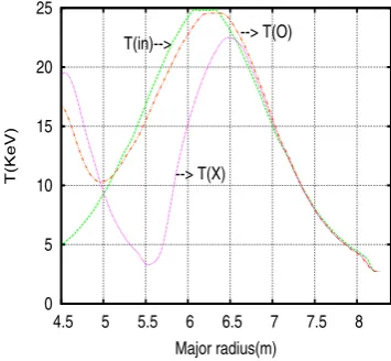
Figure 1.The input(T(in)) and calculated (with O-mode (T(O)) and X-mode (T(X))) temperature profiles.
kind of temperature profiles are calculated using NOTEC computer code. For the purpose of all the calculations re-ported in this article the ITER parameters and profiles are adapted from Ref [13]. The input and calculated tempera-ture profile from first harmonics O-mode and second har-monics X-mode is shown in figure 1.
The temperature calculated in the present study is in good agreement with previous studies reported in [4, 14].
From figure 1 it is clear that O-mode yields more reliable temperature profile can be obtained. Hence most of the calculations reported in this article is limited to O-mode unless otherwise specified.
2.2 Oblique view
In similar way, calculations are repeated for three cases of oblique view detector . Here the detector is assumed to be placed in an angle with respect to the normal to the mag-netic field in the toroidal plane. The three cases simulated here are for the angles 5◦,10◦ and 20◦.The obtained fre-quency spectrum for all three cases along with the spec-trum for normal view case is shown in figure 2. From the figure 2 it is clear that frequency spectrum for all the oblique cases are shifted from normal view spectrum. Fur-ther the amount of the shift is different for different view-ing angles. The frequency shift is due to Doppler shift, which modify the resonance condition into:
ω=n eB
me(γ−Nu) (1)
WhereNis the parallel component of refractive index and u ≡ P/m0cis parallel component of normalized electron momentum.
The usefulness of equation 1 is limited asNis func-tions of local plasma parameters. But the NOTEC code is capable to provide the location of emission for any fre-quency. This has been used for obtaining one to one cor-respondence between location of emission and frequency. The corresponding plot for the location of emission against frequency is shown in figure 3. Figure 3 is used to obtain the radial temperature profile for all the cases. In an ex-perimental situation also one need to adopt some methods to counter the shift in the oblique spectrum to obtain radial temperature profile. This is can be achieved either by us-ing numerical calculations or by locatus-ing the phenomena (for example fluctuations) from the normal view and ex-tract the properties of phenomena from both type of views. The second methodology is relevant only for understand-ing fluctuations or instabilities.
0 5 10 15 20 25
100 120 140 160 180 200 220
T(KeV)
f(GHz)
0° 5° 10° 20°
Figure 2.Obtained frequency spectrum for frequencies between 112 GHz to 220 GHz for various viewing angle.
100 120 140 160 180 200 220
4 4.5 5 5.5 6 6.5 7 7.5 8 8.5
f(GHz)
Major Radius (m)
Figure 3. The one to one correspondence between location of emission and frequency for various viewing angle. The curves from bottom to top are for 0◦, 5◦, 10◦and 20◦respectively.
3 Dependence of radial resolution and
localization of fluctuations on viewing
angle of ECE detector
3.1 Radial resolution
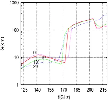
The radial resolution of ECE emission for a particular fre-quency for the purpose of the calculations reported here is defined as the radial thickness of emission between 5% to 95 % of the total intensity. In order to demonstrate this point we have shown an example of calculating width of emission (δr) for a frequency f=142GHz for the case of normal view in figure 4. From the figure 4 it is clear that the emission for this particular frequency is centered around a radial location of 6.3 and extent of emission (be-tween 5 % to 95 %) is be(be-tween 6.245 m and 6.360 . Hence the radial resolution of emission (δr) for 142 GHz is cal-culated as 11.5 cm. This process is repeated for all the frequencies ranging from 122GHz to 220GHz for normal
0 0.1 0.2 0.3 0.4 0.5 0.6 0.7 0.8 0.9 1
6 6.5 7 7.5 8 8.5
Normalized emission
Radius(m) --95%
--50%
--5%
Figure 4. Normalized emission as a function of radius for f=142GHz.
1 10 100 1000
125 140 155 170 185 200 215
δ
r(cm)
f(GHz) 20°
10° 5° 0°
Figure 5.Radial resolution for frequencies from 112 GHz to 220 GHz for various viewing angle.
im-portant as it cover the entire inboard side and center of the plasma.
4 Effect of a small amount of non-thermal
populations on T measurement for ITER
4.1 Parametric regime
In the parametric study reported here, the base profiles are seeded with super thermal electrons.
In order to include super thermals in the numerical scheme, we need to know location of the super thermals, energy of the super thermals and fraction of the super ther-mals relative to the background electron density. Ideally the above parameters can be obtained by solving Fokker-Plank equation for the corresponding heating or current drive processes, which in itself is a separate problem and is beyond the scope of this work. Nevertheless, we can un-derstand effect of super thermals on measured spectrum in a parametric study over a parametric regime of relevance. Such a study also provide insights of various physical as-pects of the problem within the frame work of the scanned parametric space. The present work attempt this method.
Three parameters considered in this study are location of the super thermals, fraction of the super thermals and perpendicular component of the energy of the super ther-mals.
We performed the calculations for three radial loca-tions which correspond to safety factor q=1, q=1.5 and q=2. These locations are selected because the proposed ECCD to stabilize various instabilities will be used at these locations. The super thermals are assumed to be dis-tributed in a drifted Maxwellian form [9] between the flux tubes bounded by 3 % around various ’q’ values and is further limited to a poloidal extend of 0.14 radian in the line of sight for the normal view. The fraction of super thermals are varied from 0.05% to 0.5%. As we see later in this article any amount of super thermal electrons lower than 0.05 has no effect on the temperature measurement. The upper limit of the of super thermals are set to 0.5 % be-cause logically we are not expecting more than this value. Even in JET the maximum possible fraction is about 0.12 % (see reference [15]). So at present we do not expect su-per thermal electrons more than 0.5 % in ITER.The energy range of super thermals are initially bracketed in a range between 100 KeV and 250 KeV.
4.2 Results of parametric study
In this section following results are included. Initially, re-sults of the parametric study is presented. This is followed by results for oblique view, where detector is placed at an angle with the magnetic field.
The effect of super thermals are analyzed in follow-ing way. Initial calculations are performed with-out super thermal to obtain the frequency spectrum. This is then fol-lowed by calculating spectrum with the inclusion of super thermals for the entire range of parametric regime. The ob-tained spectrum without super thermals are then subtracted
from the spectrum with super thermals to obtain the devi-ation as the function of frequencies and radial locdevi-ations. We call the difference of intensities with and without su-per thermals as ’deviation’ throughout rest of this article. The emission for the both first and second harmonics for ITER is relatively broad even without super thermals [4]. The broadening of emission regime for a particular fre-quency are expected to be higher for super thermals as the energy of the super thermals are much higher than that of the background electron. In other words even if a partic-ular radial point have unique magnetic field it is capable of emitting a broad range of frequencies. Further, the the frequency intensity spectrum will also be affected by the relativistic frequency down shifting as γ is greater than unity. Even if the frequency down shifting can be under-stood analytically the broadening of the emission drives the problem away from a simple analytical understanding. The problem will be further complicated by resonance, cutoffproperties of thermal plasma, which it self can limit the range of frequencies reaching the detector. Thus it is very difficult to reach a logical conclusion on the exact influence of these parameters in producing the deviation without the numerical calculations. Figure 6 and figure 7 show the emission spectrum of super thermals obtained using the methodology explained above for the case with locations of super thermal at q=1, q=1.5 and q=2. The figures 6,7 shows that emission from the super thermal ex-ist for almost all of the first harmonics frequencies. But the the intensity is more around the location of the super thermal and on the higher frequency side. It should be noted that no deviation is observed from the location of super thermals towards the detector side. This is because the corresponding frequencies are absorbed in between the location of emission and detector.
From the figures it can be noted that around two ra-dial locations the deviation is relatively more. Firstly in the radial location where the super thermals are present. This is due to broaden first harmonics emission around the characteristic frequency which is downshifted. As stated above in the side towards the detector the error is shielded by the abortion in the region between the emission loca-tion and detector. Second peak exist in the high field side due to the downshifted second harmonic emission, again characterized by the relativistic broadening.
These results are explained in details in the subsequent subsections . In each subsections the effect of each param-eters are analyzed and individually.
4.3 Fraction of super thermals
0 0.1 0.2 0.3 0.4 0.5 0.6
5 6 7 8
Deviation (%) Radius (m) (A) 0 0.5 1 1.5 2 2.5 3
5 6 7 8
Deviation (%) Radius (m) (B) 0 1 2 3 4 5 6
5 6 7 8
Deviation (%) Radius (m) (C) 0 2 4 6 8 10 12
5 6 7 8
Deviation (%) Radius (m) (D) 0 5 10 15 20 25
5 6 7 8
Deviation (%) Radius (m) (E) 0 5 10 15 20 25 30
5 6 7 8
Deviation (%)
Radius (m) (F)
Figure 6. Deviation of temperature as a function of radius with super thermals for various fractions and energies.The location of the super thermal population is at Q=1. In each plot three curves from bottom to top corresponds to 100 KeV, 150 KeV and 200 KeV respectively. Different curves A,B,C,D,E and F corresponds to fraction of super thermals 0.01,0.05,0.1,0.2,0.4 and 0.5 respectively.
0 0.5 1 1.5 2 2.5 3 3.5 4 4.5 5
5 6 7 8
Deviation (%) Radius (m) (1A) 0 1 2 3 4 5 6 7 8 9 10
5 6 7 8
Deviation (%) Radius (m) (1B) 0 2 4 6 8 10 12 14 16 18 20
5 6 7 8
Deviation (%) Radius (m) (1C) 0 0.5 1 1.5 2 2.5 3 3.5
5 6 7 8
Deviation (%) Radius (m) (2A) 0 1 2 3 4 5 6 7
5 6 7 8
Deviation (%) Radius (m) (2B) 0 2 4 6 8 10 12 14
5 6 7 8
Deviation (%)
Radius (m) (2C)
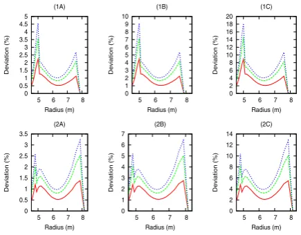
Figure 7. Deviation of temperature as a function of radius with super thermals for various fractions and energies. In each plot three curves from bottom to top corresponds to 100 KeV,150 KeV and 200 KeV. 1A : Q=1.5, Fraction=0.1, 1B :Q=1.5, Frac-tion=0.2, 1C :Q=1.5, Fraction=0.4, 2A :Q=2, Fraction=0.1, 2B :Q=2, Fraction=0.2, 2C :Q=2, Fraction=0.4
location of super thermal at q=1. In each graph three dif-ferent curves for different values of the energies are plotted together. Similar plots for the cases with location of the su-per thermals at q=1.5 and q=2 are presented in Figure 7. From these figures it can be noted that having more su-per thermals translates to more deviation, which is easy to understand as more super thermals results more emission. Another interesting point can be noted from the figures as for same value of the energy and location of super ther-mals the deviation is scaling linearly with the fraction of the super thermals. This point is further examined in the
0 0.5 1 1.5 2 2.5 3
5 6 7 8
Deviation (%)
Radius (m) (1A)
0 0.5 1 1.5 2 2.5 3 3.5 4 4.5
5 6 7 8
Deviation (%) Radius (m) (1B) 0 1 2 3 4 5 6
5 6 7 8
Deviation (%) Radius (m) (1C) 0 0.5 1 1.5 2 2.5
5 6 7 8
Deviation (%)
Radius (m) (2A)
0 0.5 1 1.5 2 2.5 3 3.5 4
5 6 7 8
Deviation (%)
Radius (m) (2C)
0 0.5 1 1.5 2 2.5 3 3.5 4 4.5 5
5 6 7 8
Deviation (%) Radius (m) (2C) 0 0.2 0.4 0.6 0.8 1 1.2 1.4
5 6 7 8
Deviation (%)
Radius (m) (3A)
0 0.5 1 1.5 2 2.5 3
5 6 7 8
Deviation (%)
Radius (m) (3B)
0 0.5 1 1.5 2 2.5 3 3.5
5 6 7 8
Deviation (%)
Radius (m) (3C)
Figure 8.Deviation of radial temperature as a function of radius for various parameters.Curves 1A, 1B and 1C is for case q=1 and energy=100, 150 and 200 respectively. The three curves, red line is for frac=0.1, green dot is for Deviation divided by 2 frac=0.2 and triangle is for deviation divided by 4 for frac=0.4. Others curves 2A, 2B,and 2C are for q=1.5 while 3A, 3B and 3C corresponds to q=2.
figure 8. In figure 8, for one value of energy and location of super thermals deviation are plotted as a function of the radial locations for three values of fractions 0.1% ,0.2 % and 0.4 %. The deviations are divided by two and four for the cases with fractions equal to 0.2 % and 0.4 % respec-tively. This is to understand how the deviations are related with fractions of the super thermals. Nine such plots are shown for 3 X 3 values of energy and locations.
4.4 Energy of super thermals
4.5 Location of super thermals
The simulations are repeated for 3 locations with q=1,q=1.5 and q=2. Moving from q=1 to q=2 we move more towards detector which is placed near the wall at low field side. The deviation in temperature for correspond-ing cases are shown in Figure 6 and Figure 7. Followcorrespond-ing points can be noted from the figures.
• From all the figures the deviation is minimum near the center. This is have a physical significance as the su-per thermal are least interfering the central temsu-perature measurement at least for the kind of super thermals stud-ied here
• For the same values of all other parameters, for the cases with higher ’q’ values deviation around the location of super thermals are increasing. In other words if the su-per thermals are present in the locations towards the wall at the low field side more deviation in the measured tem-perature around that region is noted. A possible expla-nation is given below. As we move away from the de-tector towards the high field side there is more chance that the radiation corresponding to the lower frequen-cies are getting absorbed between location of emission and detector.
• The peak near high field side almost remain same for the cases of q=1 and q=1.5 for same value of all other parameters. But the peak deviation in the high field side is considerably low for the case with location q=2. No possible scaling law is obtained for this case.
0.52 0.54 0.56 0.58 0.6 0.62 0.64 0.66 0.68 0.7 0.72
5 6 7
Radius (m) (1A)
0.35 0.4 0.45 0.5 0.55 0.6 0.65
5 6 7
Radius (m) (1B)
0.76 0.77 0.78 0.79 0.8 0.81 0.82 0.83 0.84 0.85 0.86
5 6 7
Radius (m) (1C)
0.5 0.55 0.6 0.65 0.7 0.75
5 6 7
Radius (m) (2A)
0.4 0.45 0.5 0.55 0.6 0.65
5 6 7
Radius (m) (2B)
0.77 0.78 0.79 0.8 0.81 0.82 0.83 0.84 0.85 0.86
5 6 7
Radius (m) (2C)
0.54 0.56 0.58 0.6 0.62 0.64 0.66 0.68 0.7 0.72 0.74 0.76
5 6 7
Radius (m) (3A)
0.4 0.45 0.5 0.55 0.6 0.65
5 6 7
Radius (m) (3B)
0.76 0.77 0.78 0.79 0.8 0.81 0.82 0.83 0.84 0.85 0.86
5 6 7
Radius (m) (3C)
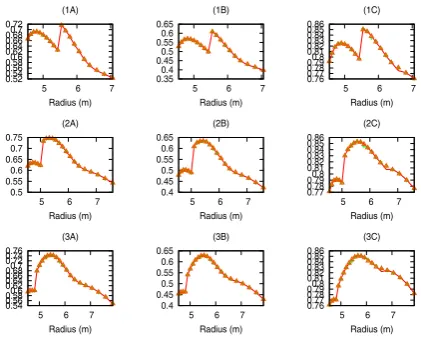
Figure 9.Deviation of radial temperature as a function of radial distance for various parameters. The curve 1A shows ratio of deviation for energy 100KeV and 150 KeV for all fractions ( line for frac=0.1 points for frac=0.2 and triangles for frac=0.4) for Q=1. 1B and 1C are for ratio of deviations for energies 150 KeV and 200 KeV and ratio between 100 KeV and 200 KeV. Similar curves are shown in 2A,2B and 2C for Q=1.5 and in 3A,3B and 3C for q=2.
References
[1] M. Bornatici, R. Cano, O.D. Barbieri, F. Engelmann, Nucl. Fusion23, 1153 (1983)
[2] E. de la Luna, J.E. Contributors, AIP Conference Proceedings988, 63 (2008)
[3] P.V. Subhash, Y. Ghai, S.K. Amit, A.M. Begum, Co-munnicated to Physics of Plasmas
[4] D. Bartlett,Physics issues of ECE and ECA for ITER, inDiagnostics for Experimental Thermonuclear Fu-sion Reactors, edited by P.E. Stott, G. Gorini, E. Sin-doni (Plenum, New York and London, 1996), p. 183 [5] G.T. et al,Electron cyclotron emission measurements on high beta TFTR plasmas, inProc. 9th Joint Work-shop on ECE and ECRH, edited by J.Lohr (World Scientific, Singapore, 1995, 1995), p. 485
[6] E. de la Luna, V. Krivenski, G. Giruzzi, C. Gowers, R. Prentice, J.M. Travere, M. Zerbini, Review of Sci-entific Instruments74, 1414 (2003)
[7] K.V. Beausang, S.L. Prunty, R. Scannell, M.N. Beurskens, M.J. Walsh, E. de La Luna, J.E. Contrib-utors, Review of Scientific Instruments82, 033514 ( 8) (2011)
[8] A. White, A. Hubbard, J. Hughes, P. Bonoli, M. Austin, A. Bader, R. Harvey, Y. Lin, Y. Ma, M. Reinke et al., Nuclear Fusion52, 063021 (2012) [9] R.M.J. Sillen, M. A.F.Allaart, W.J. Goedheer,
A. Kattenberg (Rijnhuizen report, 1987)
[10] H.V.D. Brand, M.D. Baar, N.L. Cardozo, E.Westerhof, Nuclear Fusion53, 013005 (2013) [11] T. Casper, Y. Gribov, A. Kavin, V. Lukash,
R. Khayrutdinov, H. Fujieda, C. Kessel, I. Organi-zation, I.D. Agencies, Nuclear Fusion 54, 013005 (2014)
[12] A.R. Polevoi, S.Y. Medvedev, V.S. Mukhovatov, A.S. Kukushkin, Y. Murakami, M. Shimada, A.A. Ivanov, Journal of Plasma and Fusion Research SERIES5, 82 (2002)
[13] I.P.B. Editors, I.P.E.G. Chairs, Co-Chairs, I.J.C. Team, P.I. Unit, Nuclear Fusion39, 2137 (1999) [14] S. Danani, H.K.B. Pandya, P. Vasu, M.E. Austin,
Fu-sion Science and Technology59, 651 (2011) [15] M. Brusati, D. Bartlett, A. Ekedahl, P. Froissard,