1

Evaluation of the Komlos Conjecture Using Multi-Objective

Optimization

Samir Brahim Belhaouari1 _{and and Randa AlQudah}2

1_{Division of Information & Computing Technology, College of Science and Engineering, Hamad Bin}

Khalifa University, [email protected].

2_{Electrical and Computer Engineering, Texas A&M University at Qatar, [email protected]}

ABSTRACT

Komlos conjecture is about the existing of a constant upper bound over the dimension 𝑛 of the function 𝐾(𝑛) defined by

𝐾(𝑛) = max

)*,,,,⃗,…,*+ ,,,,⃗1∈3*,,⃗∈ℝ0 0∶ 7*,,⃗ 7₈9: ;

0<_{@ min +,…,@0}∈{B:,:}0

7∑H 𝜀_E𝑉,,⃗_G EI: 7_JK.

In this paper, the function 𝐾(𝑛) is evaluated first for lower dimensions, 𝑛 ≤ 5, where it found that 𝐾(2) = √2, 𝐾(3) =√QR√::

S , 𝐾(4) = √3, and 𝐾(5) = UR√:UQ

V . For higher dimension, the function 𝑓(𝑛) = X𝑛 − ⌈ 𝑙𝑜𝑔Q(2HB:⁄ )⌉ is found to be a lower bound for the function 𝐾(𝑛), from where it is concluded 𝑛 that the Komlos conjecture is false i.e., the universal constant 𝑘 = max

H∈a 𝐾(𝑛) does not exist because of lim

c→J𝐾(𝑛) ≥ limc→JXlog(𝑛) − 1 = +∞.

Keywords:

Introduction

J. Komlos has made the following conjecture: For a given dimension 𝑛 , let 𝐾(𝑛) denote the minimum value such that: for any set of 𝑛 Vectors 𝑉,,,⃗ , … , 𝑉: ,,,⃗ ∈ ℝH H with 7𝑉,⃗E7_Q≤ 1 ,there exists weights 𝜀E= +1 𝑜𝑟 − 1 such that

lm 𝜀_E𝑉,⃗_E H

EI: l

J

≤ 𝐾(𝑛).

Kolmos has conjected the existence of a universal constant 𝐾 such that 𝐾(𝑛) ≤ 𝑘 for any dimension 𝑛 . The 𝑙Q and 𝑙J norms in ℝH are denoted by ‖. ‖Q and ‖. ‖J respectively.

This conjecture was referred by Joel Spencer [8] in 1994, where he linked kolmos Conjecture to Spencer’s famous Six Standard Deviation in 1985, see [9].

2 The main nontrivial result known, which is due to Joel Spencer [9], is that if 𝑘 ≤ 𝑛 then 7∑p 𝜀_E𝑉,⃗_E

EI: 7_J= 𝑂(log (𝑛)). The main result of D. Hajela [4] was very close to disprove the Komlos conjecture, where precisely he has proved the following theorem:

THEOREM 1. Let 𝑓(𝑛) be a function that’s goes to infinity when 𝑛 goes to infinity with 𝑓(𝑛) = 𝑂(𝑛) and let 0 < 𝜆 < 1/2. Then form 𝑛 ≥ 𝑛v (where 𝑛v depends only on 𝑛 and 𝜆) and any 𝐴 ⊆ {1, −1}H 𝑤𝑖𝑡ℎ |𝐴| ≤ 2H/~(H)_{, there are orthogonal vectors 𝑥}

:, … , 𝑥H 𝑖𝑛 𝑅H, ‖𝑥E‖Q≤ 1 for all 1 ≤ 𝑖 ≤ 𝑛, and such that ‖𝜀:𝑥:+ ⋯ + 𝜀H𝑥H‖J≥ exp „

𝜆 log log 𝑓(𝑛) log log log 𝑓(𝑛)…, for all (𝜀_:, … , 𝜀_H) ∈ 𝐴.

The previous theorem disproves the conjecture of Komlos over the set 𝐴 ⊆ {1, −1}H _{where |𝐴| ≤} 2H/~(H)_{. The proof of Theorem 1 is based on certain inequalities which arise in the geometry of convex} bodies [1], [10], and [2].

Komlos Conjecture is also related to discrepancy theory, paper of J.Becka and T.Fiala [6], where it states that for a global constant 𝐾 and for any 𝑚 × 𝑛 matrix 𝐴, whose columns are inside a unit ball, there exists a vector 𝑋 ∈ {−1, +1}H _{such that ‖𝐴𝑋‖}

J ≤ 𝐾.

The best progress in proving Komlos conjecture is a result given by Banaszczyk [11] who proved the bound

min

‰∈{B:,R:}0‖𝐴𝑋‖ ≤ 𝐾Xlog(𝑛) for a global constant.

This is the best known bound for Becka-Fiala conjecture as well [5].

Discrepancy is a challenging problem that has application in geometry, data analysis, and complexity theory. The books, J. Matousek [7], B. Chazelle [ 3], and J. Beck and V.T [5], provide references for a wide array of applications.

For lower dimension, the idea is to find a hypercube of minimum side of 2𝐾 , where all vertices formed by different combinations of the weights, ∑H_EI:𝜀_E𝑉,⃗_E , should be all inside the hypercube. Also It is not hard to show that √𝑛 is an upper bound for the function 𝐾(𝑛). The proof can be carried out by funding find a particular weights 𝜀E∗ such that all vectors 𝑉,,,⃗ , … , 𝑉: ,,,⃗ ∈ ℝH H with 7𝑉,,⃗ 7G _Q≤ 1, so

lm 𝜀_E∗ _𝑉,⃗ E H

EI: l

J

≤ 𝐾(𝑛) ≤ √𝑛.

The below boulets are the details of the proof: • We will prove first that 7∑ 𝜀_E∗ _𝑉,⃗

E H

EI: 7_Q≤ √𝑛 , which it is a sufficient condition to prove that 7∑HEI:𝜀_E∗𝑉,⃗E7_J≤ √𝑛 .

3 7𝜀_:∗_𝑉,⃗

:+ 𝜀Q∗𝑉,⃗Q 7_Q = ‹𝑉,⃗:+ 𝜀_Q∗ 𝜀_:∗𝑉,⃗Q ‹

Q

= Œ7𝑉,,,⃗7_{: Q}Q+ 7𝑉,,,⃗7_{Q Q}Q− 27𝑉,,,⃗7_{: Q}7𝑉,,,⃗7Q _Qcos•𝑉,,,,,⃗, 𝑉: ,,,,,⃗ •Q

≤ √2,

where the weight @8∗

@+∗ is chosen in order to have cos •𝑉,⃗:, 𝑉,⃗Q• ≥ 0. • If we suppose that 7∑ 𝜀_E∗ _𝑉,⃗

E HB:

EI: 7_Q ≤ √𝑛 − 1 , we need to prove that 7∑EI:HB: 𝜀E∗ 𝑉,⃗E+ 𝜀H∗ 𝑉,⃗H7_Q≤ √𝑛. Again by cosine rule, we can write the following:

lm 𝜀_E∗ _𝑉,⃗

E+ 𝜀H∗ 𝑉,⃗H HB:

EI:

l Q

≤ ‘7𝑉,,,⃗7H _Q Q

+ lm 𝜀_E∗ _𝑉,⃗ E HB: EI: l Q Q

≤ √1 + 𝑛 − 1

≤ √𝑛.

where the weight 𝜀H∗ is chosen in order to have cos •∑EI:HB: 𝜀E∗ 𝑉,⃗E, 𝜀H∗ 𝑉,⃗H• ≥ 0

• From the principle of induction proof, it is concluded that all vectors 𝑉,,,⃗ , … , 𝑉: ,,,⃗ ∈ ℝH H with 7𝑉,,⃗ 7G _Q≤ 1, the weights can find 𝜀E∗ such that

7∑ 𝜀_E∗ _𝑉,⃗ E H

EI: 7_Q ≤ √𝑛.

Since 7∑ 𝜀_E∗ _𝑉,⃗ E H

EI: 7_J≤ 7∑HEI: 𝜀E∗ 𝑉,⃗E7_Q, we can conclude that the function 𝐾(𝑛) has an upper bound of order √𝑛.

We can extend the Komlos conjecture statement to the below lemma, where it summarizes very interesting properties related to special vectors, 𝑉,,⃗G

∗

, 𝑖 = 1, … . , 𝑛, that cannot cancel each other further than 𝐾(𝑛) .

Lemma 1: Let 𝐶H _{be a set of vectors in ℝ}H _{have 𝑙}

Q norm at most 1, and we denote by 𝑉∗ as a set of vectors in ℝH _{that satisfies 𝑉}∗_{= 3𝑉}

:

,,,⃗∗_{, … , 𝑉},,,⃗_H∗_{; = argmax} *,,⃗” ∈ •0

min @”

–∑H 𝜖_E𝑉,,⃗_G∗

EI: –_J

The set 𝑉∗ _{satisfies the below properties:} i. For any vector 𝑉,,⃗G

∗

in 𝑉∗ _{has 𝑙}

Q norm equal to 1, –𝑉,,⃗G ∗

– Q= 1. ii. All the vertices have the same distance 𝑙J, i.e.,

Min

@”∈{B:,R:}–∑ 𝜀E𝑉G ,,⃗∗ H

EI: –_J=_@ Max

”∈{B:,R:}–∑ 𝜀E𝑉G ,,⃗∗_–

J.

4 A proof of the previous lemma will be publish soon in order to prove that 𝐾(𝑛)~X𝑙𝑜𝑔Q(𝑛).

The following sections are consecrated to evaluate the function 𝐾 for a different dimension, the exact value of 𝐾 will be calculated for a dimension less or equals to 5 and a lower bound will evaluated for any dimension 𝑛.

Evaluation of

𝑲(𝟐)

:

It is obvious to see that the constant 𝐾(1) for dimension one is equal to one, and it is quite easy to calculate 𝐾(2) by using some basic rules in geometry.

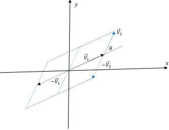
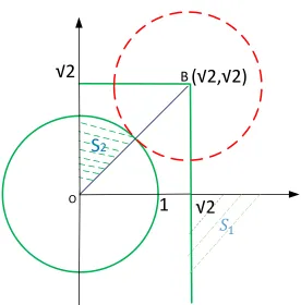
To find the value of 𝐾(2) , it will be useful to analyze the parallelogram formed by four vertices centered at the origin, resulting from the four combinations ∓𝑉,⃗: ∓ 𝑉,⃗Q (see Figure1)

By using the cosine rule, we can find the length of the big and the small diagonals respectively as follows:

ž𝐿 Q _{= 7𝑉,⃗}

:7_Q+ 7𝑉,⃗Q7_Q+ 27𝑉,⃗:7_Q7𝑉,⃗Q7_Qcos (𝜃) 𝑙Q_{= 7𝑉,⃗}

:7_Q+ 7𝑉,⃗Q7_Q− 27𝑉,⃗:7_Q7𝑉,⃗Q7_Qcos(𝜃) , −𝑉,⃗_:

𝑉,⃗_:

−𝑉,⃗_Q 𝑉,⃗Q

𝜃

𝑥 𝑦

5 where 𝜃 is the acute angle between the two vectors 𝑉,⃗: and 𝑉,⃗Q .

We can notice that the small diagonal 𝑙 has √2 as an upper bound, i.e.,

Œ7𝑉,⃗_:7_Q+ 7𝑉,⃗_Q7_Q− 27𝑉,⃗_:7_Q7𝑉,⃗Q7_Qcos(𝜃) ≤ Œ7𝑉,⃗:7_Q+ 7𝑉,⃗Q7_Q≤ √2 .

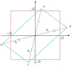
As it was mentioned before, the two weights, 𝜀: and 𝜀Q , can be chosen in such a way the length of 𝜀:𝑉,⃗:+ 𝜀Q𝑉,⃗Q is smaller than the length of diagonal 𝑙, in which it implies that for all vectors 𝑉,⃗E inside the circle of center (0,0) and Radius =1, we can find 𝜀: and 𝜀Q such that 7𝜀:𝑉,⃗:+ 𝜀Q𝑉,⃗Q 7_J ≤ 𝐾(𝑛) ≤ √2 . In different method the prove of 𝐾(2) ≤ √2 can be carried out by using technic of proof by

contradiction. Let’s assume the case where the vertices A, B, C, and D are located outside of the red square of side 2√2 as it is shown in Figure 2.

The possibility of having all vertices,∓𝑉,⃗: ∓ 𝑉,⃗Q , outside the red square in Figure 2 is impossible! Because it contradicts with the fact that small diagonal length is at less or eqal t0 √2.

From previous proof, we can conclude that 𝐾(2) ≤ √2, and it is enough to find a particular case where min

@” 7𝜀:𝑉,⃗:+ 𝜀Q𝑉,⃗Q 7J = √2 in order to prove that 𝐾(2) = √2.

√2 √2

−√2

−√2 𝑑Q

𝑑_S

𝑑U

𝐵 𝐴

𝐶 𝐷

Figure 2. ABCD is a parallelogram with for vertices located outside of square whose side is √2 ℎ𝑎𝑠 𝑚𝑖𝑛

6 Lt’s considerthe case where 𝑉,⃗:=_√Q: §+1₊₁¨ and 𝑉,⃗Q=_√Q: §−1₊₁¨ , so for any possible values of 𝜀: and 𝜀Q , we can calculate the value min

@” 7𝜀:𝑉,⃗:+ 𝜀Q𝑉,⃗Q 7Jas follows: max „|𝜀:+ 𝜀|

√2 ,

|𝜀:− 𝜀Q|

√2 … = max ©

ª1 + 𝜀Q _𝜀 : « ª

√2 ,

ª1 − 𝜀Q _𝜀 : « ª

√2 ¬

= 1

√2 max •1 + ª𝜀 Q _𝜀

:

« ª , 1 − ª𝜀Q _𝜀 : « ª•

= 2 √2 . Therefore, we can conclude that 𝐾(2) = √2.

Evaluation of

𝑲(𝟑)

:

Given the vector space ℝS_{, the span of the set 𝑆 of finite vectors is defined as the set of all linear} combinations of the vectors in 𝑆, noted as follows:

𝑆𝑝𝑎𝑛(𝑆) = žm 𝛼E𝑉,⃗E p

EI:

; 𝑘 ∈ ℕ , 𝑉,⃗E∈ 𝑆, 𝛼E ∈ ℝ ³ .

The calculation of 𝐾(3) will be splited to several cases related to different configurations of the three vectors 𝑉,⃗:, 𝑉,⃗Q, and 𝑉,⃗S in ℝS.

Case 1: 𝑉,⃗S ⊥ 𝑆𝑝𝑎𝑛•𝑉,⃗Q, 𝑉,⃗:• and 𝑆𝑝𝑎𝑛•𝑉,⃗Q, 𝑉,⃗:• = 𝑥-𝑦 plane.

As the vector 𝑉,⃗S is parallel to 𝑦-axe, then without losing generality, we can write the following: min

@” 7𝜀⃗S𝑉,⃗S+ 𝜀⃗Q𝑉,⃗Q+ 𝜀⃗:𝑉,⃗: 7J=min@” 7𝑉,⃗S+ 𝜀⃗Q𝑉,⃗Q+ 𝜀⃗:𝑉,⃗: 7J by consequence,

min

@” 7𝑉,⃗S+ 𝜀⃗Q𝑉,⃗Q+ 𝜀⃗:𝑉,⃗: 7J=𝑚𝑎𝑥 µ7𝑉,⃗S 7

Q, min@” 7𝜀⃗Q𝑉,⃗Q+ 𝜀⃗:𝑉,⃗: 7J ¶.

From previous section, we know that the constant 𝐾(2) = √2 and from the fact that 𝜀⃗Q𝑉,⃗Q+ 𝜀⃗:𝑉,⃗:∈ 𝑥-𝑦 plane, we have

𝑚𝑎𝑥 µ7𝑉,⃗S7_Q, min_@

” 7𝜀⃗Q𝑉,⃗Q+ 𝜀⃗:𝑉,⃗: 7J ¶ ≤ 𝑚𝑎𝑥 37𝑉,⃗S 7

Q, √2 ; ≤ √2.

By considering 𝑉,⃗:=_√Q: © +1 +1 0

¬ , 𝑉,⃗Q=_√Q: © −1 +1 0

¬ , and 𝑉,⃗S= © 0 0 +1

7 lm 𝜀E 𝑉,⃗E

S

EI: l

J

= max „|𝜀:+ 𝜀Q| √2 ,

|𝜀:− 𝜀Q|

√2 , |𝜀S|…

= max „|1 + 𝜀Q| √2 ,

|1 − 𝜀_Q| √2 ,1… = √2.

Therefore, under the case 1, the value 𝐾(3) is equal to √2 . Case 2: 𝑆𝑝𝑎𝑛•𝑉,⃗:, 𝑉,⃗Q• = 𝑥-𝑦 plane.

We split the vector 𝑉,⃗S as follows:

𝑉,⃗S= 𝑉,⃗S:⨁𝑉,⃗SQ , where 𝑉,⃗S: ⊥ XY-plane. Without losing generality, the value of the weight 𝜀S can be fixed to 1 in our calculation.

Therefore, for all vectors 𝑉,,,⃗ , 𝑉: ,,,⃗, 𝑉Q ,,,⃗ ∈ ℝS S with 7𝑉,,⃗ 7G _Q≤ 1

min

@” lm 𝜀E𝑉,⃗E S

EI: l

J

= min

@” l𝑉,⃗S+ m 𝜀E𝑉,⃗E Q

EI: l

J

= max ¸7𝑉,⃗_S:7_Q, min

@” l𝑉,⃗SQ+ m 𝜀E𝑉,⃗E Q

EI: l

J ¹

From previous equation, we can see that the calculation is moved from dimension 3 to dimension 2 by just calculating the following:

For all vectors 𝑉,,,⃗ , 𝑉: ,,,⃗, 𝑉Q ,,,,,,⃗ ∈ ℝSQ Q with 7𝑉,,⃗ 7G _Q≤ 1, the below maximum is needed to be calculated

max *º

,,,⃗ ∈ℝ»_{∶ 7*,,,⃗ 7º} 89:

min

@” l𝑉,⃗SQ+ m 𝜀E𝑉,⃗E Q

EI: l

J

where 𝑉,⃗SQ= „ 𝛼 𝛽

0…, and without losing generality, the two assumption 𝛼

Q_{+ 𝛽}Q _{≤ 1 and 0 ≤ 𝛼 ≤ 𝛽 ≤ 1}

can be added.

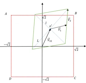
8 From the Figure 4, the small diagonal, 𝑙, of parallelogram centered at the point 𝑂′ is at most equal to √2 , consequently, we have to focus only on the green area, highlighted in Figure 5, the possible location of two opposite vertices that form the two small diagonal 𝑙.

√2 √2

−√2

−√2 𝐴

𝐷 𝐶

𝐵

𝑉,⃗_:

𝐿 𝑙

𝑉,⃗SQ

𝑉,⃗Q 𝑜′

Figure 3 Without losing generality, the vector 𝑉,⃗_SQ can be consider with slope bigger than one, 𝑚 ≥1. The two distances 𝑙

9 Figure 4 Green Area is the only possible location of the vertices,𝑉,,,,,,⃗ ∓ 𝑉SQ ,,,⃗ ∓ 𝑉: ,,,⃗Q , in order to have maybe

7𝑉,,,,,,⃗ ∓ 𝑉SQ ,,,⃗ ∓ 𝑉: ,,,⃗7Q _J > √2

The distance between the point 𝑂¿ _{and the midpoint of any two adjacent vertices is equals to either} 7𝑉,⃗:7 or 7𝑉,⃗Q7 , which implies that the impossibility to have, on one side of square, two vertices outside of square, refer to Figure 4.

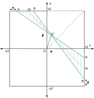
This impossibility can be proved by highlighting the fact that the distance between any point inside the area 𝑆: and any point inside the area 𝑆Q is bigger than or equal to 1, see Figure 5.

x y

-√2

α _{A A1}

A’

A0

β

B’ B

O’

O √2

-√2

10 Figure 5. Distance between any point in the area S1 and any point in the area S2 has minimum distance of 1,

𝑆:= )𝑥 ≥ √2 𝑎𝑛𝑑 𝑦 ≤ 01 and 𝑆Q= {𝑥Q+ 𝑦Q≤ 1 𝑎𝑛𝑑 0 ≤ 𝑥 ≤ 𝑦 ≤ 1}, where the red and green circles have radius of 1 and centred at the point B and O respectively.

Therefore, under the case 2, the constant 𝐾(3) is upper bounded by √2 .

To conclude that 𝐾(3) = √2, it is enough to check the function 𝐾(3) for 𝑉,⃗:=_√Q: © +1 +1

0 ¬ , 𝑉,⃗Q = :

√Q© −1 +1

0 ¬ , and 𝑉,⃗S =_√Q: ©

0 0

+1¬, where

min

@” lm 𝜀E𝑉,⃗E S

EI: l

J

= √2.

Case 3: General case

By symmetry, without losing generality, we can consider the weight 𝜀S = 1 in our calculations, as it is proven below

√

2

√

2

₍

_√

_2,

_√

₂₎

S

2

1

𝑆

B

11 min

@” lm 𝜀E𝑉,⃗E S

EI: l

J

= min

@” l𝜀Sm 𝜀E 𝜀_S𝑉,⃗E S

EI: l

J

= min @” l𝑉,⃗S

+ m𝜀E 𝜀S𝑉,⃗E Q

EI: l

J

= min

@À Á𝑉,⃗S+ m 𝜀Â𝑉,⃗E Q

ÂI: Á

J .

The vector ∑QEI:𝜀E𝑉,⃗E will be evaluated over two perpendicular spaces, 𝑥-𝑦 plane and 𝑧 -axe, and a link between the two space will be found in order to maximize the 7∑SEI:𝜀E𝑉,⃗E7_J.

The projection of the vector 𝑉,⃗E over the space 𝑥-𝑦 plane, 𝑃𝑟𝑜𝑗 ÆÇBÈÉÊH•𝑉,⃗E•, is denoted by vector 𝑈,,⃗E. From case 2 , we have proven that it is not possible to have all vertices, 𝑈,,⃗S± 𝑈,,⃗Q± 𝑈,,⃗:, outside the square of side 2√2 centered at the origin. An important question rises about the possibility to increase the 𝑙J norm beyond √2 for two vertices and compensate the 𝑙J norms of the two other vertices by 𝑙J norm over 𝑧-axe?

To answer the previous question, we need to find 𝑧-coordinates of three vectors 𝑉,⃗E that satisfy the following statement:

For each possible weight’s vector (1, 𝜀:, 𝜀Q) where 7𝑈,,⃗S+ ∑QÂI:𝜀Â𝑈,,⃗E7_J < √2 then 7𝑍S+ ∑QÂI:𝜀Â𝑍E7_J= ª𝑍S+ ∑QÂI:𝜀Â𝑍Eª > √2 .

To summarize the above idea, we create an example of vectors 𝑉,⃗E, where 7∑SEI:𝜀E𝑉,⃗E7_J> √2, as follows:

𝑉,⃗_:= © −𝑥_:

𝑦_:

𝑧_: ¬ , 𝑉,⃗Q= © −𝑥_Q

𝑦_Q

−𝑧_Q¬ , and 𝑉,⃗S= © 𝑥_S 𝑦_S 𝑧_S¬, where 𝑥E , 𝑦E, 𝑧E are all non-negative value with 7𝑉,⃗E7_Q= X𝑥EQ+ 𝑦EQ+ 𝑧EQ≤ 1 , We assume the following equations

𝑖𝑓 ž7𝑉,⃗S− 𝑉,⃗Q− 𝑉,⃗:7J = 𝑥:+ 𝑥Q+ 𝑥S = 𝐾: 7𝑉,⃗S+ 𝑉,⃗Q+ 𝑉,⃗:7_J= 𝑦:+ 𝑦Q+ 𝑦S= 𝐾Q

𝑡ℎ𝑒𝑛 ž 7𝑉,⃗S− 𝑉,⃗Q+ 𝑉,⃗:7J= 𝑧:+ 𝑧Q+ 𝑧S= 𝐾S 7𝑉,⃗S+ 𝑉,⃗Q− 𝑉,⃗:7_J = |𝑧S− 𝑧:− 𝑧Q| = 𝐾U.

12 Then the system that is needed to be solved is summarized by the following equations:

Î

𝑥_:+ 𝑥_Q+ 𝑥_S = 𝐾_: 𝑦:+ 𝑦Q+ 𝑦S= 𝐾: 𝑧_:+ 𝑧_Q+ 𝑧_S= 𝐾_S 𝑧_:+ 𝑧_Q− 𝑧_S= 𝐾_S

From the last two equations, we conclude that

𝑧_S= 0 By symmetry, we can conclude that

𝑥_S= 𝑦_S

Since 7𝑉,⃗S7 ≤ 1 , it is convenient to increase 𝑥S& 𝑦S as much as we can in order to maximum the value of 𝐾:, where it can be found when the coordinates of 𝑉,⃗S are :

𝑥_S= 𝑦_S= 1 √2 Therefore, the system will be simplified again as follows

⎩ ⎪ ⎨ ⎪

⎧𝑥:+ 𝑥Q= 𝐾:−√2₂

𝑦_:+ 𝑦_Q = 𝐾_:−√2 2 𝑧_:+ 𝑧_Q= 𝐾_S Again by symmetry, we can consider the following equations:

𝑥_:= 𝑦_:= 𝛼 𝑥_Q= 𝑦_Q= 𝛽 𝑧:= 𝑧Q = 𝛾

In order to maximize 𝐾 and by symmetry, we need to impose that 𝐾: = 𝐾S, then the final system that need to be solved is as follows:

⎩ ⎪ ⎨ ⎪

⎧ 𝛼 + 𝛽 = 𝐾 −√2 2 𝛾 = 𝐾

2 𝛼Q_{+ 𝛽}Q_{+ 𝛾}Q_{≤ 1 ,}

13 The maximum value of 𝐾 can be calculated by

⎩ ⎪ ⎨ ⎪

⎧ 𝛼 = 𝐾 2 −

√2 4 𝛾 = 𝐾

2 2𝛼Q_{+ 𝛾}Q _{= 1}

So, we end up to solve the below quadratic equation

2 „𝐾 2 −

√2 4…

Q + <𝐾

2 K Q

= 1

After simplification, we find:

3𝐾Q_{− 2√2𝐾 − 3 = 0}

The solution of previous quadratic equation is when the value 𝐾 is equal to √QR√::_S . Hence

𝐾(3) ≥√QR√:: S .

A simulation is used to answer the question if the value 𝐾(3) is eqal to √QR√::_S or not. A cylindrical Coordinate has been used in our simulation to check most of the cases, the possible coordinate’s values of the vector 𝑉,⃗E are summarized as follows:

𝑥 = 𝑟 𝑐𝑜𝑠(𝜃)sin (𝛼) 𝑦 = 𝑟 𝑠𝑖𝑛(𝜃)sin (𝛼)

𝑧 = 𝑟 𝑐𝑜𝑠 (𝛼)

where 𝜃 = [𝑠𝑡𝑎𝑟𝑡 𝑣𝑎𝑙𝑢𝑒: 𝑠𝑡𝑒𝑝: 𝑒𝑛𝑑 𝑣𝑎𝑙𝑢𝑒] = [0: 0.001: 2𝜋] , 𝛼 = [𝑠𝑡𝑎𝑟𝑡 𝑣𝑎𝑙𝑢𝑒: 𝑠𝑡𝑒𝑝: 𝑒𝑛𝑑 𝑣𝑎𝑙𝑢𝑒] = [0: 0.001: 2𝜋] , and 𝑟 = [𝑠𝑡𝑎𝑟𝑡 𝑣𝑎𝑙𝑢𝑒: 𝑠𝑡𝑒𝑝: 𝑒𝑛𝑑 𝑣𝑎𝑙𝑢𝑒] = [0: 0.01: 1].

The simulation has showed that the value 𝐾(3) is equl to √QR√::_S i.e. 𝐾(3) =√QR√::_S .

The constant

𝑲(𝟒)

Before giving the approach for dimension 4, we will review the evaluation 𝐾(3) for dimension 2 and 3 in a different ways in order to be generalized later on.

For dimension 2, we denote by 𝑉,⃗:= § 𝛼_:

𝛽:¨ and 𝑉,⃗Q= § 𝛼_Q

14 min

@+ 7𝑉,⃗:+ 𝜀Q𝑉,⃗Q7J= 𝐾(2). By symmetry, we can assume that

7𝑉,⃗:+ 𝑉,⃗Q7_J= 𝛼:+ 𝛼Q= 𝐾(2)

7𝑉,⃗:− 𝑉,⃗Q7_J= 𝛽:− 𝛽Q= 𝐾(2)

From the definition of 𝐾(2), to get the maximum value of it, the coordinates of the two vectors should be non-negatives values except the coordinate 𝛽Q should be a negative value.

By symmetry, we denote 𝛼:= 𝛼Q= 𝛼 & 𝛽:= −𝛽Q= 𝛽 . to find 𝐾(2), it is a enough to solve the following system:

µ2𝛼 = 𝐾(2)_{2𝛽 = 𝐾(2)}

under the constraint 𝛼Q_{+ 𝛽}Q_{≤ 1 .}

The maximum 𝐾(2) can be found by considering 𝛼Q_{+ 𝛽}Q_{= 1 , so the previous system is equivalent to} the following quadratic equation

<𝐾(2) 2 K

Q

+ <𝐾(2) 2 K

Q = 1

Therefore

𝐾(2) = √2.

For dimension 3 , we would like to find 𝑉,⃗:= © 𝛼: 𝛽:

𝛾_:¬ , 𝑉,⃗Q= © 𝛼Q 𝛽Q

𝛾_Q¬ and 𝑉,⃗S= © 𝛼S 𝛽S

𝛾_S¬ that verify 𝐾(3) = min

@+,@87𝑉,⃗S+ 𝜀Q𝑉,⃗Q+ 𝜀:𝑉,⃗:7J.

All possible cases of the vector 𝜀⃗ = „ 𝜀_: 𝜀Q

1… will be gathered under a matrix named 𝐴S, where its rows 𝑟E form all cases of the vector 𝜀⃗ .

The matric 𝐴S is defined as follows:

𝐴_S= Ý

+1 +1 +1 +1 −1 +1 +1 +1 −1 +1 −1 −1

Þ.

15 7𝑉,⃗S+ 𝑉,⃗Q+ 𝑉,⃗:7_J= |𝛼S+ 𝛼Q+ 𝛼:| = 𝐾(3)

7𝑉,⃗S+ 𝑉,⃗Q− 𝑉,⃗:7_J= |𝛽S+ 𝛽Q− 𝛽:| = 𝐾(3)

7𝑉,⃗S− 𝑉,⃗Q+ 𝑉,⃗:7_J = |𝛾S− 𝛾Q+ 𝛾:| = 𝐾(3)

7𝑉,⃗S− 𝑉,⃗Q− 𝑉,⃗:7_J = |𝛾S− 𝛾Q− 𝛾:| = 𝐾(3)

In order to maximize the value of 𝐾(3) , it is suitable to consider the coordinates 𝛽:, 𝛾:, and 𝛾Q as a negative values, so the coordinate of the three vectors 𝑉,⃗E will be summarized as following

𝑉,⃗:= ©− 𝛼_: 𝛽:

−𝛾_:¬ , 𝑉,⃗Q= © 𝛼_Q 𝛽Q

−𝛾_Q¬ and 𝑉,⃗S= © 𝛼_S 𝛽S 𝛾_S¬, where all parameters, (𝛼E , 𝛽E , 𝛾E) are non-negative values.

To calculate 𝐾(3) , it is enough to solve the below system:

Î

𝛼S+ 𝛼Q+ 𝛼:= 𝐾(3) 𝛽_S+ 𝛽_Q+ 𝛽_:= 𝐾(3) 𝛾_S+ 𝛾_Q+ 𝛾_:= 𝐾(3) −𝛾S+ 𝛾Q+ 𝛾:= 𝐾(3) Under the constraints

𝛼_:Q_{+ 𝛽}

:Q+ 𝛾:Q≤ 1 𝛼_QQ_{+ 𝛽}

QQ+ 𝛾QQ≤ 1 𝛼SQ+ 𝛽SQ+ 𝛾SQ≤ 1

From the last two equations of the system we can conclude that 𝛾S = 0 . By symmetry also, we can assume that

𝛼:= 𝛼Q= 𝛽Q= 𝛽:= 𝛽 𝛾Q= 𝛾:= 𝛾 𝛼_S= 𝛽_S= 𝛼 Therefore,

µ2𝛽 + 𝛼 = 𝐾(3)_{2𝛾 = 𝐾(3)}

Under the constraints

16 In order to maximize the value of 𝐾(3), the two constraints can be considered as

2𝛽Q_{+ 𝛼}Q_{= 1} 2𝛼 = 1 Then the system will be simplified as follows

¸2𝛽 = 𝐾(3) −√2₂ 2𝛾 = 𝐾(3)

The below quadratic equation is needed to be solved to calculate the value 𝐾(3) , 2 §ß(S)_Q −√Q_U¨Q+ §ß(S)_Q ¨Q= 1 .

After simplification, the quadratric equation can be as follows: 3𝐾(3)Q_{− 2√2𝐾(3) − 3 = 0}

As a consequence, it concludes that

𝐾(3) =√2 + √11

3 .

The particular vectors that cannot canceled each other further than 𝐾(3) are define as follows:

𝑉,⃗:= ⎝ ⎜ ⎛ ß(S) U − √Q U Bß(S) U + √Q U −ß(S) Q ⎠ ⎟ ⎞

, 𝑉,⃗Q= ⎝ ⎜ ⎛ ß(S) U − √Q U ß(S) U − √Q U −ß(S) Q ⎠ ⎟ ⎞

and 𝑉,⃗S= ⎝ ⎛ √Q Q √Q Q 0 ⎠ ⎞_.

Note that these particular three vectors are not unique solution of arg_*,,⃗”min @” 7∑ 𝜀E𝑉,⃗E

7 J.

The idea is to generalize the previous approach in evaluating the function 𝐾(𝑛), for that let’s denote by 𝑉 = {𝑉,⃗_U, 𝑉,⃗S, 𝑉,⃗Q, 𝑉,⃗:} the set of particular vectors that satisfy the below equation

𝐾(4) = min

@+,@8,@»l𝑉,⃗U+ m 𝜀E𝑉,⃗E S

EI: l

J .

17 𝐴_U=

⎣ ⎢ ⎢ ⎢ ⎢ ⎢ ⎢

⎡+1 +1 +1 +1_{+1 −1 +1 +1} +1 +1 −1 +1 +1 −1 −1 +1 +1 +1 +1 −1 +1 −1 +1 −1 +1 +1 −1 −1 +1 −1 −1 −1⎦

⎥ ⎥ ⎥ ⎥ ⎥ ⎥ ⎤

,

where it is noted that 𝑟ERQ = 𝑟ER:+ 𝑟E− 𝑟EB: , for 𝑖 > 1, and dim•𝑠𝑝𝑎𝑛(𝑟:, 𝑟Q, 𝑟S)• = 3.

The idea is to well assign each row 𝑟E to one of fourth dimension in order to avoid zero coordinate in 𝑉,⃗E , which it is a consequence of maximizing the value of 𝐾(4), i.e., the axes where 𝑙J norm of 𝑉,⃗U+ ∑SEI:𝜀E𝑉,⃗E is located will be distributed over all possible combinations of (1, 𝜀:, 𝜀Q, 𝜀S) in a way to maximize the value 𝐾(4).

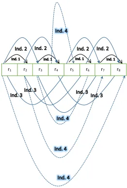
The below diagram, in Figure 6, identifies which coordinate will be eliminated, being zero, when we associate two rows to same axes.

r1 r2 r3 r4 r5 r6 r7 r8

f h f h f h f h

18 From previous diagram, the rows are gathered as follows

• (𝑟_:, 𝑟Q): 7𝑉,⃗U± 𝑉,⃗S+ 𝑉,⃗Q+ 𝑉,⃗:7_J= ª𝑉U:± 𝑉S:+ 𝑉Q:+ 𝑉::ª = 𝐾(4) • (𝑟í, 𝑟î): 7𝑉,⃗U+ 𝑉,⃗S± 𝑉,⃗Q− 𝑉,⃗:7_J = ª𝑉UQ+ 𝑉SQ± 𝑉QQ− 𝑉:Qª = 𝐾(4) • (𝑟_U, 𝑟_ï): 7𝑉,⃗_U− 𝑉,⃗_S− 𝑉,⃗_Q± 𝑉,⃗_:7_J= ª𝑉_US_{− 𝑉}

SS− 𝑉QS± 𝑉:Sª = 𝐾(4) • (𝑟_S, 𝑟_ð): 7±𝑉,⃗_U+ 𝑉,⃗_S− 𝑉,⃗_Q+ 𝑉,⃗_:7_J= |±𝑉_UU_{+ 𝑉}

SU− 𝑉QU+ 𝑉:U|= 𝐾(4), where 𝑉_EÂ is the jth _{coordinate of vector 𝑉,⃗}

E.

In order tomaximize the value 𝐾(4), the coordinate’s sign of 𝑉,⃗E can be found as follows:

𝑉,⃗_:= ñ 𝛼_: −𝛽_Q

𝛾Q 𝑤_Q

ò , 𝑉,⃗Q= ñ 𝛼_Q 𝛽_Q −𝛾Q −𝑤_Q

ò , 𝑉,⃗S= ñ 𝛼_S 𝛽S −𝛾S

𝑤_U

ò and 𝑉,⃗U= ñ 𝛼_U 𝛽_U 𝛾U 𝑤_U

ò,

where 𝛼E , 𝛽E , 𝛾E and 𝑤E are non-negative values.

The negative sign highlighted at the coordinate of 𝑉,,⃗G comes from rows 𝑟:, 𝑟í, 𝑟U, 𝑎𝑛𝑑 𝑟S. For instance, if we assume that 7𝑉,⃗U+ ∑SEI:𝜀E𝑉,⃗E7_J= ª∑SEI:𝜀E𝛼E+ 𝛼Uª, where 𝑟U= (1, −1, −1,1), in order to get maximum value of 𝐾(4), it is preferable to consider the two coordinates 𝛼Q and 𝛼S as negative values such that the equation 1(𝛼:) − 1(𝛼Q) − 1(𝛼S) + 1(𝛼U) = 𝐾(4) will be equivalent to the equation

|𝛼_:| + |𝛼_Q| + |𝛼_S| + |𝛼_U| = 𝐾(4). The rows distribution can formulated by the following systems of equations

(𝑟_:, 𝑟_Q): µ𝛼U+ 𝛼S+ 𝛼Q+ 𝛼:= 𝐾

𝛼_U− 𝛼_S+ 𝛼_Q+ 𝛼_:= 𝐾 ⟹ 𝛼S= 0

(𝑟_í, 𝑟_î): µ𝛽U+ 𝛽S+ 𝛽Q+ 𝛽:= 𝐾

𝛽_U+ 𝛽_S− 𝛽_Q+ 𝛽_:= 𝐾 ⟹ 𝛽Q= 0

(𝑟_U, 𝑟_ï): µ𝛾U+ 𝛾S+ 𝛾Q+ 𝛾:= 𝐾

𝛾_U+ 𝛾_S+ 𝛾_Q− 𝛾_:= 𝐾 ⟹ 𝛾:= 0

(𝑟_S, 𝑟_ð): µ 𝑤U+ 𝑤S+ 𝑤Q+ 𝑤:= 𝐾

−𝑤_U+ 𝑤_S+ 𝑤_Q+ 𝑤_:= 𝐾 ⟹ 𝑤U= 0

19 Î

𝛼_U+ 𝛼_Q+ 𝛼_:= 𝐾 𝛽U+ 𝛽S+ 𝛽:= 𝐾 𝛾_U+ 𝛾_S+ 𝛾_Q= 𝐾 𝑤S+ 𝑤Q+ 𝑤:= 𝐾

Under the below constraints

⎩ ⎪ ⎨ ⎪

⎧𝛼UQ+ 𝛽UQ+ 𝛾UQ = 1 𝑤_UQ_{+ 𝛽}

SQ+ 𝛾SQ= 1 𝛼_QQ_{+ 𝑤}

QQ+ 𝛾QQ= 1 𝛼_:Q_{+ 𝛽}

:Q+ 𝑤:Q = 1

As before, the previous system of equations needs to be matched with coordinates of the four vectors in order to maximize the value of 𝐾(4), then

ô𝑉,⃗:, 𝑉,⃗Q, 𝑉,⃗S, 𝑉,⃗Sõ = ö

𝛼_: 𝛼_Q −𝛽: 0

0 𝛼_U 𝛽_S 𝛽_U 0 −𝛾_Q

𝑤_: −𝑤_Q

−𝛾_S 𝛾_U 𝑤_S 0

÷.

By symmetry, we can assume that

𝛼U= 𝛼Q= 𝛼:= 𝛼 𝛽_U= 𝛽_S= 𝛽_:= 𝛽 𝛾U= 𝛾S= 𝛾Q = 𝛾 𝑤_S= 𝑤_Q = 𝑤_:= 𝑤 Therefore

Î

𝛼 = 𝐾/3 𝛽 = 𝐾/3 𝛾 = 𝐾/3 𝑤 = 𝐾/3

To maximize 𝐾, the constraints can be assumed to be as follows: 1 = 𝛼Q_{+ 𝛽}Q_{+ 𝛾}Q = 𝛼Q_{+ 𝛽}Q_{+ 𝑤}Q = 𝛼Q_{+ 𝑤}Q_{+ 𝛾}Q = 𝑤Q_{+ 𝛽}Q_{+ 𝛾}Q

To find the value of 𝐾(4), it is enough to solve the below quadrature equation

𝛼Q_{+ 𝛽}Q_{+ 𝛾}Q _{= 3 <}𝐾 3K

20 It implies that

𝐾(4) ≥ X3,

and the coordinates of the particular set of vectors 𝑉,,⃗G are summarized under the below matrix

ô𝑉,,,⃗ 𝑉_: ,,,⃗ 𝑉Q ,,,,⃗ 𝑉,⃗S Uõ = 1 √3ö

1 1 0 1

−1 0 1 1

0 −1 −1 1

1 −1 1 0

÷.

Note: Other distribution can formulated by the following the below configuration:

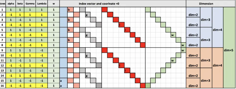
The matrix can be formulated differently as follows:

𝐴U=

⎣ ⎢ ⎢ ⎢ ⎢ ⎢ ⎢

⎡+1 +1 +1 +1_{−1 +1 +1 +1} +1 −1 +1 +1 −1 −1 +1 +1 +1 +1 −1 +1 −1 +1 −1 +1 +1 −1 −1 +1 −1 −1 −1 +1⎦

⎥ ⎥ ⎥ ⎥ ⎥ ⎥ ⎤

,

From the below Table 1, the row distribution can configurated by the following systems of equations (𝑟:, 𝑟Q): µ_−𝛼𝛼:+ 𝛼Q+ 𝛼S+ 𝛼U = 𝐾

:+ 𝛼Q+ 𝛼S+ 𝛼U= 𝐾 ⟹ 𝛼:= 0 (𝑟_ð, 𝑟ï): µ𝛽_𝛽:+ 𝛽Q+ 𝛽S+ 𝛽U= 𝐾

:− 𝛽Q+ 𝛽S+ 𝛽U= 𝐾 ⟹ 𝛽Q= 0 (𝑟_S, 𝑟_î): µ𝛾:+ 𝛾Q+ 𝛾S+ 𝛾U= 𝐾

𝛾_:+ 𝛾_Q− 𝛾_S+ 𝛾_U= 𝐾 ⟹ 𝛾S = 0

(𝑟_U, 𝑟_í): µ𝑤:+ 𝑤Q+ 𝑤S+ 𝑤U= 𝐾

21 Table 1 How to gather two rows of the matrix in order to eliminate a given index coordinate.

By finishing the calculation, we find that

𝐾(4) ≥ √3.

The Cauchy-Schwarz inequality, also known as the Cauchy–Bunyakovsky–Schwarz inequality, can be used to optimized the following system:

Maximizing the variable 𝐾, under the fourth objective functions:

Î

𝛼Q+ 𝛼S+ 𝛼U= 𝐾 𝛽:+ 𝛽S+ 𝛽U= 𝐾 𝛾:+ 𝛾Q+ 𝛾U = 𝐾 𝑤_:+ 𝑤_Q+ 𝑤_S= 𝐾

Under the below constraints:

⎩ ⎪ ⎨ ⎪

⎧𝛼UQ+ 𝛽UQ+ 𝛾UQ = 1 𝑤_SQ_{+ 𝛽}

SQ+ 𝛾SQ= 1 𝛼_QQ_{+ 𝑤}

QQ+ 𝛾QQ= 1 𝛾_:Q_{+ 𝛽}

:Q+ 𝑤:Q= 1

The system can be modified by Cauchy as follows:

⎩ ⎪ ⎨ ⎪

⎧ 𝐾Q = (𝛼Q+ 𝛼S+ 𝛼U) Q≤ (𝛼QQ+ 𝛼SQ+ 𝛼UQ)(1Q+ 1Q+ 1Q) 𝐾Q _{= (𝛽}

:+ 𝛽S+ 𝛽U) Q≤ (𝛽:Q+ 𝛽SQ+ 𝛽UQ)(1Q+ 1Q+ 1Q) 𝐾Q_{= (𝛾}

:+ 𝛾Q+ 𝛾U) Q≤ (𝛾:Q+ 𝛾QQ+ 𝛾UQ)(1Q+ 1Q+ 1Q) 𝐾Q_{= (𝑤}

:+ 𝑤Q+ 𝑤S) Q≤ (𝑤:Q+ 𝑤QQ+ 𝑤SQ)(1Q+ 1Q+ 1Q)

By adding all the four equation will get 4𝐾Q_{≤ 3(𝛼}

U Q_{+ 𝛼}

QQ+ 𝛼SQ+ 𝛽UQ+ 𝛽SQ+ 𝛽:Q+ 𝛾UQ+ 𝛾QQ+ 𝛾:Q+ 𝑤SQ+ 𝑤QQ+ 𝑤:Q), from constraints, the maximum of the value 𝐾 can be calculated as follows:

4𝐾Q_{= 12,} then the constant of the optimization is found to be as follows

𝐾 = √3, Then the komlos constant has a lower bound as follows

22 The coordinate of the four vectors can be calculated from the equality of Cauchy-Schwarz inequality property that states that

⎩ ⎪ ⎪ ⎨ ⎪ ⎪

⎧ (𝛼U+ 𝛼Q+ 𝛼S) Q= (𝛼UQ+ 𝛼QQ+ 𝛼SQ)(1Q+ 1Q+ 1Q) ⟹ 𝛼_S

1 = 𝛼_Q

1 = 𝛼_U

1 (𝛽_U+ 𝛽_S+ 𝛽_:) Q_{= (𝛽}

UQ+ 𝛽SQ+ 𝛽:Q)(1Q+ 1Q+ 1Q) ⟹ 𝛽:

1 = 𝛽S

1 = 𝛽U

1 (𝛾_U+ 𝛾_Q+ 𝛾_:) Q_{= (𝛾}

UQ+ 𝛾:Q+ 𝛾QQ)(1Q+ 1Q+ 1Q) ⟹ 𝛾_:

1 = 𝛾_Q

1 = 𝛾_U

1 (𝑤_S+ 𝑤_Q+ 𝑤_:) Q_{= (𝑤}

SQ+ 𝑤QQ+ 𝑤:Q)(1Q+ 1Q+ 1Q) ⟹ 𝑤:

1 = 𝑤Q

1 = 𝑤S

1

Therefore

𝛼_E = 𝛽_E= 𝛾_E = 𝑤_E =√3 3 .

The coordinate of the particular vectors 𝑉,,⃗G are summarized under the below matrix

ô𝑉,,,⃗ 𝑉: ,,,⃗ 𝑉Q ,,,⃗ 𝑉S ,,,⃗õ =U √3

3 Ý

0 +1

+1 0 +1 +1−1 +1 +1 −1

−1 −1 +1 0 0 +1 Þ.

In the case where the dimension is under the form of 2ø_{, for certain integer m, the optimization is} perfect but for other cases of dimension an upper bound can be found for the constant K if Cauchy-Schwarz inequality is applied as above.

Evaluation of

𝑲(𝟓)

By using the same idea of the previous section, in dimension 4, we denote by 𝑉,,,⃗, … , 𝑉: ,,,⃗í as a special vectors satisfying

𝐾(5) = min

@” l𝑉,⃗í+ m 𝜀E𝑉,⃗E U

EI: l

J

23 𝐴í= ⎣ ⎢ ⎢ ⎢ ⎢ ⎢ ⎢ ⎢ ⎢ ⎢ ⎢ ⎢ ⎢ ⎢ ⎢

⎡+1 +1 +1 +1 +1_{−1 +1 +1 +1 +1} +1 −1 +1 +1 +1 −1 −1 +1 +1 +1 +1 +1 −1 +1 +1 −1 +1 −1 +1 +1 +1 −1 −1 +1 +1 −1 −1 −1 +1 +1 +1 +1 +1 −1 +1 −1 +1 +1 −1 +1 +1 −1 +1 −1 +1 −1 −1 +1 −1 +1 +1 +1 −1 −1 +1 −1 +1 −1 −1 +1 +1 −1 −1 −1 +1 −1 −1 −1 −1 +1⎦

⎥ ⎥ ⎥ ⎥ ⎥ ⎥ ⎥ ⎥ ⎥ ⎥ ⎥ ⎥ ⎥ ⎥ ⎤

where it is noted that 𝑟ERQ = 𝑟ER:+ 𝑟E− 𝑟EB: , for 𝑖 > 1 and 𝑑𝑖𝑚{𝑟E, 𝑖 = 1, … ,16} = 5.

The target is to distribute the 16 rows among to five dimensions, named {∝, 𝛽, 𝛾, 𝜆, 𝑤} in such way to

minimize number of zeros in the 5 vectors, 𝑉,⃗E= ⎝ ⎜ ⎛ 𝛼_E 𝛽_E 𝛾𝑖 𝜆_E 𝑤E⎠

⎟ ⎞

, 𝑖 = 1, … ,5.

The rows distribution is summarized as following:

• Four rows will be assigned to each axe except axe 𝛼, where one row is a linear combination of the others 𝑟ERQ= 𝑟ER:+ 𝑟E− 𝑟EB:, it looks like each three independent rows will be assigned to one axe,

• Two rows will be assigned to axe 𝛼

Formulating the previous distribution of the 16 rows to the below 16 equations as follows: For 𝛼-Axe: 7𝑽,,⃗𝟓+ ∑𝟒𝒊I𝟏𝜺𝒊𝑽,,⃗𝒊7_J= ∑𝟒𝒊I𝟏|𝜺𝒊𝜶𝒊| + |𝜶𝟓|

µ𝑟_𝑟:í: 𝛼í+ 𝛼U+ 𝛼S+ 𝛼Q+ 𝛼: = 𝐾(5)

:ð: 𝛼í+ 𝛼U+ 𝛼S+ 𝛼Q− 𝛼: = 𝐾(5)⟹ 𝛼:= 0

For 𝛽-Axe: 7𝑽,,⃗_{𝟓+ ∑}𝟒 _𝜺𝒊𝑽,,⃗_𝒊

𝒊I𝟏 7_J = ∑𝟒𝒊I𝟏|𝜺𝒊𝜷𝒊| + |𝜷𝟓|

Î

𝑟_:: 𝛽_í+ 𝛽_U+ 𝛽_S+ 𝛽_Q+ 𝛽_:= 𝐾(5) 𝑟_S: 𝛽_í+ 𝛽_U+ 𝛽_S− 𝛽_Q+ 𝛽_:= 𝐾(5) 𝑟í: 𝛽í+ 𝛽U− 𝛽S+ 𝛽Q+ 𝛽:= 𝐾(5) 𝑟_î: 𝛽_í+ 𝛽_U− 𝛽_S− 𝛽_Q+ 𝛽_:= 𝐾(5)

⟹ 𝛽_Q= 𝛽_S = 0

24 For 𝛾-Axe: 7𝑽,,⃗𝟓+ ∑𝟒𝒊I𝟏𝜺𝒊𝑽,,⃗𝒊7_J= ∑𝟒𝒊I𝟏|𝜺𝒊𝜸𝒊| + | 𝜸𝟓|

Î

𝑟Q: 𝛾í+ 𝛾U+ 𝛾S+ 𝛾Q+ 𝛾: = 𝐾(5) 𝑟_ð: 𝛾_í+ 𝛾_U− 𝛾_S+ 𝛾_Q+ 𝛾_: = 𝐾(5) 𝑟_:v: 𝛾_í− 𝛾_U+ 𝛾_S+ 𝛾_Q+ 𝛾_: = 𝐾(5)

𝑟:U: 𝛾í− 𝛾U− 𝛾S+ 𝛾Q+ 𝛾:= 𝐾(5)

⟹ 𝛾_U = 𝛾_S= 0

Note that the last equations depend on the 3 first equations.

For 𝜆-Axe: 7𝑽,,⃗𝟓+ ∑𝟒𝒊I𝟏𝜺𝒊𝑽,,⃗𝒊7_J= ∑𝟒𝒊I𝟏|𝜺𝒊𝝀𝒊| + | 𝝀𝟓|

Î

𝑟_U: 𝜆_í+ 𝜆_U+ 𝜆_S+ 𝜆_Q+ 𝜆_:= 𝐾(5) 𝑟_í: 𝜆_í+ 𝜆_U− 𝜆_S− 𝜆_Q− 𝜆_:= −𝐾(5)

𝑟_:Q: 𝜆_í− 𝜆_U+ 𝜆_S+ 𝜆_Q+ 𝜆_:= 𝐾(5) 𝑟:S: 𝜆í− 𝜆U− 𝜆S− 𝜆Q− 𝜆:= 𝐾(5)

⟹ 𝜆U= 𝜆í= 0

Note that the last equations depend on the 3 first equations.

For w-Axe: 7𝑽,,⃗𝟓+ ∑𝟒𝒊I𝟏𝜺𝒊𝑽,,⃗𝒊7_J= ∑𝟒𝒊I𝟏|𝜺𝒊𝒘𝒊| + | 𝒘𝟓|

Î

𝑟_ð: 𝑤_í+ 𝑤_U+ 𝑤_S+ 𝑤_Q+ 𝑤_:= 𝐾(5) 𝑟_ï: 𝑤_í+ 𝑤_U+ 𝑤_S− 𝑤_Q+ 𝑤_:= −𝐾(5) 𝑟V: 𝑤í− 𝑤U− 𝑤S+ 𝑤Q+ − 𝑤: = 𝐾(5) 𝑟_::: 𝑤_í− 𝑤_U− 𝑤_S− 𝑤_Q− 𝑤_:= 𝐾(5)

⟹ 𝑤_í= 𝑤_Q = 0.

Note that the last equations depend on the 3 first equations.

From the previous systems of equations, we can shape our five vectors 𝑉,⃗E in order to maximize 𝐾(5) as follows

ô𝑉,,,⃗ 𝑉_: ,,,⃗ 𝑉Q ,,,,⃗ 𝑉,⃗S U 𝑉,⃗í õ =

⎣ ⎢ ⎢ ⎢

⎡ _𝛽0 −𝛼Q −𝛼S −𝛼U 𝛼í

: 0 0 𝛽U 𝛽í

−𝛾_: 𝛾_Q 0 0 𝛾_í

−𝜆_: − 𝜆_Q 𝜆_S 0 0

− 𝑤_: 0 − 𝑤_S 𝑤_U 0 ⎦⎥ ⎥ ⎥ ⎤ ,

where 𝛼E, 𝛽E , 𝛾E , 𝜆E , and 𝑤E are non-negative values.

The negative sign highlighted at the coordinate of 𝑉,,⃗G comes from rows 𝑟:í, 𝑟:, 𝑟Q, 𝑟U 𝑎𝑛𝑑 𝑟ð , for instance if we assume that 7𝑉,⃗í+ ∑UEI:𝜀E𝑉,⃗E7_J= ª∑UEI:𝜀E𝛼E+ 𝛼íª where 𝑟í= (1, −1, −1, −1,1) and our target is to maximize the value of 𝐾(5), then it is preferable to consider𝛼Q, 𝛼S, and 𝛼U are negative values such that the equation 1(𝛼:) − 1(𝛼Q) − 1(𝛼S) − 1(𝛼U) + 1(𝛼í) = 𝐾(5) will be equivalent to the below equation,

25 To calculate the constant 𝐾(5), we need to solve the below system

⎩ ⎪ ⎨ ⎪

⎧𝛼Q_𝛽+ 𝛼S+ 𝛼U+ 𝛼í= 𝐾(5) :+ 𝛽U+ 𝛽í = 𝐾(5) 𝛾:+ 𝛾Q+ 𝛾í= 𝐾(5)

𝜆_:+ 𝜆_Q+ 𝜆_S= 𝐾(5) 𝑤:+ 𝑤S+ 𝑤U= 𝐾(5) Under the constraint 7𝑉,⃗E7 ≤ 1, 𝑖 = 1, … ,5.

By symmetry, we can assume the following

𝛼í= 𝛼U= 𝛼S= 𝛼Q= 𝛼 𝛾í= 𝛾Q= 𝛾 𝜆S= 𝜆Q= 𝜆 𝑤_U= 𝑤_S = 𝑤 𝛽_:= 𝛾_: = 𝜆_:= 𝑤_: As 7𝑉,⃗:7_Q≤ 1 , we can put

𝛽_: = 𝛾_:= 𝜆_:= 𝑤_:=1 2

The system will be summarized as follow:

⎩ ⎪ ⎪ ⎪ ⎨ ⎪ ⎪ ⎪

⎧ 4𝛼 = 𝐾(5) 2𝛽 = 𝐾(5) −1

2 2𝛾 = 𝐾(5) −1 2 2𝜆 = 𝐾(5) −1 2 2𝑤 = 𝐾(5) −1 2 Under the constraints

1 = 𝛼Q_{+ 𝛽}Q_{+ 𝛾}Q = 𝛼Q_{+ 𝛽}Q_{+ 𝑤}Q = 𝛼_{= 𝛼}Q_Q+ 𝜆_{+ 𝜆}Q_Q+ 𝑤_{+ 𝛾Q}Q

The system be equivalent to quadratic equation

„𝐾(5) 4 …

Q

+ 2 „𝐾(5)

2 −

1 4…

26 So we can conclude that the value of 𝐾(5) is lower bounded by UR√:UQ_V i.e.

𝐾(5) ≥4 + √142

9 .

To see the importance of the way of distributing the rows among the axes is very important, we try to make, as an example, another configuration as follows:

⎩ ⎪ ⎨ ⎪

⎧(𝑟_(𝑟î, 𝑟ï, 𝑟V, 𝑟:v) 𝑓𝑜𝑟 𝛼 − 𝐴𝑥𝑒 Q, 𝑟S, 𝑟U) 𝑓𝑜𝑟 𝛽 − 𝐴𝑥𝑒 (𝑟:Q, 𝑟:U, 𝑟:ð) 𝑓𝑜𝑟 𝛾 − 𝐴𝑥𝑒 (𝑟_í, 𝑟_:S, 𝑟_:) 𝑓𝑜𝑟 𝜆 − 𝐴𝑥𝑒 (𝑟_ð, 𝑟_::, 𝑟_:í) 𝑓𝑜𝑟 𝑤 − 𝐴𝑥𝑒 The five vectors coordinate will be summarized under the below matrix

ô𝑉,,,⃗, 𝑉_: ,,,,,⃗ 𝑉Q, ,,,,,⃗ 𝑉,⃗S , U, 𝑉,⃗í õ =

⎣ ⎢ ⎢ ⎢

⎡ 0₀ −𝛼₀Q −𝛼_𝛽 S 𝛼U 0

S 𝛽U 𝛽í

−𝛾: 0 0 −𝛾U 𝛾í

𝜆_: 𝜆_Q 0 0 𝜆_í

−𝑤: 𝑤Q 0 𝑤U 0 ⎦

⎥ ⎥ ⎥ ⎤

The system that needs to be solved is formulated as follows: 𝛼Q+ 𝛼S+ 𝛼U= 𝐾(5)

𝛽_S+ 𝛽_U+ 𝛽_í= 𝐾(5) 𝛾:+ 𝛾U+ 𝛾í = 𝐾(5) 𝜆_:+ 𝜆_Q+ 𝜆_í = 𝐾(5) 𝑤:+ 𝑤Q+ 𝑤U= 𝐾(5) Under the constraints: 7𝑉,⃗E7_Q≤ 1.

By using this type of distribution, the symmetry of the matrix [𝑉,⃗:, … , 𝑉,⃗í] is not preserve, which it makes the system hard to be solve analytically and number of zero coordinate in the set of vectors 𝑉,,⃗G has been increased from 9 times to 10 times.

Therefore, the system that needs to be optimized is as follows: Max 𝐾(5) = 𝛼_Q+ 𝛼_S+ 𝛼_U

= 𝛽_S+ 𝛽_U+ 𝛽_í = 𝛾_:+ 𝛾_U+ 𝛾_í = 𝜆_:+ 𝜆_Q+ 𝜆_í = 𝑤_:+ 𝑤_Q+ 𝑤_U Under the constraints: 7𝑉,⃗E7_Q≤ 1.

27 Table 2 How to gather rows of the matrix in order to eliminate a certain axes-coordinates.

Evaluation of

𝑲(

𝒏

)

In dimension 𝑛, it is very crucial to find a best way to distribute all possible combinations of the vectors 𝜀⃗ = (1, 𝜀_:, … . , 𝜀_HB:) among the 𝑛 axes. We assume that we have (Q0)+

H * different combinations of the vector of 𝜀⃗ for which

l𝑉,⃗H+ m 𝜀E𝑉,⃗E HB:

EI: l

J

=+m 𝜀E𝑥E+ 𝑥H+= 𝐾(𝑛),

where 𝑥E is the coordinate of vector 𝑉,⃗E corresponding to 𝑥-Axe. The (Q0)+

H * vectors that have been assign to one axes has a dimension of order (𝑙𝑜𝑔Q§ Q0)+

H ¨ * , and as consequence, it implies that each vector 𝑉,⃗E has at most (𝑙𝑜𝑔Q§Q

0)+

H ¨ * null coordinates. To evaluate the constant 𝐾(𝑛) , it is enough to solve the below optimization equation

𝐾(𝑛) = max ‰”

⎝ ⎜ ⎛

m 𝑥E

HB,É-.8<Q 0)+

H K /

EI:

⎠ ⎟ ⎞ .

By imposing the symmetry conditions by choosing a good way of distribution, the non-null coordinate in each axes as constant values, i.e., 𝑥E = 𝑥.

Let 𝐵 a suset {1, … , 𝑛} of cardinality around 𝑛 −(𝑙𝑜𝑔_Q§Q0)+

28 m•𝑥_E•Q

Â∈0

= m(𝑥)Q Â∈0

≤ 1 ⟹ 𝑥 ≤

Œ𝑛 −,𝑙𝑜𝑔_Q<2HB:_{𝑛 K} /

𝑛 −,𝑙𝑜𝑔_Q<2HB:_{𝑛 K} / .

The lower bound of Kmolos conjecture can be calculated as follows:

𝐾(𝑛) ≥ 1𝑛 −2𝑙𝑜𝑔_Q„2HB: 𝑛 …3 ≥ Xlog(𝑛) + 1.

Under our lemma, if it exists an natural 𝑛 such that 𝑛 = 2p_{, then the symmetry conditions can be used} always in order to conclude that

𝐾(𝑛) =1𝑛 −2𝑙𝑜𝑔_Q„2HB:

𝑛 …3= XlogQ(𝑛) + 1.

Author Contributions: The contribution of Dr. Samir B. Belhaouari was in inverstigating, formal analysis,

methodology, and validation contributed. The contribution of Randa A. was in writing, revewing, and editing.

Acknowledgments: We would like to express our deepest appreciation to Qatar National Library (QNL)

for the support to accomplish and to publish this paper.

Conflicts of Interest: The authors declare that there is no conflict of interest regarding the publication of this paper

Data Availability Statement: There is no data has been used to accomplish this research

References

1. A. Dvoretzky, Some results on convex bodies and Banach spaces, Proceedings of the Symposium on Linear Spaces, J erusalem 1961, pp. 123-160.

2. A.Szankowski, On Dvoretzky's theorem on almost spherical sections of convex bodies, Israel J. Math. 17, (1974), 325-338.].

3. B. Chazelle. The discrepancy Method Cambridge University, Press, 1991.

4. D. Hajela, On a Conjecture of Komlos about Signed Sums of Vectors inside the Sphere . Europ. J. Combinatorics (1988) 9, 33-37.

29 6. J. Beck and V.T. Sos. Discrepancy theory. In Handbook of combinatorics (vol.2), page 1446. MIT

Press, 1996

7. J. Matousek, Geometric Discrepancy. “ An Illustrated Guide , Springer Verlag 2010 8. J. Spencer. Ten lectures non the probabilistic method: second Edition. SIAM, 1994J. 9. J. Spencer, Six standard deviations suffice, Trans. Amer. Math. Soc. 289 (1985), 679-706 10. T. Figiel, Some remarks on Dvoretzky's theorem on almost spherical sections of convex bodies,

Colloq. Math. 24 (1972), 241-252.