A queueing network model of a circuit switching access scheme in an integrated services environment

IN AN INTEGRATED SERVICES ENVIRONMENT

by G.Y. Fletcher

R.G. Perros W.J. Stewart

Center for Communications and Signal Processing Computer Science Department

North Carolina State University Raleigh, N.C. 27695-7914

Multi-server queueing systems in which a customer requires a random number of servers simultaneously, arise naturally in many telecommunication and compu-ter systems. For instance, such queueing systems arise in satellite communica-tion systems operating under a frequency division multiple access scheme (FDMA) or under a time division multiple access scheme (TDMA). In such schemes, a cus-tomer cannot start its service until all the requested servers (bandwidths in the case of FDMA or time slots in the case of TDMA) are available. Upon comple-tion of its transmission all the servers are released simultaneously.

It is interesting to node that relatively little has been reported in the literature on the analysis of this class of queueing systems, despite the fact that they commonly arise in many real-life situations. Green [7] studied an M/M/s version of this queueing system assuming that the servers assigned to the same customer do not end service simultaneously. Thus, these servers become available independently. Analytic expressions for the distribution of the

wait-ing time in the queue and the distribution of the number of busy servers were obtained. The same model was studied by Federgruen and Green [4] assuming that each server has a general service time distribution. The queue-length distri-bution was obtained approximately. Brill and Green [2] obtained the waiting time distribution of a customer in a similar system assuming that all servers associated with a customer end service at the same time. The derivation of this distribution is obtained using the system point approach (see Brill [3]).

Explicit solutions were obtained for the case of a two-server queueing system. A comparison of various service disciplines associated with this class of

queue-ing systems can be found in Green [8].

Arthurs and Kaufman [1] studied an Erlang loss type of system assuming that customers require simultaneous service from a random number of servers. Servers

through their means. This product-form solution also holds for general service distributions (see Kaufman [9J and Schwartz and Kraimeche [11J. Kim [10] analyz~d numerically a system similar to the one studied by Brill and Green [2] by

devis-ing an algorithmic approach to obtain the expected number of customers in the system, when the system size is not too large. Finally, Gopal and Stern [6] studied the problem of controlling access to a system similar to the one studied by Arthurs and Kaufman [1] with a heterogeneous mix of circuit-switched traffic. In this paper, we analyze numerically a closed cyclic queueing system with multiple classes consisting of two nodes, namely the primary node and the secon-dary node. The primary node consists of M identical servers fed by a single queue. A class r customer requires r servers simultaneously, which are all released upon service completion. The service time of a customer is exponen-tially distributed with a class dependent mean. Customers departing from the primary node enter the secondary node. The secondary node simply provides the means of modelling the arrival process to the primary node. In particular, it can be employed to model a state-dependent or a state-independent arrival pro-cess.

The queueing system studied here was originally motivated by a need to model data multiplexing schemes for local networks, which provide both circuit switching and packet switching capabilities. In such schemes, transmission over the digital channel is organized into time slots. Successive slots are grouped into frames which are identical in structure and which occur consecutively. Let s be the number of slots per frame. Each frame is segmented into two ments, namely the circuit switching compartment and the packet switching compart-ment. The circuit switching compartment is not permitted to use more than n,

same customer for as many successive frames as required. Up')n completion of its transmissiont the customer releases all his slots simultaneously.

The primary node of the queueing system studied in this paper, can be used to model the circuit switching compartment of such an integrated data multiplexing scheme. In particular, each circuit switching slot can be represented by a server. Thus, the primary node will consist by as many servers as the maximum number of slots per frame allocated to circuit switching traffic. The secondary node can be used to model the arrival process of circuit switching customers. In particular, the following two real-life situations can be ea5ily modelled.

a) There is an infinite population of circuit switching customers. An arriving customer that cannot start transmission immediately ;s forced to wait in a queue. Upon completion of its transmission, the customer departs from the system.

The queueing model can be used to study this system by assuming that the secondary node consists of one server whose mean service time is equal to the mean inter-arrival time of circuit switching customers. A customer, upon arrival at the secondary node, is forced to wait if the server is busy. The total number of customers in the queueing system is assumed to be large enough so that the probability the secondary node is empty ;s negligible. b) There is a finite population of circuit switching customers. A

custo-mer that cannot start transmission immediately is forced to wait in a queue. Customers that are not queueing up or transmitting are a~sumed to be in a "th ink" state. This system is analogous to the we l l-known time-sharing (or

machine interference model).

The queueing system studied in this paper will reflect the above system

The queueing system studied here is an extension of an earlier model con-sidered by Fletcher, Perras, and Stewart [5]. This earlier model consisted of a closed single node queueing system with multiple classes. The single node consisted of M identical servers fed by a single queue, and it is identical to the primary node of the queueing system studied in this paper. However, no secondary node was considered. A customer, upon service completion, was simply fed back to the end of the queue. An efficient numerical procedure was devel-oped to analyze this closed single node queueing system, with a view to

obtain-ing performance measures such as throughput, queue-length distribution, and the distribution of the number of busy servers. The model analyzed in this paper can be used to reproduce this earlier wadel simply by allowing the mean service time at the secondary station to tend to zero.

2. The queueing model

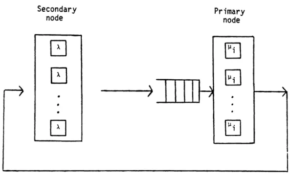
As mentioned in the introduction, the model under investigation is a two node closed cyclic queueing system. The primary node consists of M identical servers fed by a single queue. The secondary node, which provides a mechanism to model the arrival process is modelled as an infinite server queue.

Schemat-ically, this may be represented as follows

Secondary

node Primary_node

~

~

0

@

r7

.

)

H

,

·

/

•

·

.

·

0

~

Figure 2.1. The queueing model under investigation.

Customers are chosen from the primary queue by means of the First-Come-First-)erved (FCFS) scheduling discipline. Each customer can request more than one server; in

fact, a customer may require any number of servers up to the maximum of M. The

customer at the head of the queue remains in the queue until the total number of

this number. Since all the servers are identical, the particular ones allocated

is irrelevent. Note that the FCFS discipline may force customers (other than the first) to wait even though there may be sufficient resource available (and hence

idle) to service their requests. The advantage of the FCFS algorithm is that it prevents the undesirable phenomenon of "indefinite postponementll

• Note also that FeFS may result in several customers being able to enter service simultaneously upon completion of a service. Each customer monopolizes all the servers that have been allocated to him for a period of time that is exponentially distributed. At the end of this period, the customer simultaneously releases all this resource .

•

For the purposes of the model, we shall assume that a customer belongs to one of R possible classes (R < M). A class r customer (1 ~ r

2

R) requires r servers

simultaneously. To further generalize the model, we shall also assume that the exponential service time distribution may be class dependent.

At the secondary node, there is no concept of class. ,Each customer receives service which is exponentially distributed with rate A. Naturally, because of

the ample server property, no queueing takes place. On exiting from the secon-dary server, a customer proceeds to the primary server, but does not specify his class until he reaches the head of the queue.

There are no known analytical methods available for solving such a queueing system. We shall use numerical techniques to obtain a solution since the only other alternative, simulation, would be much too expensiveo The numerical approach

involves choosing an appropriate state description vector for the system; deter-mining the corresponding transition rate matrix, lee. the matrix whose (i,j) com-ponent denotes the rate of transition from state i to state j, and finally cal-culating from this matrix the stationary probability vector of the system, i.eo

Then

throughput (i.e. the number of customers served per unit time), the queue-length distribution and the distribution of the number of busy (or idle) servers. We

shall now outline the numerical procedure in somewhat more detail.

It is often possible to represent the behavior of a queueing system by des-cribing all the different states which it may occupy and by indicating how it

moves from one state to another in time. If the time spent in any state ;s exponentially distributed, or, in other words, if the probabilities of transi-tion depend only on the state currently occupied by the system and not on any previously occupied state, then the system may be represented by a Markov chain. Even when the system does not possess this exponential property explicitly, it is usually possible to construct a corresponding implicit Markov representation.

Consider a system which is modelled by a continuous time Markov chain. Let ~i(t) be the probability that the system is in statp. i at time t.

n n

c·

(t +dt) = E;.(t) (1- La ..dt ) + { L Qk· f;k ( t) )dt + 0(dt ) ,

, 1 j#i lJ k#i'

where a .. is the rate of transition from state i to state j, and n is the total lJ

number of states.

Define a. ••

11

n

= - La •.

j#i 1J

Then

n

;,.(t+dt) = E;,.(t) + ( E ak.~k(t)}dt + o(dt) k=l 1

and

i .e.

Lim [~.(t+dt)-~i(t)]/dt dt+O 1

n

~,.(t}

=

L ak·~k{t)

k=l 1

n

= Lim ( E aki~k(t)+o(dt)/dt),

dt+O k=l

where x(t) is a vector of length n whose ith component is (i(t) and A is a

matrix of order n whose (i,j) element is t_{i j ·}

At steady state, the rate of change of x(t) is zero, and therefore

T

A x = 0 ( 1)

The vector x ;s the required stationary probability vector (~i is the probabil-ity of being in state i at statistical equilibrium), and may be obtained by . applying equation solving techniques to the homogenous system of equations (1).

Note that ATx

=

0 => AT6t x + x

=

x

· e _'pTx

'l , •

~ T T

=

x, where P

=

A 6t+I

If 6t ;s chosen such that 6t _-< (maxln··I), then the matrix P is a stochastic

,

_{. 11} matrix. It may be regarded as the transition probability matrix for a discrete time Markov system in which transitions take place at intervals of 6t, 6t being sufficiently smal; to ensure that the possibility of two changes of state within

this interval is negligible.

We note that the matrix Qdefined as Q= _AT is a singular irreducible M-matrix with zero column sums. Such a matrix is sometimes called a "Q-matrix". The matrix A is called the infinitesimal generator or the transition rate

matrix. The system of equations, (1). is sometimes referred to as the station-ary form of the Chapmann-Kolmogorov equations, but more often simply as the global balance equations. Note that since this system of equations is homo-geneous, a zero pivot will occur during the last decomposition stage of

Gaussian elimination, (See Stewart [12]). However, we have not used the fact that the sum of the probabilities must equal one, (i.e. our normalizing equa-tion). Eliminating one of the equations from ATx =

a

and replacing it with

the normalizing equation yields a non-homogeneous system which indeed may be solved without pivoting, (See Stewart [12]). Alternatively, ATx

=

a

can be

Problems arise from the computational point of view because of the extremely large number of states which many systems may occupy. As will be

shown below, it is not uncommon for hundreds of thousands of states to be generated, even for simple applications. Since the matrices involved are

large and extremely sparse, numerical iterative methods such as Gauss-Seidel (either point or block) are usually recommended (unless, as sometimes happens, the non-zero structure of the matrix is highly regular in which case it may be

3. Generation of the Transition Rate Matrix

If we assume that there are R distinct customer classes, then we may

des-cribe the state of our system by the vector

(n, c1, c2, 0 • •' cr , .. 0cR )

of length R+l. Here n denotes the number of customers waiting in the secondary node, and cr denotes the number of customers of class r in service in the

pri-mary node.

Computer generation of the transition rate matrix requires the solution of three basic problems~ The first, is simply to enumerate all of the states of the system. The second, is to associate the proper enumeration integer with the vector description of any arbitrary state. The third, ;s to find all of the states which are accessible from an arbitrary given state (as well as the rate associated with each transition). These we have termed the "enumeration" problem, the "translation" problem, and the "transitionll

problem respectively. An enumeration is simply a listing of all possible vector state descrip-tions. The ordinal position of each state vector in an enumeration is called its state number. Now, all states with identical n parameter, i.e. all states with the same number of customers in the secondary node, are regarded as

form-ing a block. States within a given block are enumerated using the algorithm first reported in an earlier paper (see Fletcher, Perras, and Stewart [5]), where we studied a single node version of the queueing system considered here.

In

particular, states within a block are enumerated in a somewhat natural

The translation algorithm produces the correct state number for a given state vector. Due to the frequency with which it is called, it is perhaps the most time critical routine in the matrix generation procedure. The translation algorithm is implemented via a binary "dictionary" tree. The components of the state vector provide keys describing a path to the leaf which contains the associated state number. This algorithm was first reported in [5]. Each block of states is maintained in a separate tree~ Thus, there are as many trees as. blocks of states. For each state vector, parameter n furnishes a key

describ-ing which tree contains the state number.

The transition algorithm finds all the states which are accessible from an arbitrary given state as well as their corresponding transition probabilities. A state transition may be initiated by a departure from the primary or secon-dary node. Transitions due to a departure from the primary node are the most difficult to handle. This is because a departing customer may free up several servers, thus giving rise to different feasible combinations of customers that may enter service. Each of these combination of customers may correspond to a different state. The transition algorithm is primarily concerned with finding all these states. The key idea in this algorithm is the use of the displacement table. We digress for a moment to explain this idea.

We recall that a customer in the primary node does not specify its class until it reaches the head of the queue. Furthermore, the customer at the head of the queue (hereafter referred to as HOQ) has a class with a service require-ment exceeding the current number of idle servers. The remaining customers in the queue may be of any class. Now, upon departure of a customer from the pri-mary node, the total number of idle servers is increased. The new idle resource may exceed the HOQ requirement, in which case the HOQ will enter service. Now, the new HOQ may be of any class. We call the system configuration at this point

end

primary node, can be easily determined using this base state. In particular, they can be determined by examining the various combinations of customers (waiting in the queue) that can enter service. The vector description of each of the resulting states may be regarded as a displacement of the base state vector.

In

fact, the set of possibilities for how many of each customer class may enter service can be described numerically by a set of vector displace-ments. The crucial observation here is that this set of displacements depend' only on the excess service resource available and the length of the queue. It does not depend on the base state~ Our algorithm capitalizes on this fact by maintaining a displacem~nt table in memory which it consults to facilitate the generation of state transitions. Each transition represented in the displace-ment table has an associated rate which is also stored in the table.

The operation of the transition algorithm may be summarized as follows.

if (secondary node is nonempty) then assume departure from secondary node if (queue is nonempty) then

customer enters queue

** '

else

for (each customer class) do

if (service requirement exceeds available resource) then customer waits in queue

**

else

customer enters service

**

if (primary node is nonempty) then

for (each customer class in service) do

customer departs service enters secondary node

if (HOQ requirement exceeds current available resource) then queue is unchanged

**

else

HOQ will enter service

for (each entry in the displacement table consistent with available resource and queue length) do

HOQ and (perhaps) other customers enter from queue

**

**

indicates that

- A new accessible state has been reached.

The actual implementation of the algorithms requires the use of many con-trol variables to keep all of the necessary information current as well as the data structures required for the dictionary trees and the displacement table. We sketch the procedure for generating the matrix in terms of the algorithms which we have discussed.

For a given set of system parameters (# customers. # servers, # classes, etc.) the enumeration algorithm generates the vector description of each state (matrix row) which is possible.

For each of these possible states the transition algorithm generates the vector description of every accessible state together with the associated transition rate.

The state number (matrix column) for each accessible state ;s provided by the translation algorithm allowing the transition rate to be placed in the correct matrix entry.

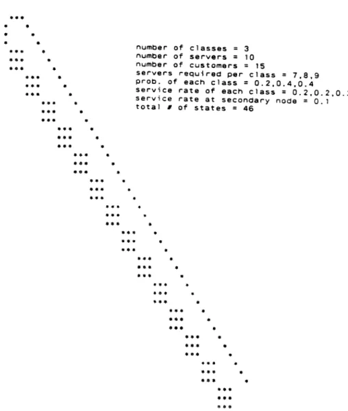
An examination of the transition process will reveal that all of the states accessible from a given state will either be in the preceding block (in the case of a departure from the primary node) or in the succeding block (in the case of a departure from the secondary node). Thus the rate transition matrices which we generate will all have a block tridiagonal structure. Our solution technique

4. The Numerical Approach

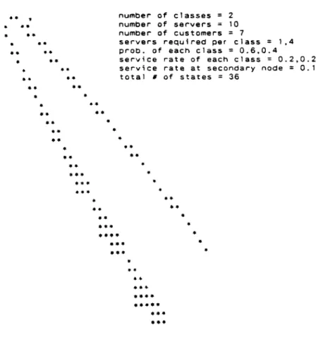
When the states of the system are arranged according to the order prescribed in the previous section, the transition rate matrix will possess a block tridiag-onal form. Some examples obtained from a number of different cases are presented

in figures 401 through 4.4 below.

••• • • • • •

.*.

•

.*.

• *0* _• ••• ••• ••• • • •

...

• ••• • ••• • ••• • •••

..

••• • ••• ••• ••• ••• * •• •••

number of classes =3

number of servers

=

10

number of customers = 15

servers required per class = 7,8,9

probe of each class = 0.2,0.4,0.4

serv~ce rate of each class =0.2,0.2,0.2 serV1ce rate at secondary node =0.1

total # of states = 46

*** •••

*.. ..

....

••• •••

....

.

••• ••• ••• • * •

...

• ••• •

....

..

••• • ••• • •••

..

••• • ••• ••• •••

..

••• * •• $*.

•• •••

....

....

•• ••

..

••• ••• •

..

• •••

.

..

• •

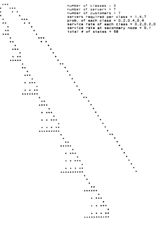
number of classes - 3

number of server~ = 7

number of customers 7

servers required per class 1,4,7

probe of each class = 0.2,0.4,0.4

service rate of each class = 0.2,0.2,0.2 service rate at secondary node = 0.1

total # of states =58

• • • •• ••••• •• •

..

..

..

...

•

...

..

...

• • •

..

• •

..

• •

-..

•

..

••

..

..

•

-.

...

~.*

...

•

...

••

•••• • ••• •

..

.. .. * ••

.

..

..

•• •••••• •

....

•

..

...

•

..

.

..

...

.e.

• • ••• • ••• •• • • ••• •• • • • •• • ••• • •

....

• •••

..

. . . $ * •••• ••

..

••• • • • ••

...

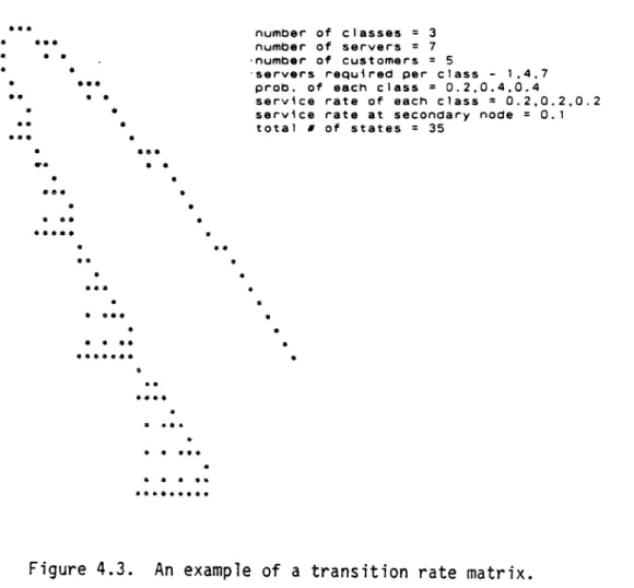
number of classes =3

number of servers =7

'number of customers 5

'servers required per class - 1,4,7

probe of each class =0.2,0.4,0.4

service rate of each class =0.2,0.2,0.2

service rate at secondary node = 0.1

total # of states =35

..

• •

..

•• • •

..

• •

..

...

..

...

• • •••

..

..

..

.

..

•••••••••

number of classes = 2 number of servers; 10 number of customers = 7

servers required per class

=

1,4

probe of each class =0.6,0.4

service rate of each class =0.2,0.2 service rate at secondary node = 0.1 total # of states =36

..

.

•• • •• •• *• •• • •

..

•

..

..

..

•• *• • •• ••

....

•• * • •••••

....

••• ••

•

•

..

•• •• * •• •••• * •• *•• •

...

...

**. *•• •• * •• y ••

..

•• •• •• •• • •• ... _••

...

•• •• ..

.

•

We shall use the following block notation to represent these matrices.

AOO AOl

A

10 A11 A12 (Zero)

A

A

2 l A22 A23 .•••

=

(Zero) A " · A · · · · A_{N-l,N-2 N-l,N-l N-l,N}

AN,N-l ANN

The number of blocks, N+l, is obviously related to the number of customers N t~at circulate in the network; block j is associated with states in which j CJstomers are at the primary node. If n· is the number of such states, then

J N

the order of the transition rate matrix A is given by n= t n

Jo • Notice that the j=O

diagonal blocks are themselves diagonal submatrices. As we shall see below,

t~is, together with the fact that the diagonal element in each row is equal to

the negated sum of the off diagonal elements in that row, makes the block Gauss-Seidel method extremely attractive as a means of solution.

We shall assume that the stationary probability vector x and successive iterates x(s) to the solution vector are partitioned conformally with A:

i .e. and

T (T T T) e- IRn

x

=

_{xO,x" ... ,xN} ~

n. N

x. e: IR J with 1: n. = n 0

J j=O J

For s

=

0, 1,2 , . .. (untt1 convergence) For j =0,l,2, ...,N

S 1o ve A ..x .(5+1) -- -A.. 1x .(s+l)1 - A.. 1x •(s)1

JJ J JJ- J- JJ+ J+ (4.1)

where it is implicitly assumed that the matrices A_{j j_}

1 and Aj j+l are identi-cally zero when j=O and j=N respectively.

Since the diagonal blocks of A are known to be nonsingu1ar and are diag-onal, their inverses, Aj} j=O,l ••• N, may be trivially computed and hence equation (4.1) may be written as

x(. s+1) -1 (5+1) -1 (s)

=

-A · .A .. lX' 1 _{- Ajljj+1Xj+l}

J JJ JJ-

J-i . e. _x.(x+l)

=

V.x~s+l) + W.x~s)

J J J-l J J+l

Note also that Vj and Wj may be computed before the iteration procedure

is initiated, so that it is not necessary to store the diagonal elements

explicitly during the actual computation of the stationary probability vector. Schematically, the matrix is then as follows

W₂ 0

.

.

_V2•

.

.

.

.

.

.

.

.

.

.

.

.

.

.

.

..

.

.

.

.

.

W 0

V

_N-

1

n

0 WT₁

V₀T 0 WT₂

VT₁ 0 WT

0

.

3.

..

.

•

.

Cl

.

0

V~_2

a

w~

T

V

_N-

l

a

Since the iteration vector x{s) ;s similarly partitioned, the effect of perform-ing an iteration may be viewed as the product of

0 WT₁ X

o

(

.

)

VT 0 WT

o .

₂ xl(

.

)

.

Cl

WT

0 0

0 • N

T · (

.

)

VN- 1 0 xN

with the only difference being that as portions of the new iterate are formed they are used in all succeeding computations rather than the values of the pre-vious iterate.

In the absence of any better information, it is suggested that the initial approximation be taken as

(l

1

5. A Sparse Storage Scheme and Other Implementation Consideratio~s

We now turn to a discussion of the sparse storage scheme which ;s used to store the non-zero elements of the transition rate matrix. Given the size of the matrices involved, such schemes not only make sense from a spdce saving point of view, but are often prerequisite if a solution at all is to be obtained.

Given the form of the matrix equations presented in the previous section, it should be noted that the only operations required of the elements is multipli-cation with a vector. Consequently, the storage scheme used should make such a product convenient. However, other considerations must also be a~commodated; in particular, the manner in which the non-zero element themselves are generated. Recall that the element Q

i j of the transition rate matrix denotes the rate of transition from state i to state j and that the matrix generation procedure obtains all possible transitions from a given state before proceeding to deter-mine transitions from the next state. As a result, the matrix A is generated by rows. However, the stationary probability vector x which we are seeking is the solution to ATx=O, which involves the transpose of the transition rate

matrix.

We shall therefore store the non-zero elements by rows as they occur but when performing the multiplications during the iteration phase, we shall need

to remember that it is the transpose that ;s used.

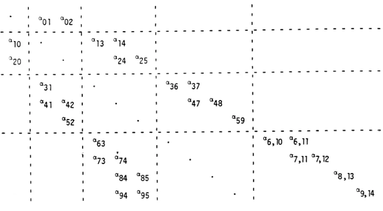
We shall describe the sparse storage scheme which we recommend by means of the following example, which has the structure of the upper left hand portion of a typical transition rate matrix for this application. The diagonal elements

-

.-I

-.-

-

- - -

- -

-

-

~

-

- -

-

-, I

~

-

-

-

-

_I

-I

"s,

10 Q6, 11

Q7,11 Q7,12

,

Q

73 a74

QS4 aSS

Q

94 Q95

__I ..

-

-

-

--

_I

Q

31

a

41 a42 I a_SZ I

..! - - -

-':l20 I

Figure 5.1. Upper left-hand portion of transition rate matrix for

We shall use a real, one dimensional array V to store the non-zero elements of

the upper triangular portion and an integer array IV to indicate the row/column

position in the matrix of these elements. Areal array Wand corresponding

integer array IW will have similar functions for the lower triangular portion.

The negated recriprical of the diagonal elements will be stored in a real array

0; obviously no integer array is required. Also, once the products

-A~~A

.. 1

JJ

JJ--1

and -AjjAjj+l have been computed, the diagonal elements are no longer needed

and the array 0 should be used to hold the iteration vector.

of row k-1 (viz. a

k- 1, j ) . The order of e1emer.ts within each row is immaterial. The integer array IV will denote first the number of non-zero elements in a given row and then the column position of each of these elements. Obviously this latter must correspond to the ordering in V. Thus, for example, one possible ordering is

I I

°13°14 °24°25 °36037

:a14,8a14,7~ Q59

..

..

]

IV [2 2 1

!

2 3 4

t

2 4 5

~

2 6 7

!

2 8 7 : 1 9

! .... ]

I I I I I 1

Asimilar arrangement holds for the non-zero elements in sub diagonal blocks. As the non-zero elements are being generated and inserted into the arrays

-1

Vand W, it is possible to incorporate the effect of the multiplication by -A ..

JJ

simultaneously. The effect of the multipliCation ;s to multiply all of the

ele-, n

ments in a given column, column k say, by ---- where 0kk

= -

E o-k. (Note

C).k i=l 1

column i, not row i, since we require the transpose of the matrix). For the elements in subdiagonal blocks, this multiplication may be performed as soon as the elements themselves are determined and tre product may be stored directly into W. This is because the required diagoncl element will always have been previously generated. This is not true for non-zero elements in the super dia-gonal blocks so that it will always be neces~ary to backtrack a little. For example a

12 and a13 must be multiplied by a22 and a33 respectively, but neither

a

22 nor a33 will be available until the second block has been completed .• It now only remains to show how the product W_j+_1xj+_{1 (or Vj _1}X_{j_1)} is to

be carried out given that W_j+

w

31 Va _{[val v02]; W2} = w w

41 42

w

52

xO

~~

C3

(E;O] ; _Xl = x - t 4

2

-C

s

V

o

is stored as

V: [val' \1₀₂

.

.

.

..

]

IV: [ 1, 1, 1, 1 ]

while W2 is stored as

W: [

....

w

31 w41 w42 wS2 ]

I

]

IW: [

....

1 2 1_{I 2} 2 _I

....

I

It may easily be verified that the required result is given by

f;(s+l) ₌ w f;(s) + w f;(s} +" c(s+l)

1 31 3 41 4 01 0

r; (S+1)

= w E;(s) + (.)

c(

S ) + v f::(s+l)

2 41 4 52 5 02 0

One possible procedure is to first zero out the components of

x~S+l);

i.e.

~~S+l)

=

~~S+l)

=

0, and to add parts of the result into the appropriate position as and when they are obtained. Consider, for example, how

w~x~s)

is formed and added into

x~S+l).

The plements in the array Ware processed one at a time. For

each element in this array we must determine the appropriate element in

x~s)

with

row ~rocessed. Thus w

3l ;s multiplied by ~3' the next two elements w41 and w42 are Joth multiplied by 44 and finally w

S2 is multi~lied by 4S. Thus we see that both the arrays Wand x are processed linearly. Once each of these

multiplica-t;o~s have been performed, the result must be added into the appropriate position

of xl(s+1) · Again the determination of the correct position is easi1y 0btalne. d

by progressing linearly through the array IW (remembering that the actual position indicators are preceded by the number of elements. Thus

W31~3 is added into position w41~4 is added into position w42~4 is added into position 2 w52~4 is added into position 2

(5+1) · (s+l)

The product Voxo may be computed and added lnto xl in a similar fashion.

Thus we see that although the matrix is not stored in the most obvious fashion for multiplication with a vector, such computations may still be

6. Numerical Results

The numerical procedure outlined in the previous sections was implemented on a VAX 11/780. Numerical experience with this procedure showed that most of the processing time was devoted to the matrix generation procedure. The

calcu-lation of the stationary probability vector required only a small fraction of the total processing time. Complicated configurations requiring more than two classes of customers and a large number of servers were easily analyzed. Time complexity limitations became apparent only when there were R classes present, where R is greater than 10. In such a case, one can still use the algorithm effectively by reducing the number of classes to a more manageable level. Such a reduction can be achieved by appropriately lumping classes of little opera-tional interest into a single class.

It has been observed empirically that the blocks on the lower diagonal in the transition rate matrix are all identical after a certain block. In parti-cular, they are all identical after the block number lM/rOJ+l, where Mis the number of servers in the primary node, and r O is the smallest permissible class (ro:l). In view of this, one may not need to generate all the lower diagonal blocks. For example, in figure 4.1 it suffices to generate the first two lower diagonal blocks, seeing that all the remaining blocks are mere repetitions of the second block. This particular behaviour can lead to substantial savings in processing time when generating the rate matr;xe Obviously, in order to avail of this saving the number of the lower diagonal blocks that have to be gener-ated should be greater than LM/rOJ+l.

The numerical procedure was employed to obtain various measures of perfor-mance as shown in figures 6. 1 to 6.6. The number of servers in the primary node was fixed to 15. A customer in the primary node may require 1, 4, or 7

under study were varied in order to obtain the results shown in the figures below. These parameters are: a) number of customers in the system; b) the

vector (~1'~4'~7) of service rates of customers class 1, 4, and 7 respectively; and c) the mean service time at the secondary node 1/~. The performance mea-sures obtained are related to the primary node. These are the throughput, the mean queueing time and the mean number of busy servers. The throughput is defined as the average number of service completions per unit time.

Figure 6. 1 gives the throughput of the primary node as a function of the number of customers in the system plotted for various values of (~1'~4'~7).

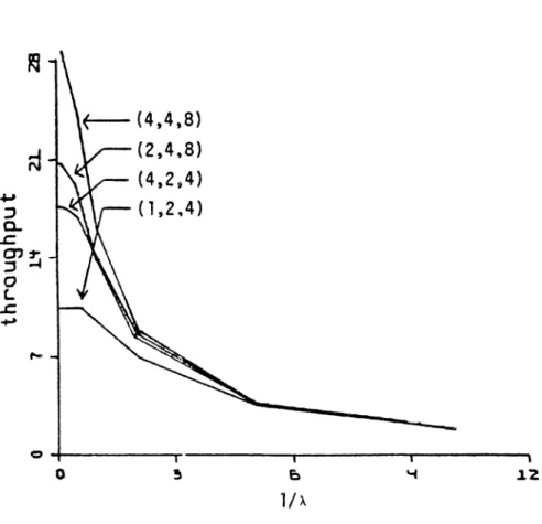
Figure 6.2 gives similar information for the throughput, but as a function of

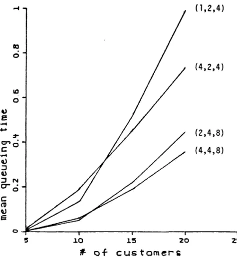
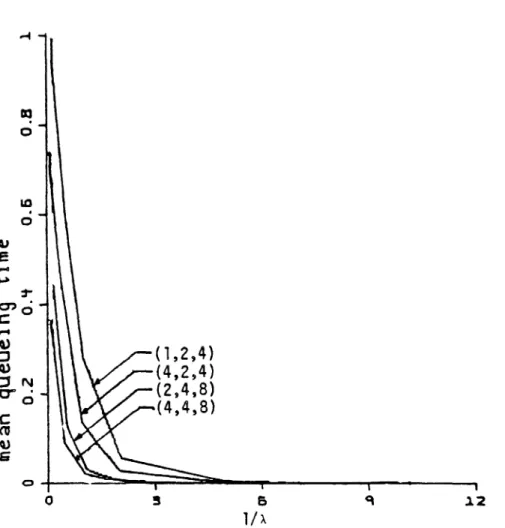
l/A. The mean queueing time in the primary node ;s given in Figure 6.3, as a function of the number of customers in the system plotted for various values of (~1'~4'~7). Figure 6.4 gives similar information for the mean queueing time, but as a function of l/A. Figure 6.5 gives the mean number of busy servers at the primary node as a function of the number of customers, plotted for various values of l/A. The same information, but slightly rearranged, is given in

Acknowledgement

(4,4,8)

(2,4,8)

~~

_Q..

..&:.

en

::J

0

r,

In (2,2,4)

.s: _~ ~

(1,2,4)

II"-t---...,...---...---o 5 1.0 1.5

,. of cu~tomers

20

( - - (4,4,8)

(2,4,8) (4,29 4 )

....,

~ (1,2.4)

a.

s:

g'~

o

t.

s:

~

e -t---~---y---w---~

o D

1/A

Figure 6.2: Throughput of the primary node vs. mean service time at the secondary node, plotted for various values of (~1'~4'~7); the number of customers

I:J

o

10

0

~

e

...

....

7

c:::r" •

C 0

....

to)

:J

t)

:1 N

cr- •₀

C

CV

\J

S

0

5 ~o 15 20

,. of customer;

(1,2,4)

(4,2,4)

(2,4,8) (4,4,8)

25

111 o

LO_,

o

~

0 ' ) •

c: 0

.f1""4

t)

:J

Q)

:7 N

tT _o·

C

CU

"

Ei

6

1/A

q _.12

10

....

In

'-_.u

~ _N

1- ~

QJ

(J)

~

(J

='

ttl

.D

'+

0 ~

C

:I-eu

QJ

1:

0

0 5 ~o ~!5 20

f

of

cUSDtomer~

Figure 6.5: Mean number of busy servers at the primary

node vs. the number of customers in the system, plotted for various values of l/x;

en

C-Q.l N

> ...

t...

Q)

<It

c-+---.---...---.

o

l/A

9 J.Z

Figure 6.6: Mean number of busy servers at the primary node vs. mean service time at the secondary nodet

References

1. Arthurs, E. t and Kaufman, J. S.t IISizing a message store subject to blocking criteria", in Performance of Computer Systems. M. Arata, A. Butr;menko, and

E. Gelenbe, (Eds.), Amsterdam, The Netherlands, North Holland, (1979) 547-564. 2. Brill, P. H., and Green, L., tlQueue in which customers receive simultaneous

service from a random number of servers - a system point approach", Mgmt. Sci., 30 (1984) 51-68.

3. Brill, P. H., ItAn embedded level crossing technique for dams and queues", J.

of App1. Prob., 16 (1979) 174-186.

4. Federgruen, A., and Green, L., "An M/G/c Queue in which the number of servers required is random", Columbia Business School Research paper 504A, Columbia University, (1983).

5. Fletcher, G. Y., Perros, H. G., and Stewart,

w.

J., itA queueing system where customers require a random number of servers simultaneously", CCSP-84l2, Computer Science Dept., N. C. State Univ., (1984).

6. Gopal,

I.

S"I and Stern, T.

E.,

"Optimal call i'locking policies in an inte-grated services environment",

IBM

Research Report RC 9825.

7. Green, L., IIA queueing system in which customfrs require a random number of servers", Opere Res., 28 (1980) 1335-1346.

8. Green, L., "Comparing operating characteristics of queues in which customers require a random number of serversll

, Mgmt. Sc~., 27 (1981) 65-74.

9. Kaufman, J., IIBlocking in a shared resource environment", IEEE Trans. COrml., Com-29 (1981) 1474-1481.

10. Kim, S., "M/M/s queueing system where customers demand multiple server use",

Ph.D. dissertation, Southern Methodist Univ., (1979).

11. Schwartz, M., and Kraimeche, B., ItAn analytic control model for an integrated node", Inforcom 183 San Diego, (1983).