A procedure for the computation of seismic fragility of equipment components in NPPs

20th International Conference on Structural Mechanics in Reactor Technology (SMiRT 20) Espoo, Finland, August 9-14, 2009 SMiRT 20-Division 7, Paper 1904 A Procedure for the Computation of Seismic Fragility of Equipment Components in NPPs

Federico Perottia, Marco Domaneschia and Silvia De Grandisb

a

Department of Structural Engineering, Politecnico di Milano,Italy, e-mail: [email protected]

b

SINTEC srl, Bologna, Italy

Keywords: Seismic fragility, Isolation techniques, Dynamic analysis.

1 ABSTRACT

The research work here described is devoted to the development and testing of a numerical procedure for the computation of seismic fragilities for equipment and structural components in Nuclear Power Plants (NPP). Given the very low damage probabilities which are required in modern nuclear industry, attention is focused on the comparison between the performance of traditional and seismically isolated buildings. The procedure is based on the hypothesis, typical of nuclear structures, of linear behaviour of the building in the traditional case; the behaviour of isolation devices, on the other hand, is modelled taking mechanical non-linearities into account.

The proposed procedure for fragility computation makes use of the Response Surface (RS) Methodology to model the influence of the random variables on the dynamic response. To account for stochastic loading the latter is computed by means of a simulation procedure. Given the RS, the Monte Carlo method is used to compute the failure probability; a risk-based procedure for refining the RS is also proposed and tested in an illustrative example. For the isolated case, an overall experimental/numerical methodology for fragility assessment is finally sketched.

2 INTRODUCTION

Accident scenarios initiated by external events are becoming the leading contributors to the overall estimated Core Damage Frequency (CDF) for modern Nuclear Power Plants, given the very low CDF associated to internal events (Maioli et al, 2005). Among external events, as demonstrated by a large number of Probabilistic Risk Assessment (PRA) studies, earthquakes play a very important role. In such situation a high level of attention on issues related to seismic behaviour is required at all design stages; on the other hand, unnecessary conservatism must be removed, as much as possible, from seismic risk analysis.

Within the context of conceptual seismic design, the adoption of isolation systems seems to be almost mandatory if the earthquake-induced CDF must drop to values of the order of E-08/ry. In this respect, isolation systems based on High Damping Rubber Bearings (HDRB) represent a highly reliable design solution, given their diffusion and proven reliability; in a parallel paper (Perotti et al, 2009) the application of this solution to the Nuclear Steam Supply System (NSSS) building designed within the IRIS international project (Carelli et al, 2004) is described and some preliminary results are given. These results shown how the isolation system is extremely effective in reducing the seismic acceleration transmitted to all structural and equipment components inside the building; in such conditions the isolation devices themselves are prone to become the critical components in terms of seismic fragility, since the response attenuation is obtained as the result of large relative displacements between the building and the foundation.

When the problem of risk evaluation is addressed, the fundamental role played by the hazard definition in the estimation of the seismic-induced CDF is immediately evident; both randomness and uncertainty, however, significantly affect also the evaluation of structural behaviour under extreme loads and thus of seismic reliability. Though randomness cannot be avoided, since is inherent to most of the input data of the analysis, uncertainties, being related to the lack of complete and accurate knowledge about models and methods, must be reduced as much as possible by refining analysis procedures.

traditional design approach and in the case of an isolated building. An innovative procedure for fragility estimation (De Grandis et al, 2008) will be summarized in the next section and further developed focusing on the isolated case; an example of application will be shown with reference to a traditional design. Criteria for the probabilistic evaluation of isolated building will be finally discussed.

3 FRAGILITY ANALYSIS OF NPP BUILDING COMPONENTS

Following the PEER (Pacific Earthquake Engineering Research) approach (see Der Kiureghian, 2005 and references herein), the annual failure rate for a mechanical component under seismic loading can be obtained from the integral:

{

}

f f EDP IM

P =

!!

where DM is a Damage Measure, associated to the assumed limit state (dmf denotes the damage level at

failure), EDP is an Engineering Demand Parameter (support acceleration, relative displacement,…) expressing the level of the dynamic excitation imposed to the component due to the global seismic response of the structure (reactor building) and IM is an Intensity Measure (peak ground acceleration, spectral acceleration,…) characterizing the severity of the earthquake motion at the reactor site. As pointed out by Der Kiureghian (2005) all statistics in (1) must be intended in term of annual extreme values, so that the equation delivers a risk estimate in terms of annual probability of failure of the component. For a “simple” equipment component, or for a preliminary evaluation, the limit state can be directly defined in terms of the EDP value at failure edpf, thus avoiding the damage analysis step, i.e:

{

}

f f IM

P =

!

We shall denote in the following the fragility function F(edp,im) as:

{

}

( , ) 1 _EDP( / )

F edp im =P EDP>edp IM =im = !P edp IM =im (3)

where P_EDP(edp IM/ =im) is the conditional CDF of the edp random variable.

3.1 Linear case: traditional building

For equipment components located inside a non isolated reactor building of a NPP, we shall consider as EDP the extreme value A, of the absolute acceleration at the component supports; the peak acceleration Ag of the

most severe component of horizontal ground motion (PGA) will be taken as IM. We shall assume that the damage analysis can be performed by studying the equipment component under the dynamic excitation defined by the time-histories of support accelerations, having a peak value equal to A. The support motion can be in turn computed by studying the building response via a structural model in which the component is represented in a simple way (rigid mass or simplified model). This implies that no significant structure-equipment dynamic interaction occurs. This is particularly attractive when, as it usually the case, elastic behaviour can be assumed for the reactor building, so that non-linearity can be confined within the component damage analysis.

The fragility function can therefore be interpreted, in the linear case, as the probability of exceeding a given structural dynamic amplification, that is:

{

}

( , ) _{g g exc}( , _g) _exc( / _g)

F edp im =P A>a A =a =P a a =P a a (4)

For stochastic seismic input, the exceedance probability (4) is associated to a limit state function which can be written in the following “safety margin” format:

( , , g) ( , g) ( ) g 0

g X a a =C!D X a =a!R X a = (5)

where g( , ,X a a_g) is the performance function, X is the vector listing the random variables (RV) and R(X)

parameters and the structural properties, the probabilistic description of R is the result of a random vibration analysis. Expression (5) can be rewritten as:

( , / _g) / _g ( ) 0

g% X a a =a a !R X = (6)

in which the peak amplification factor a/ag is explicitly stated as EDP. Once selected the probability

distributions of X and R the probability of exceeding the limit state (6), i.e. the integral

0

( /

)

( , )

exc g R

g

P

a a

p r

dr d

<

=

!!!

x

x

%

(7)

could be computed, in principle, by direct application of the Monte Carlo Simulation (MCS) method; in fact the statistics of response R(X) is algorithmically known, i.e. can be deterministically computed by structural dynamic analysis for every realization of the random variables X. It must be considered, however, that a huge computing time and cost would be required for running a complex finite element model, as it is the case for a NPP reactor building, for the number of evaluations which are necessary for MCS, especially for the estimation of small probabilities.

For the above consideration, according to the well-established Response Surface Methodology (RSM - Faravelli, 1989, Casciati, 1991), the “true” response function is replaced by a simple analytical representation. Here, assuming that the distribution of R can be described by its mean value µR and its

standard deviation σR, the so called “dual response surface” approach (Towashiraporn, 2004) has been

adopted for modelling their dependency on X. Assuming that the same model can be used for the mean and the standard deviation the following response functions have been introduced:

1

( ) ( )

m

R i i

i

a z _µ

µ !

=

=

"

X X (8a)

1

( ) ( )

m

R i i

i

b z _!

! "

=

=

#

X X (8b)

where the ai’s and bi’s are coefficients to be estimated, the zi’s are usually polynomial functions and two

“error” terms (εµ , εσ) are introduced as a zero mean random deviations. The latter account for the variability of estimated quantities and for the lack of fit of the adopted model, i.e. for the inadequate analytical form of the RS’s and for missing variables (i.e. not comprised in (8a,b) though influencing the response). To compute the coefficients in (8a,b) a number of experiments must be run according to the chosen experimental design; at each of them the random vibration problem can be addressed via either an analytical or a simulation approach. In the second solution, here adopted, a sample of ground motion realizations must be generated, according to the spectral parameters appearing in X. For each realization, the extreme value of R is computed (e.g. via FE modelling and step-by-step analysis); the mean and variance of R are then estimated. The procedure is repeated for all experimental points, leading to n observed values for the statistical parameters of R(X).

We shall assume in the following that the experiments are performed in homogeneous conditions (i.e. differing for the xi values only), that their results are independent and that the error terms are normal with

constant variance; under these hypotheses an unbiased estimate of the coefficients ai,bican be obtained by

the Least Square (OLS) method, independently of the variance of the !’s. An unbiased estimate of the latter terms can be subsequently obtained is defined, in terms of the residual values. Once models (8a,b) are established, MCS can be carried on. Note that to compute the fragility curve (4) the integral (7) must be evaluated for a number of amplification values a/ag, even though the Response Surface estimates (8) remain

the same.

3.2 Non-linear case: isolated building

therefore the extreme value u of the relative displacement across the most strained isolator will be initially taken as edp. The fragility function is therefore expressed as:

{

}

(

,

)

( ,

)

F edp im

=

P U

>

u A

=

a

=

P

u a

The associated limit state function can be expressed in the following “capacity minus demand” format:

( , , g) ( , g) ( , g) 0

g X u a =C!D X a =u U! X a = (10)

where U is the random variable whose distribution delivers, for fixed X, the result of the random vibration analysis. Note that no linearization is here exploited, since the behavior of HDRB is markedly non-linear, especially at the high level of deformations here anticipated. For a fixed value of ag, however, the same

criteria as applied, in the previous section, to the random amplification R can be here used for the random response U, whose properties can be modeled, through appropriate Response Surfaces, as functions of the basic random variables X. Once expressions of the type of (8a,b) are established and given the properties of the basic random variable, MCS can be applied to the evaluation of the integral delivering the exceedance probability as

0

( , ) ( , )

exc g U

g

P u a p u du d

<

=

!!!

Differently from the linear case, however, the Response Spectra evaluation must be repeated for every value of peak ground acceleration, this representing, potentially, a huge computational task. It can be considered, however, that in the isolated case the seismic behavior of the building can be captured, to the aim of evaluating the isolators’ behavior, by means of very simple mechanical models; the latter, in fact, can be based on the hypothesis of rigid-body motion of the building above the isolators.

Note that, at a second stage of the research program, a more refined approach will followed, based on the definition of a failure domain for the isolator, expressing the interaction between vertical and horizontal force; this will allow for assuming an improved formulation of the limit state function (10).

3.3 Experimental design

If second-order models full models are used for the Response Surfaces, the estimation of

(

)

1 1 / 2

p= + +m m m+ coefficients is required for m random variables. The adopted experimental strategy is

here the “Central Composite Design” (CCD); once fixed a “center point”, CCD is the combination of a classical “two-level factorial design”, in which all the combinations of two levels (high/low) of the rv’s are considered, with a “star design”. In the latter 2m points are considered in which one variable takes an intermediate value and the others are at the central value. Including the central point, a total number of experiments equal ton=2m+2m+1 is reached; if m=3, for example, we have p=10 and n=15.

In terms of non-dimensional zero-mean random variables

(

)

i i

i xi x x

! = #µ " , high and low levels are usually fixed in the range !_i = ± ÷(1 3), while for preserving the “rotatability” of the design the star points

must be placed at 4

2k

! = ±

3.4 Risk-based refinement of the fragility computation

In reliability problems the refinement of the Response Surface aims to an improved fitting in the region of the failure domain where f (X) gives the largest contribution to the failure probability. An obvious choice, in this light, is to assume as design center the design or minimum norm point; this is defined by first transforming the RV’s into the space of standard normal variables Yi. Subsequently, the limit state function is

expressed in the same space and its point which is closest to the origin is found; this can be also interpreted as the “most likely failure point”. Obviously, the design point is not known when the analysis is started, so that an iterative refinement procedure is required in principle.

computation of the risk according to (2). If we consider the latter, along with expressions (3) and (4), we can write the probability of failure, for a given reference “capacity” edpf and for the site at study as:

( , ) ( ) (

)

g

f f A g g

P =

!

It can be noticed that, once edpf is fixed and a first evaluation of the fragility function is available, the

integrand function in (12) can be analyzed and the PGA range giving the maximum contribution to the total probability can be detected; for the general non-linear case (11) this directly states where the refinement the Response Surfaces must be pursued. In this sense the design point corresponding to the PGA leading to the maximum of the integrand function in (12) can be assumed as reference point.

For the linear case, given af the “dominant” PGA range delivers a range of amplification values, and

thus of design points on the different limit state surfaces, which can be considered for refinement.

For a practical implementation, the FORM technique, which has no significant cost once the design point is found, is an obvious choice for the evaluation of the fragility; the Rosenblatt Transformation has been here applied to deal with the correlation between the random response R and the other rv’s, while the error term has been disregarded during the refinement process. In addition, a type I extreme-value distribution has been assumed for the extreme value of random dynamic response (either R or U).

The procedure for fragility evaluation can be thus subdivided into the following steps.

1. Performance of a first set of experiments by centering the CCD at the average values of the rv’s and by assuming high/low levels at !_i = ±3.

2. Estimation of the coefficients of the RS’s expressing the mean and variance of R (or U).

3. Performance of FORM analysis for evaluating, for each amplification value in the range of interest, the design point position and estimating F(edp,ag).

4. Computation of the integrand function F(edp,ag)pA(ag) and selection of the PGA range in which

refinement must be pursued.

5. Performance of a new sets of experiments with high/low levels smaller than in step 1, covering the range of design points corresponding to the PGA range detected in step 4.

6. Back to point 2 for iterating the procedure.

7. Once the refinement procedure is ended the final value of the fragility F(edp,im) is computed via MCS; error terms are obviously included in the final version of the Response Surfaces (8).

4 TRADITIONAL BUILDING (LINEAR): EXAMPLE OF APPLICATION

The above described procedure has been applied to the analysis of a preliminary early design of the auxiliary building of IRIS (International Reactor Innovative and Secure). This is a medium power (∼335 MWe) pressurized light water reactor under development by an international consortium which includes more than 21 partners from 10 countries, led by Westinghouse Electric Company (see Carelli et al, 2004). Installation in a site characterized by a low-to-average seismicity level has been here assumed.

4.1 Structural and seismic input modelling

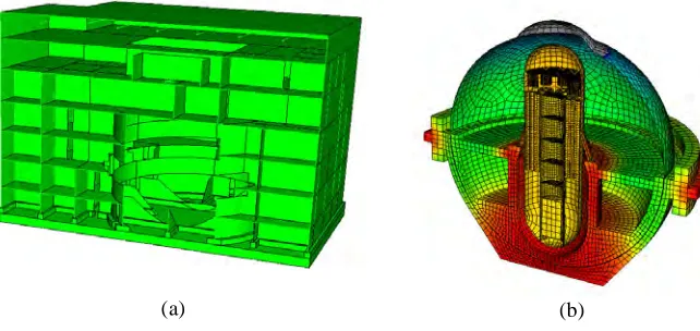
Details on the criteria adopted for setting dynamic models for the seismic analysis of the building can be found in (Bianchi et al, 2007); for performing repeated analysis, as here required, a “simplified” FE model has been set, encompassing about 5x105 degrees of freedom. The model is based on simplified approaches for representing soil-structure interaction effects and sloshing effect in RWST pools; shell finite element are introduced for modelling all walls and slabs, including the foundation mat (figure 1a). In addition, based on the results obtained by a more refined model (see figure 1b) the lowest part of the containment structure is considered as a rigid body, while the upper part (steel liner) is replaced by an equivalent two-degree-of-freedom system.

reference point for computing the extreme value of acceleration A, assumed as EDP. The natural frequencies of the first vibrations modes, encompassing significant soil deformation, range between 2 and 5.2 Hz. The vessel modes have frequencies in between 13 and 30 Hz.

The response spectrum prescribed by Eurocode 8 (CEN, 2005) for a type I earthquake and for local soil conditions type C was adopted as seismic input. The spectral parameters where treated as deterministic, so that a single set of ten input motions, each described by three components, has been generated and used at all experimental points. Generation was performed starting from real accelerograms and iteratively correcting their Fourier Amplitude Spectra in order to match the EC8 curve.

Figure 1. Reactor building (a), containment and vessel (b)

4.2 Random variables, RS model and experimental design

For a preliminary test of the procedure (see De Grandis et al, 2008) only three random variables have been here selected to represent the main sources of randomness for the computation of the response of an equipment located inside the vessel:

• a random variable (lognormal distribution) describing the soil shear modulus Gs, with mean value of 200

MPa and c.o.v equal to 0.2;

• a random variable (lognormal) for the vessel damping factor, νv; the mean value of νv has been chosen

equal to 0.03, and a coefficient of variation of 0.2 has been considered;

• a random variable (lognormal) to describe the viscous soil damping; more in detail, the ratio between the actual value and the nominal value of each damping factor associated to foundation modes is considered, named δ, with a mean value of 1 and a c.o.v. of 0.2.

It must be noted, with respect to the last two RVs, that damping has been here treated in a simplified way. This was due to the difficulty to deal with composite damping, by means of the software package at hand, within modal superposition analysis. In the case here shown, modal damping factor were directly stated and given in input by recognizing, with some engineering judgement, modes dominated by foundation or by vessel movements. As a result, nominal damping factors imposed to the foundation motion components were equal to 20, 7 and 10% for vertical, mixed translation-rotation and torsional modes respectively. Damping of other modes was fixed at 5%.

The model chosen for the mean and variance (8) of the dynamic response is a complete second order polynomial; a cubic mixed term (proportional to x1 x2 x3) has been also added, leading to a total number

coefficients to be estimated equal to eleven for each RS.

In the initial phase, considering k=3 random variables, the CCD is composed of 15 experiments: the 8 points of the 2k factorial design, located at!_i = ±3, the central point and 6 star points, with α chosen equal to 1.6868 for rotatability.

4.3 Results of the fragility analysis

Based on the above summarized criteria (section 3.4) a first evaluation of the response functions was performed and an initial fragility function was obtained by FORM analysis; the result is shown in figure 2 (dotted line).

1 2 3 4 5 6

a/a

0 0.2 0.4 0.6 0.8 1

P

c

first iteration - MCS

initial estimate - FORM

first iteration - FORM

Figure 2. Linear case: fragility functions

To the purpose of refining the Response Surfaces, a risk estimation was performed for the site described, in terms of seismic hazard, by the PGA-return period curve shown in figure 3a; from this the PDF of the annual PGA extreme was derived. A reference value af =25 m/s

2

was chosen as a possible collapse value for the support acceleration of a safety component inside the vessel

.

0 4000 8000 12000 16000 20000 return period [y]

0 1 2 3 4

ag

[

m

/s

2]

(a)

0 2 4 6 8 10 12 14

ag[m/s2] 0.00E+000

4.00E-007 8.00E-007 1.20E-006 1.60E-006

Pex

c(

af /ag

)*

PA

g

(ag

)

(b)

Figure 3. Fragility refinement: (a) hazard function, (b) integrand function in (12)

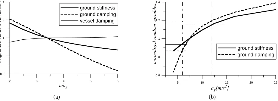
In figure 3b the integrand function in the risk estimation (12) is depicted, allowing for a visual appreciation of the PGA range (6 to 13 m/s2) mostly contributing to the failure probability. In figure 4a, the values of the random values at the design points are plotted for a conveniently larger amplification range, showing the negligible, and somehow ambiguous, effect of the vessel damping. For the same failure acceleration value a_f , in figure 4b the RVs at the design point are directly plotted as functions of the pga

According to this investigation and given the very low sensitivity of the probability of failure to the vessel damping the following criteria were adopted for refining of the Response Surfaces: (1) the random variable describing the vessel damping has been eliminated from the analysis; (2) the initial experimental points of the factorial design were replaced by the star points values corresponding to k = 2, thus focusing the parametric analysis on a smaller range of the RV’s, still centered on average values.

2 3 4 5 6

a/a_g 0.6 0.8 1 1.2 1.4 n o rm a li ze d r a n d o m v a ri a b le s ground stiffness ground damping vessel damping (a)

5 10 15 20 25

a_g[m/s2] 0.6 0.8 1 1.2 1.4 n o rm a li ze d r a n d o m v a ri a b le s ground stiffness ground damping (b)

Figure 4. Fragility refinement: RVs at design point vs dynamic amplification (a) and pga (b)

From the results of these experiments updated Response Surfaces were obtained and the new fragility curve (figure 2) was computed both by FORM and by MCS. Variance of the error for the predicted responses at the initial experimental design and at the first iteration pointed out an improvement in the fitting, with the error variance for the mean model decreasing from 0.088 to 0.071.

5 ISOLATED BUILDING (NON-LINEAR): CRITERIA FOR FRAGILITY ANALYSIS

For the case of a building resting on a isolation system based on the introduction of HDRB devices the following overall procedure is proposed, based on experimental and numerical activity, for the evaluation of the seismic fragility of the isolators.

1. Performance of experimental tests of the behaviour of the adopted HDRB devices under imposed cyclic relative displacements and constant axial force, carried on up to the specimen failure. Based on preliminary evaluation of the seismic response of the isolated building (Perotti et al, 2009) it could be recommended to run the tests for three values of the axial force, i.e. the static load in normal operation, zero load and twice the above static load. Note that the last two values can be roughly assumed as the minimum and maximum vertical load attained during the SSE seismic response.

2. Development of a refined Finite Element model of the adopted isolator, taking account of all sources of mechanical and geometrical non-linearities; the model, after a validation with respect to the experimental results obtained in step 1, is to be used to simulate a variety of additional tests, taking account of 2-D horizontal relative displacements and variable axial load.

et al (2004), is under development; validation will be again pursued according to results of FE modelling in step 2.

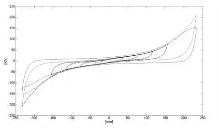
Figure 5. Isolator model: comparison of experimental (continuous line) and numerical (dotted line) experimental behaviour.

4. Statement of the limit state condition for the isolator (see the parallel paper by Corradi et al, 2009) expressing the interaction between horizontal and vertical load at failure; this activity will be supported by analytical development, by the experimental testing in step 1 and by the numerical FE computations in step 2.

5. Performance of the fragility analysis for the isolating system, according to the procedure summarized in section 3; in the development, both the limit state condition for the HDRB device as developed at step 4 and the simpler failure condition in terms of relative displacement will be introduced for comparison. In the dynamic analyses a simple rigid-body model will be assumed for the building, while the model by Abe et al (2004) will be adopted, with some modification, for the isolator behaviour.

6 CONCLUSION

A procedure for computing seismic fragilities of equipment or structural components in NPP buildings have been developed and tested.The example of application here shown, though considering a limited number of variables, demonstrates the applicability of the procedure to a real-life case.

The case of base-isolated buildings has been also treated with reference to the preliminary design of the IRIS NSSS building, based on the introduction of HDRB devices. Given the efficiency of the isolation system in reducing the seismic accelerations inside the building, the isolator itself has been assumed as the most critical component in terms of seismic risk. An overall procedure for the assessment of the fragility of the isolation devices has been summarized, based on both experimental and numerical activity.

Acknowledgements. The authors gratefully thank Giorgio Bianchi and Davide Mantegazza for their

Figure 6. Isolator model: hysteretic behaviour under SSE seismic input.

REFERENCES

Abe, M., Yoshida, J., Fujino, Y. 2004. Multiaxial Behaviors of Laminated Rubber Bearings and Their Modeling. II: Modeling”, ASCE Journal of Structural Engineering, 130:8, P. 1133-1144.

Bianchi, G., Mantegazza, D.C., Perotti, F. 2007. Dynamic modelling for the assessment of seismic fragility of NPP components. Proc. of SMiRT 19, Toronto, Canada, August 12-17.

Carelli, M.D. et al 2004. The Design and Safety Features of the IRIS Reactor, Nucl. Eng. Des., 230, P. 151-167.

Casciati, F. and Faravelli, L. 1991. Fragility analysis of complex structural systems. Research Studies Press Ltd., Taunton, Somerset, England, P. 305-355.

CEN, 2005. Eurocode 8, Design of structures for earthquake resistance - Part 1. General rules, seismic actions and rules for buildings. EN 1998-1: 2005.

Corradi, L., Domaneschi, M. and Guiducci, C. 2009. Assessing the reliability of seismic base isolators for innovative power plant proposals, Proc. of SMiRT 20, Helsinki, Finland, August 9-14.

De Grandis, S., Domaneschi, M. Perotti, F. 2008. The computation of seismic fragility of equipment components in nuclear power plant, Proc. of 4th Europ. Conf. on Structural Control, September 8-12, San Petersburg - Russia.

Der Kiureghian, A. 2005. Non-ergodicity and PEER’s framework formula, Earth. Eng. Struct. Dyn. 34, P. 1643-1652.

Faravelli, L. 1989. Response surface approach for reliability analysis. ASCE J. of Eng. Mech. 115, P. 2763-2781.

Maioli, A. et al 2005. Risk-Informed Design Process of the IRIS Reactor, Proc. of ANS PSA’05 Conference, San Francisco, September 11-15, paper 138095.

Perotti, F. et al. 2009. Seismic Isolation of the IRIS NSSS Building, Proc. of SMiRT 20, Helsinki, Finland, August 9-14.

Nusbaumer, O. 2005. Analytic Solution of Seismic Probabilistic Risk Assessment, Proc. ESREL Conf.