A METHODOLOGY FOR A SIMPLIFIED THERMO-MECHANICAL
WELDING SIMULATION IN AN ENGINEERING FRAMEWORK.
F.Rossillon1, L. Depradeux2
1EDF SEPTEN, 12-14 av. Dutrievoz, Villeurbanne, FRANCE
2EC2-MS, 66 bd Niels Bohr, Villeurbanne, FRANCE
E-mail of corresponding author: frederique.rossillon @edf.fr, [email protected]
ABSTRACT
The integrity of structures in nuclear power plants and in particular the primary components of PWRs, has to be assessed to meet given safety criteria. Following indications of Stress Corrosion Cracking (SCC), enhanced mechanical studies have been carried out to improve the knowledge of the in-service loading. For a better assessment of the mechanical state, the manufacturing process consequences have to be investigated, such as the welding operation. To fulfill this goal, numerical simulation has become a highly effective tool and an attractive alternative to measurements, in order to compute the complex loading history resulting from the welding. However, it remains a difficult task to take into account the multipass welding with a high number of beads for engineering studies with a reasonable computation time. This paper deals with a methodology of a simplified modeling of the welding: the simulation of macrobeads, by merging passes together, leads to a reduction in the model size and then in the computation time. This method enables us to have a 3D thermo-mechanical model and still ensures a good description of the mechanical state.
A steam generator divider plate is set as an application example. At first, a 2D multipass welding model is computed to have a fine description of the mechanical state. A set of “mechanical indicators” is then defined, and leads to the definition of a reference state. Afterwards, different single passes are merged in 3D macrobead and the heat input calibration is fitted to match multipass computation. The “mechanical indicators” comparison enables us to trust in the mechanical field description. The subsequent stages of the manufacturing process and the in-service load stage are then computed on the 3D model. At each step, the evolution of the mechanical variables is analysed: residual stresses, plastic deformations and hardening.
INTRODUCTION
For Nickel based alloys components of PWR, degradation mechanisms like Stress Corrosion Cracking are a major concern, especially in the vicinity of welded areas, where SCC is likely to occur. In order to prevent SCC damage or predict the evolution of potential indications, it is necessary to improve the knowledge of the in-service load in the welded zones. For this purpose, numerical simulation has become a highly effective tool and an attractive alternative to measurements. Nevertheless, it remains a difficult task since in-service load results from the complex thermo-mecanical history of all stages of the manufacturing process, including welding, post-weld heat treatment, hydro-test and transient loading of the component. Some of the stages of the manufacturing process are not straightforward to simulate, especially the welding operation, usually involving a large number of passes for such component. In the past decade, many FE models have been developed to compute welding residual stress fields for welded structures in nuclear power plants [1], [2], [3]. However, fully three-dimensional numerical simulations of welding are often devoted to instrumented mock-up [4], [5] or international round robin [8]. They are seldom initiated for industrial components in an engineering framework due to the computing time and lack of input data.
This paper proposes a simple methodology mean to compute the in-service loads on 3D geometry, taking into account the welding and the post-welding stages. First, the basics of the methodology are described. Then, a 900 MW steam generator divider plate is set as an application example.
DESCRIPTION OF THE METHODOLOGY
compared to the experimental one. In case of good agreement of the results, the model enables the assessment of the residual stress field within this specific application range. This procedure corresponds currently to the best practice but is not always suitable for an industrial purpose.
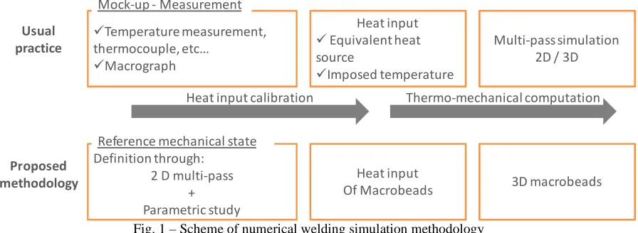
The industrial concern is to understand the in-service loading on the real 3D geometry of the component. Thus, the welding process has to be computed on a 3D-finite element model. Due to the computation time, it is not feasible to take into account individually each weld deposit. In fact, the number of passes is very high for primary PWR components and consequently the size of the model would be too high. In order to reduce the model size, the principle consists in modeling macro-beads by merging passes together. The aim is to reproduce a mechanical state after welding, set as a reference, on the 3D geometry by a simplified thermo-mechanical history. In practice, this reference enables the heat input fitting of the macro-beads of the 3D-simulation (see fig.1)
Temperature measurement, thermocouple, etc…
Macrograph
Mock-up - Measurement
Heat input
Equivalent heat source
Imposed temperature
Multi-pass simulation 2D / 3D
Definition through: 2 D multi-pass
+ Parametric study Reference mechanical state
Heat input
Of Macrobeads 3D macrobeads
Heat input calibration Thermo-mechanical computation
Usual practice
Proposed methodology
Fig. 1 – Scheme of numerical welding simulation methodology
For industrial cases, components are already manufactured and there is a lack of input data: the exact number of beads and the arrangement are not always indicated. In some special cases, measurements are available such as residual stress measurement. In our approach, as there are no measurements, the reference mechanical stage is defined thanks to 2D multipass simulation coupled with parametric study (Fig. 1). To ensure a rational heat input calibration, a set of “mechanical indicators” is defined in order to ensure an efficient reproduction of the reference state.
Mechanical indicators definition
The methodology considers FE numerical simulation so as to predict the evolution of different mechanical parameters from the welding stage to the in-service mechanical state. At first, different mechanical parameters are selected, that may vary with the objectives of the investigations. For components of PWR made of Nickel based alloy 600, SCC is the major concern. As a consequence, the residual stresses near the surface are of primary interest. However, plastic deformation and hardening are also of interest, as they constitute relevant parameter of SCC propagation [9], [10]. Following these considerations, a set of mechanical indicators are selected:
• Dimension of the zone exceeding the yield stress of the base metal during welding, and during the
hydro-test
• Maximal longitudinal (parallel to the weld direction) and transverse (perpendicular to the weld direction)
stress at the surface of the weld deposit, and at the surface of the base metal
• Maximal Von Mises stress at the surface of the base metal and weld deposit, signed with the sign of tr[σ] :
× s s
Tr
sign :
2 3 )) (
( σ with s the deviator of the stress tensor (1)
• Maximal cumulated plastic strain at the surface and of the base metal and weld deposit. This scalar
parameter is representative of the hardening of the material and is defined by:
And (2)
∫
=
t p eq peq
dt
0
.
ε
ε
&
pij p ij p
eq
p
ε
ε
ε
&
&
&
.
&
3
2
This set of indicators is computed at each stage of the manufacturing process. The analysis is completed with qualitative observations of stress and strain fields at each step of the simulation.
Welding stage simulation
Merging passes requires fitting the heat input that is prescribed in the 3D-simulation, which is not straightforward since no measurement is available. To challenge this lack of data, and to define a reference welding residual state that may be used for the heat input fitting of the 3D macro-beads model, a 2D numerical simulation of a transverse cross-section is therefore performed as a first step.
The 2D hypothesis allows the simulation of the deposit of each bead individually, given a weld-sequence. For each pass, it is therefore possible in the 2D multi-pass model to adjust realistically, if not very accurately, the heat input directly from the welding parameters, considering standard weld efficiency. Knowing the heat input for each pass, it is possible to perform the numerical simulation of welding on the 2D model by solving the non-linear uncoupled thermal and mechanical problem, with now classical FE methods [6], [7].
The residual mechanical state after welding on the 2D model is characterized by the values of the computed indicators defined above. It can be regarded as a reference state, which has to be reproduced by the 3D macro-bead simulation. The next step is the heat input fitting in the macro-beads, merging passes together, in order to match the results from the 2D reference state. On the 3D model, each macro-bead is calculated with the same FE method as a single pass of the 2D multi-pass model.
It is obvious that in such a fitting, some indicators in the 3D model are likely to be more accurately reproduced than some others. For example, by definition, the cumulated plastic strain computed with a 3D macro-beads problem might not be the same as for the multi-pass model. In fact, there are fewer thermal cycles induced by macro-bead modeling, so the global hardening is less severe. The criteria which ensure a good fitting may vary in accordance with the objective of the computation. In this paper, as SCC is concerned, the maximal stress value at the surface seems to be a relevant parameter.
Another advantage of the preliminary 2D computation is to perform parametric analysis. This enables to estimate the variability of each indicator. For instance, the effect of the pass sequence deposition upon stress indicators is investigated. As this parameter is generally unknown for existing welds, it is of importance to investigate the inherent discrepancy of welding process.
Post weld indicators evaluation
Once the residual mechanical state has been obtained on the 3D model, and validated from the 2D multipass via the indicators values comparison, the simulation of the post-weld heat treatment, and of the thermo-mechanical transient loading, including the hydro-test, has to be conducted. The indicators values are computed at each loading step. It enables to analyze the influence of the post-weld loading on the residual stress-strain field redistribution. Further investigations can also be conducted on the influence of material properties of the different part of the component.
APPLICATION OF THE METHODOLOGY TO A STEAM GENERATOR DIVIDER PLATE
This methodology has been applied to evaluate the mechanical state in the welded areas of nickel based-alloy divider plates of steam generators. Following the SCC field experience of 900MWe steam generator, the simulations are focusing to the weld between the divider plate and its stub runner, which is not post-weld heat treated.
Zone description
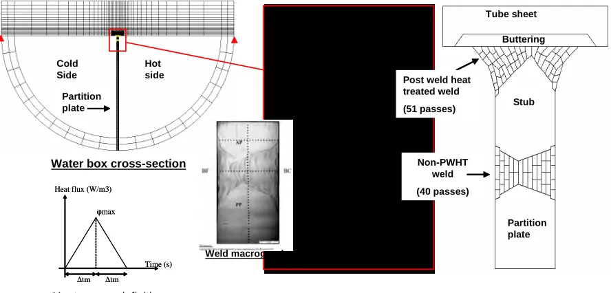
The steam generator divider plate (34mm thick) and partition stub (Fig. 2) are made of Inconel 600 alloy. They are manually welded with coated electrode, using Inconel 182 filler material. Two welds are heat treated: the weld between the stub and the tube sheet and this between the divider plate and the bottom of the water box. However, the welding of the divider plate with the stub is not subjected to heat treatment.
Fig. 2 – 3D-mesh of the Water box of a steam generator with the Nickel based alloy divider plate
2D numerical simulation of the welding
At first, a 2D numerical simulation is carried out, considering a weld cross section including the divider plate, the stub, the surrounding tube sheet and the bowl. The welding of each groove is completed in two main sequences, with approximately 20-25 passes in each sequence (fig. 2). Due to the component flange, the generalized plane strain condition can be assumed for the 2D model. Approaching this boundary condition, the model is 2D axisymmetric, but with an axis rejected far away from the section, with a radius very high regarding the dimension of the section, so that the curvature can be considered as zero.
The mesh and the weld details are shown in fig. 2. Each pass is computed individually and is included in the model one by one. At first, the thermal analysis is performed and the time-dependent temperature field is saved for the subsequent mechanical analysis. The transient temperature history is computed by solving the heat conduction equation, assuming temperature-dependent physical properties. The latent heat of fusion is neglected, as it has proven to have negligible effect on the result.
Stub Buttering Tube sheet
Cold Side
Hot side
Partition plate
Partition plate Water box cross-section
Weld macrograph
Post weld heat treated weld
(51 passes)
Non-PWHT weld
(40 passes)
ϕmax Heat flux (W/m3)
∆tm ∆tm
Time (s) ϕmax
Heat flux (W/m3)
∆tm ∆tm
Time (s)
Heat source definition
The heat input is modeled as an internal volumetric body heat source, prescribed in the weld deposit. This body heat source is constant in space, but vary linearly with time, in order to reproduce the approaching and moving
away of the welding torch. This representation of the heat input (fig. 3) allows calibrating the parameters ∆tm and
ϕmax, given the prescribed heat input E, as follows:
ϕmax ×∆tm × S = E = ηUI/V (3)
with U the tension, I the intensity, V the velocity of the welding torch, η an efficiency parameter depending
on the welding technology and S the cross section of the pass. The total net heat input is evaluated to 8 kJ/cm.
In this equation, a given value of ∆tm gives directly the value of ϕmax. Only one parameter, the time value
∆tm , has to be adjusted. The parameter is then fitted so as to match the shape of the melted zone. It means to obtain
a temperature at equal or exceeding the fusion temperature in the weld bead.
Despite its simplistic approach, this fitting method of the heat input for 2D models has proven to give very satisfactory results, the comparison with more refined model actually highlights the efficiency of the method. Indeed, 3D thermal modeling of a single bead, taking into account the displacement of the volumetric heat source gives very similar results. It reaches a satisfying compromise between a realistic description of the thermal field and the model refinement. It is very interesting and efficient particularly since no thermal measurement is available, which is usually the case for existing component.
For the thermal computation, radiative and convective heat losses with the environment are also taken into account. However, these parameters have a weak effect on the thermal results, as heat conduction in the pieces is the main heat exchange evolution. The weld between the stub and the tube sheet undergo a stress relieving heat treatment. This step is modelised by applying a temperature history to the whole model.
After the thermal transient computation, the mechanical analysis is performed. Indeed, the thermal history is set as an input for the thermal strain computation and for the mechanical properties which are temperature dependent. The FE model is the same for the thermal and mechanical analysis, except for the element type and boundary condition. A Von Mises elasto-plastic temperature-dependent constitutive equation, with kinematic linear hardening, has been adopted for all the materials during the welding stage. The boundary conditions are shown in fig. 2. During the heat treatment, the viscous behavior is assumed to follow a Lemaître constitutive equation at the isothermal temperature at 600°C. The creep deformation follows:
eq v
s p
σ
ε
& &2 3
=
with
n
m eq
Kp
p
=
σ
1/&
(4)The parameters 1/K, 1/n and m have been identified at 600°C from stress relaxation tests conducted on alloys 600 and 182 at this temperature.
Transverse stress
Longitudinal stress Transverse stress
Longitudinal stress
0 200 MPa 400 MPa
0 200 MPa 400 MPa
0 200 MPa 400 MPa 0 200 MPa 400 MPa
0 5% >10 %
0 5% >10 %
Von Mises Stress End of the welding of the
stub on the tube sheet
Von Mises Stress End of the PWHT
Von Mises Stress End of the welding
Cumulated plastic strain End of the welding Cumulated plastic strain
End of the welding of the stub on the tube sheet
Cumulated plastic strain End of the PWHT
a) b)
Fig. 4 Longitudinal and transverse stress evolution during welding a), and residual stresses and plastic deformations at different stages of the manufacturing process (end of stub welding, post weld heat treatment, end of the welding
of the divider plate) b)
3D macro-bead numerical simulation of welding
Once the indicators computation with the 2D multi-pass model has been achieved, a 3D FE model of the water box of the steam generator is set up. On this model, the weld between the stub and the divider plate is simplified into two macro-beads. Both macro-beads correspond to the two main sequences of filling of the groove. The thermal and mechanical modeling of each macro-bead of the 3D model is then performed following the same steps as for a single pass in the 2D-multipass analysis. The heat input is described as a body heat flux in the whole
volume of the macro-bead. Such as in the 2D analysis the same parameter ∆tm = 5sec is used. However, the ϕmax
parameter prescribed in each macro-bead is adjusted so that the computed indicators predicted by the 3D model match the reference results of the 2D model.
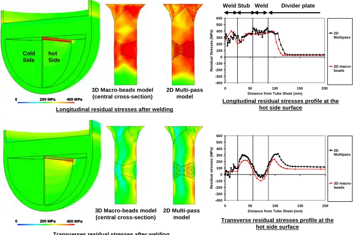
Figure 6 provides a comparison of the 2D and 3D model in the longitudinal and transverse direction. The residual stresses profile is also plotted at the surface of the warm side of the waterbox. The longitudinal stress profile is almost the same between the 2D and the 3D model: in shape and in value. On the transverse direction, the global trend along the surface is well reproduced by the 3D Macro-bead model. A difference of 100 MPa in magnitude is observed which is not very high in comparison with the variations induced by the pass order.
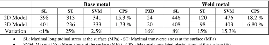
Table 1 gives the computed values of different indicators in the base metal and in the weld deposit. Except for the cumulated plastic strain which have an expected discrepancy inherent to the model, the indicator discrepancies are satisfaying: less than 25% variation. This gives a good confidence in the description of the mechanical state after welding which induce a high stress gradient.
Table 1 : Mechanical indicators values at the end of the welding, computed with the 2D and the 3D model
Base metal Weld metal
SL ST SVM CPS PZD SL ST SVM CPS
2D Model 398 313 341 15,3 % 24 446 120 476 18,2 %
3D Model 401 236 333 1,73 % 20 408 98 403 6,80 %
Variation <1% 25% 2.5% 16% 8% 15% 15,3%
• SL: Maximal longitudinal stress at the surface (MPa) - ST: Maximal transverse stress at the surface (MPa)
• SVM: Maximal Von Mises stress at the surface (MPa) - CPS : Maximal cumulated plastic strain at the surface (%)
Longitudinal residual stresses after welding
0 200 MPa 400 MPa
0 200 MPa 400 MPa
3D Macro-beads model (central cross-section)
Transverses residual stresses after welding 2D Multi-pass
model 2D Multi-pass
model 3D Macro-beads model
(central cross-section)
0 200 MPa 400 MPa
0 200 MPa 400 MPa
-400 -300 -200 -100 0 100 200 300 400 500 600
0 50 100 150 200
Distance from Tube Sheet (mm)
R e s id u a l S tr e s s e s ( M P a ) 2D Multipass 3D macro-beads -400 -300 -200 -100 0 100 200 300 400 500 600
0 50 100 150 200
Distance from Tube Sheet (mm)
R e s id u a l s tr e s s e s ( M P a ) 2D Multipass 3D macro-beads
WeldStub Weld Divider plate
Cold Side
hot Side
Longitudinal residual stresses profile at the hot side surface
Transverse residual stresses profile at the hot side surface
Fig. 5 Comparison of the results from the 3D macro-beads and 2D multi-pass model at the end of the welding
After the computation of the mechanical state resulting from the welding, the transient thermal and mechanical loading corresponding to the first hydro-test and the in-service load are computed on the 3D model. The evolution of some indicators, respectively the maximum transverse stress and cumulated plastic strain, are given as an illustration in fig. 8. The influence of the first hydro test on the global hardening of the stub level is clearly underlined. The plastic deformation of the stub increased from 1,5 % after the welding to 3% after the hydro-test. It reveals an increase of the stub hardening of approximately 1,5%. As a result, compressive residual stresses are generated at the surface in the transverse direction after the hydro-test, despite having already induced tensile stress by welding. During the in-service state, however, the internal pressure leads again to tensile stresses. Following the same methodology, computations on different SG configuration have been performed. The plastic deformation of the stub during the first hydro-test is highlighted by the yield strength difference between the stub and the divider plate. In case of a SG with low mechanical properties for the stub and high mechanical properties for the divider
plate (average ∆YS = YS(partition plate) – YS(stub runner) ~ 200 MPa), a plastic deformation of the stub occurs
with an average strain of ~5% [11]. However, the plastic deformation of the stub induces a stress relief of the welding residual state. For some SG, the stresses at the in-service state are then quite low, whereas the plastic deformation of the stub is important.
The numerical results are in accordance with experimental observations conducted on decommissioned steam generators, showing on the one hand the global hardening of the stub due to the hydro-test, and on the other hand a local hardening at the edge of the weld in the base material [11].
-200 -100 0 100 200 300 400 M a x t ra n s v e rs e s tr e s s ( M P a ) Cold leg Warm leg END OF THE
WELDING
END OF THE HYDRO-TEST IN-SERVICE STATE 0 1 2 3 4 5 6 7 M a x c u m u la te d p la s ti c s tr a in ( % ) Cold leg Warm leg END OF THE
WELDING
END OF THE HYDRO-TEST
IN-SERVICE STATE
CONCLUSION
A method for calculating the mechanical state around the welding of nickel based alloy of primary PWR components, taking into account the manufacturing stages, has been developed. The method considers a FE simulation on a 3D model, of the whole manufacturing process including welding. The weld residual stress-strain state is computed with a macro-bead method. The heat input in the macro-beads is fitted so as to reproduce the reference values of mechanical indicators, preliminarily computed with a 2D cross-sectional simulation accounting for all the weld passes. Once the welding residual state is obtained on the 3D FE model, it is therefore possible to compute the evolution of the mechanical indicators after each loading step such as the hydro-test and the operating state.
This methodology has been used to investigate the mechanical state around the welding between the stub and the divider plate of 900 MWe steam generators. Despite no fitting experimental data have been used to adjust the simulation entries, this method has revealed to be very useful to understand the physical behavior of the welded zone during the different loading stages. This has led to a better understanding of the recent destructive and non-destructive investigations performed on decommissioned SG. Nevertheless, it is possible to use this methodology for any welded zone, without thermal of mechanical measurement, provided that the weld conditions and material data are available.
REFERENCES
[1] Brickstad, B., Josefson, B.L., “A parametric study of residual stresses in multi-pass butt-welded stainless steel pipes”, Int. J. Press. Vess. Piping 75 (1), 1998, 11–25.
[2] Gilles Ph., Pont D., Keim E., Devaux J., F”ramatome-ANP experience in numerical simulation of welding”, Revue Européenne des Eléments Finis, Vol. 13, 3-4, Hermes ed. Pp.343-375
[3] Deng D., Ogawa K., Kiyoshima S., Yanagida N, Saito K., “Prediction of residual stresses in a dissimilar metal welded pipe with considering cladding, buttering and post weld heat treatment”, Computational
Materials Science 47, 2009, 398–408
[4] Ogawa K., Deng D., Kiyoshima S., Nobuyoshi, Yanagida N, Saito K., “Investigations on welding residual stresses in penetration nozzles by means of 3D thermal elastic plastic FEM and experiment”,
Computational Materials Science 45, 2009 1031–1042
[5] Lhachemi D., Robin V., Gilles P., Mourge P., Zemmouri M., “3D simulation of a peripheral adapter J-Groove attachment weld in a vessel head”, Proceedings of the ASME, Pressure Vessel and Piping Division, 2010, July 18-22
[6] L.E Lindgren, “Finite element modeling and simulation of welding”, Part 1 to 3 : Journal of thermal
stresses, 24, 2001, Part 1 : pp.141-192, Part 2 : pp. 195-131, Part3 : pp.305-334
[7] D. Radaj, Heat Effects of Welding, “Temperature Field, Residual Stress, Distortion”, Springer-Verlag, 1992.
[8] Smith M.C., Smith A.C., “NeT bead-on-plate round robin: Comparison of residual stress predictions and measurements”, International Journal of Pressure Vessels and Piping, Volume 86, Issue 1, January 2009, 79-95
[9] Deforge D., Duisabeau L., Miloudi S., Thebault Y., Couvant T., Vaillant F., Lemaire E., “Learnings from EDF investigations on SG divider plates and vessel head nozzles - Evidence of prior deformation effect on
stress corrosion cracking”, A117T04
Fontevraud 2010
[10] Couvant T., Miloudi S., Vaillant F., Deforge D., Thebault Y., “PWSCC of steam generator divider plates in
alloy 600 : coupling field characterizations with R&D studies”, A004T04