ALTERNATIVE METHOD FOR CONVERTING SEISMIC RESPONSE
SPECTRA TO TARGET POWER SPECTRAL DENSITY
Kenneth Lanham1, Mahmoud Khoncarly2, and Luben Todorovski3 1Consulting Engineer, URS Corporation, Princeton, NJ ([email protected])
2Manager of Discipline Engineering, URS Corporation, Cleveland, OH ([email protected]) 3Consulting Engineer, URS Corporation, Princeton, NJ ([email protected])
ABSTRACT
This paper presents a method for generating target Power Spectral Density (PSD) consistent with design response spectra (RS) that is based on a deterministic process which captures the phasing of seed recorded time histories when developing target PSDs. This method is based on converting of the PSD to a time history and then converting the resulting time history to RS by incorporating extracted phasing from Fourier amplitudes of earthquake motions. The process is iterative and enables automated generation of PSDs that facilitates the process of developing input time history control motions for seismic response analyses of Nuclear Power Plants (NPPs).
The precision of this method is verified by showing that the PSD and RS generated by conventional methods match the target PSD and RS of the proposed alternative method. The sensitivity of PSDs generated from differing phasing inputs is evaluated by comparing PSD developed using this alternative method and recorded seed time histories with the target PSD of Appendix A to SRP 3.7.1 that is based on thirty artificial time histories developed from equations representing a sequence of independent realizations. The impact of using random phasing for Target PSDs in the process of generating artificial time histories in contrast to use of phasing from real seed recorded earthquakes is demonstrated.
INTRODUCTION
Acceleration time histories that fit certified seismic design response spectra (CSDRS) are required as ground motion inputs to perform soil-structure interaction (SSI) seismic response analysis of new nuclear power plants. To fit acceleration time histories, SRP 3.7.1 Option 1, Alternative 1 requires comparison of PSD of a fitted time history to a target PSD in accordance with Appendix A to SRP 3.7.1. The PSDs are generally converted from seismic seed recorded time histories developed essentially by scaling of their Fourier amplitudes. Target PSDs can be fitted consistent with the target design RS in accordance with NUREG/CR-5347 and NUREG/CR-6728 starting with a time envelope function, establishing minimum PSD requirements from several trials, and performing a randomization process for several independent realizations of time histories simulated from equations differing based on random phasing. This method is tedious to implement requiring trial and error judgment. This paper presents an alternative method that has been coded to automate the process of generating target PSDs consistent with design RS. The alternative method captures the phasing of seed recorded time histories when developing target PSDs to facilitate the process of developing input time history control motions for SSI seismic response analyses of nuclear power plants.
PROCESS
The overall process to generate PSDs consistent with target RS includes the following:
1) Using a time history as the source of phasing, compute the Fourier amplitude spectra extracting the phase angle content (i.e., phasing) associated with each frequency during a conventional conversion of the time history to a PSD.
2) Using the extracted phasing, convert a starting trial PSD shape to a trial acceleration time history, and then generate a trial RS corresponding to this trial time history.
4) Iterate steps 2 and 3 until further iterations do not significantly improve convergence of the RS. Upon convergence of the trial and target RS associated with the scaled PSD, the resulting scaled PSD approximates the target PSD.
Figure 1 shows a flow diagram of conversion of a time history to RS, and conversion of a time history to PSD using conventional techniques:
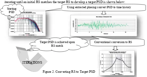
Figure 2 shows an example of an iterative process of scaling of a PSD for each realization by iterating until an initial RS matches the target RS to develop a target PSD is shown below:
FORMULATION
This section presents nomenclature and formula that was coded to automate the processes of 1) converting a time histories to Fourier amplitude spectra and then to PSDs using the FFT algorithm; and 2) reversing this process to generate a target PSDs that matches a target RS. The flowchart of Figure 4 at the end of this section provides an overview. Equations presented in this section are not derived here but are
Using extracted phasing convert PSD to time history
Conventional conversion to RS Target PSD is achieved upon
RS match
ITERATIONS Starting
PSD
Convert time history to PSD
Convert time history to RS
Figure 1. Conversion of Time History to RS and PSD
shown in summation instead of integral form as facilitated the computer program coding. The time history conversion to Fourier amplitudes can use the algorithms of either discrete Fourier transform (DFT) or fast Fourier transform (FFT). The historical advantage of the FFT, developed by Cooley and Tukey, is its increased computer run time performance due to its reduced number of operations. The approach for the FFT algorithm is to split a transform of K sample points into two K/2 point transforms.
To accurately generate Fourier amplitudes to generate a PSD per NUREG/CR-6728 requires a minimum of 100 frequency points per frequency decade. The number of frequency sample points, K, of the Fourier amplitude spectra when using a FFT equals the number of padded time steps of the time history, Np, being converted to the Fourier amplitudes. To achieve this 100 point requirement necessitates a significantly longer zero padded time history for the frequency decade ranging from 0.1 to 1 Hz. Because time history durations used in SSI analyses commonly have a duration just exceeding the minimum 20 second duration requirement of SRP 3.7.1, it is usual to extend a time history by zero padding in order to meet the 100 point per frequency decade requirement. Another benefit of zero padding for SSI analysis in the frequency domain, if the zero padding extends to approximately twice the non-zero padded time history duration, is to stop the repeating cycles of the amplitudes of the Fourier series such that they represent an ended and not a repeating pattern of continuing earthquake motion so a structural model appropriately can return to rest. In this manner the 100 point requirement is met without changing the actual time history duration. For FFT use, the number of sample points K is selected to be a power of 2 (i.e., K = 2M where M is a positive integer). For example if M = 14 and ∆ 0.005 seconds, the frequency interval is ∆ 1 2 0.005 2⁄ 0.0061 Hz with 147 sampling points in the first frequency decade from 0.1 to 100 Hz (i.e., (100-0.1)/0.0061 = 147 > 100). Consequently, a number of time steps set to this same number of 214 = 16384 frequency sampling points would zero pad a time history to a duration of (0.005)(16384) = 81.92 seconds as necessary to cover a frequency range from 0.1 Hz to 100 Hz to enable at least 100 points to be present in the first frequency decade.
Formulas presented in this section are for computing phase angles from the complex form of the Fourier amplitude spectra. A reverse option was also coded to compute Fourier amplitude spectra in complex form by combining phase angles extracted from a seed recorded time history with the absolute Fourier amplitudes from a PSD scaled to generate a resulting different time history. Conversion of this resulting different time history to a RS is also coded. The scaling factors used are derived from the compatible RS compared to a target RS. The PSD amplitudes are further adjusted during successive iterations to converge the trial RS to fit the target RS. In this manner a PSD is generated that is consistent with a target RS. The fit of the consistent RS to the target RS is not smooth as is typical of time histories fitted to RS.
The RS ratio convergence technique coded for adjustment of the PSD consist of factoring the next iteration of PSD amplitudes by the ratio of 1/(trial RS/target RS)J where J is set to 0.9 for the first iteration to facilitate more rapid convergence and where J set to 0.2 subsequently to avoid over shooting the convergence. For certain frequencies, labeled here as “dead frequencies,” the change in “trial RS/target RS” ratio does not significantly influence the PSD magnitude at that frequency, but if scaled during the many convergence iterations will unreasonably reduce the PSD magnitude at the “dead frequency”. Consequently, if the change of the previous iteration ratio of PSD magnitude at a dead frequency does not result in a significant change, then the magnitude of the final iteration of PSD at the dead frequency is set to that of its adjacent lower frequency.
The magnitude of converted Fourier amplitudes from time histories is altered by zero padding. In accordance with Parseval’s theorem the energy of the time history is equal to the energy of its converted PSD. To ensure accuracy of converted zero padded time histories and converted Fourier amplitudes, Parseval's theorem is used to scale their magnitudes:
1) To convert a time history to Fourier Amplitudes from a FFT Δ ∑
Δ ∑ | |
2) To convert Fourier Amplitudes from a FFT to a time history ΔΔ ∑∑ | |
(1)
The value of 2 used in the scale factors above is necessary to adjust for the FFT defined as a one sided Fourier amplitudes. To avoid inclusion of numerical inaccuracies during the conversion of Fourier Amplitudes to a time history it is appropriate to sum only over the actual duration of the time history and not the full zero padded length . To start the conversion of RS to PSD process, an initial PSD is read into the coded computer program that will later be scaled.
Formula:
Discrete Fourier Transform (DFT): Δ ∑ /
Inverse Discrete Fourier Transform (IDFT): Δ ∑ /
Fast Fourier Transform (FFT):
/ / /
/ /
Inverse Fast Fourier Transform (IFFT):
Δ / Δ / /
/ /
Sampling Frequency Interval: ∆
∆
Nyquist Frequency: 1 2∆⁄
Fourier Amplitude [expressed as complex number and phase angle ]:
with absolute value | | ⁄
Phase Angle: ⁄
Where | | | |
Parseval’s Theorem: Δ ∑ Δ ∑ | |
PSD for 1 sided Fourier amplitude from FFT: | ⁄|
Arias’ Intensity: ⁄ 2 ∆ ∑
Normalized Cumulative Percent of Arias’ Intensity [summed from 0 to i%]:
% 100⁄ ⁄ 2 ∆ ∑ %
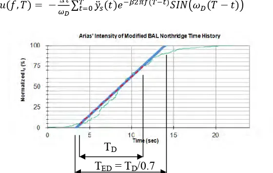
For the computation of PSD, the Fourier amplitude F(f) is summed over the total time history duration to numerically integration over the total duration instead of only the strong motion duration as defined in SRP 3.7.1 for Option 1 Alternative 1. In addition the value of strong motion duration TD in the denominator is divided by a factor FD of 0.7. This practice enables more rational generation of results beyond 24 Hz. As shown in Figure 3 the use of TED = TD/0.7 is an equivalent strong motion duration representing the effective strong motion duration based on the intersection of the sloping line with that of horizontal lines at 0% Ai and 100% Ai.
This consists of solving the equation of motion for single degree of freedom oscillators over a range of frequencies having a particular damping value subject to ground support acceleration . The
(3)
(4)
(5)
(6)
(7)
(8)
(9)
(10)
(11)
(12)
(13)
equation of motion can be written as follows to account for support motion and to reflect relative
responses . . , with mass , damping . ., 4 , and k stiffness:
This equation can be further adjusted by dividing by and substituting ⁄ and ⁄ 2 to express the equation of motion in terms of natural frequency 2 and ratio of damping :
4 2
The solution to the equation of motion for the maximum relative displacement at each oscillator frequency is the maximum of the responses at each interval of time over the duration . Duhamel’s integral also known as the convolution integral as shown below was used historically and is coded here with numerical integration to solve the above equation of motion for a damped single degree of freedom with frequency where 2 1 :
, Δ ∑ (17)
Figure 3. Equivalent Strong Motion Duration
VERIFICATION OF ALTERNATIVE METHOD
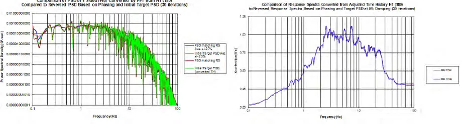
To demonstrate the capability of this alternate method to reverse the conventional process of converting time histories to PSDs by generating target PSDs to fit a RS, a time history is first converted to a RS and then a PSD and then reversed. Resulting plots are compared as shown in Figures 5, 6, and 7 of this section demonstrating close agreement.
The requirements for a compatible target PSD of the RG 1.60 spectra are published in Appendix A to SRP 3.7.1 and are based on random phasing. The use of the alternative method reported in this paper to generate PSDs to match RS also enables the study of the sensitivity of the energy distribution of PSDs generated from differing phasing inputs of various seed recorded earthquake motions because it offers a way to normalize the magnitude of PSDs while maintaining the phasing for comparison purposes. To further demonstrate the accuracy of this alternate method, time histories formed from conventional methods of scaling real seed and other wave motions are converted to RS with this alternative method and achieve a reasonably tight fit to the target RS of RG 1.60 at 5% Damping tied to a zero period acceleration (ZPA) value of 0.3g as shown in Figure 22. Figure 8 shows the resulting associated PSDs of these time histories formed from these scaled real seed and other wave motions compared to the target PSD of Appendix A to SRP 3.7.1. The 80% of target requirement of the SRP is not used to permit closer examinations. The averaged RS and averaged PSD which smoothes the responses are shown in Figures
(16)
(15)
T
D22 and 8. The averaging technique consisting of a rolling +/-20% average is also applied in separate Figures 14 and 18 to more easily view the PSDs.
The phase angles of Fourier Amplitudes associated with a time history formed form scaling the real seed Northridge earthquake with other wave motions (labeled as “No”) is shown in Figure 8 and the real seed recorded Northridge earthquake (BAL090.TH) without other wave motions is shown in Figure 9. It can be observed by comparing these phase angle plots that the phasing was altered by the conventional fitting process used to develop the time history labeled as “No”. Without the benefit of altered phasing of conventional methods that add wave motions or use wavelets, real seed recorded time histories generally do not fit well in the high frequency range above 20 hertz. In many cases this is due to the source of the motions from soil sites that have low energy in the high frequency range due to hysteretic soil damping of the response. For most cases the corrected time step published for the seed recorded time histories is 0.01 seconds which corresponds to a Nyquist frequency of 50 hertz (i.e., the maximum frequency the time history can represent). Therefore, due to the large time step, PSD responses above 50 hertz are not valid to represent the seed recorded time histories. The PSD responses are erratic below a frequency of 0.3 hertz. Therefore, review of the PSDs of seed recorded time histories presented in this paper appears to confirm the assertion of SRP 3.7.1 that “The power above 24 Hz for the target PSD is so low as to be inconsequential so that checks above 24 Hz are unnecessary”. Responses outside of this range are shown for academic interest in this paper but are not considered reliable.
FINISHED START
Read in seed recorded time history
Extract phase angles
Is iterations count met?
Read in initial PSD shape
Convert trial Fourier amplitudes and phase angles with baseline correction into trial time history Read in target RS
shape
Convert trial time history to trial RS
No Yes
Compute trial PSD energy
Compute trial TH energy
Scale trial TH using PSD/TH energy ratio of Parseval’s Theorem
Factor Fourier amplitudes for next iteration based on
target/trial RS ratio
Compute final PSD deemed to match RS Convert trial PSD to
Fourier amplitudes
Compute Arias’ Intensity including TD/0.7 ratio based on T75%-T75%
DISCUSSION OF RESULTS
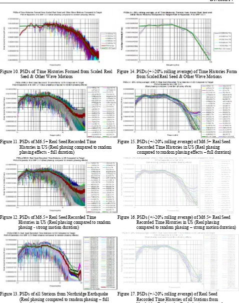
To study the effect of real phasing of seed recorded time histories compared to random phasing, two populations of seed recorded time histories are converted to PDSs for comparison of their energy distribution with that of the target PSD of Appendix A to SRP 3.7.1 using the alternate method of this paper where the time histories are altered while maintaining phasing to match the RS of RG 1.60. These comparisons are shown in Figure 11 for a sample of forty six time histories selected in the US corresponding to magnitudes in excess of 6.5. In addition, a similar comparison is shown in Figure 13 for time histories from all sixty seven stations published for the Northridge earthquake. In addition, the fitted RS associated with each of the seed recorded time histories for select US sites and Northridge earthquakes are shown in Figures 23 and 25, respectively.
Both comparisons with seed recorded time histories appear to illustrate that phasing is not random for actual earthquakes as assumed for the target PSD of Appendix A to the SRP and that the shape of an appropriate target could be significantly different for many candidate sites in the US. For the US magnitudes in excess of 6.5 shown in Figure 11, the average PSD differences with the PSD of Appendix A consist of a hump above the target PSD at certain ranges of natural frequencies from 0.2 to 0.4 hertz with a more significant gradual reduction from 3 to 30 hertz. The maximum difference in magnitude of the average of the seed PSD is approximately an order of magnitude or ten times lower than the target PSD of Appendix A at a frequency of 16 hertz. This gradual reduction is more dramatic for the PSDs of the Northridge earthquake shown in Figure 17 which appears to have very little energy in the high frequency range. Therefore, it follows that the use of the Northridge earthquake as a seed to generate a time history is a deficient choice if the interest is to capture real seed phasing in the high frequency range. By viewing Figures 15 and 17, it can be observed that the similar patterns of PSD distribution for multiple earthquakes also occur for different stations of the same Northridge earthquake. This is perhaps due to phasing being a function of the local subsurface conditions at the recording station and not a function of a particular earthquake’s magnitude.
Other observations from review of the PSD sensitivity of seed recorded time histories include: 1. The requirement for PSDs from time histories based on seed recorded time histories to be enveloped by target PSDs that are based on random phasing introduces unnecessary conservatism and thus is not appropriate. This is a direct result of their significantly differing distribution patterns. Parseval’s theorem identified that the energy of the time history is equal to that of the PSD and thus the PSD can be increased with a longer duration time history. To increase the total energy level of a PSD necessitates increase of time history accelerations or increase in time history duration to enable PSD envelope at their closes frequency point resulting in conservative excess at the other frequency points. For a more reasonable comparison, PSD and target PSD should both be based on phasing of seed recorded time histories and not the assumption of random phasing for only the target PSD.
2. The PSDs of seeds presented in this paper show wide shape or distribution of energy variations compared to the target PSD of Appendix A. Because the PSD shapes may differ for soil versus rock sites, it may be more appropriate to develop multiple target PSDs separately such as for soil, soft rock, and firm rock sites rather than over conservatively requiring all sites to each use the same target PSD.
3. The fit of time histories based on seed recorded earthquakes to RS was poor for most time histories at frequencies above 20 hertz. This appears to be related to the phasing content of the seed time histories which apparently only contain high frequency content at rock sites while other soil sites do not contain phasing to accommodate fitting of RS at frequencies above 20 hertz.
4. To produce a smoothed target PSD it would seem appropriate to average the results of multiple PSDs based on seed recorded time histories that are scaled to fit a target RS using the alternate method presented in this paper. However, as shown in Figures 19 and 20 the use of the average of the +/-20% rolling average may more easily predict a smoothed target PSD considering the number of seed recorded time histories available are limited.
differences in energy distribution compared to the use of full lengths of the seed recorded time histories. As shown in these figures the magnitude of PSDs based on 20 second middle segments of seed time histories is less than that of PSDs based on full length time histories. To more precisely develop appropriate magnitudes of PSD approximated targets for fair comparisons a method to implement the normalization of energy, mostly from the differing durations of the seed recorded time histories, is needed based on equal energy instead of equal durations of the seed recorded time histories. To save on computer program computations for artificial time histories used in linear analysis where it is practical to use shorter duration time histories, normalized or scaled PSDs to match the total energy of the target PSD, considered acceptable for design, would be appropriate as a PSD acceptance criteria to assess the energy distribution. For artificial time histories used in non-linear analysis the full time history durations of the seeds seem more appropriate so that the artificial fitted time histories reflect the magnitudes of total energy of the seeds in the PSDs converted to match the target RS.
6. Seed time histories that can be used to generate tightly fitting RS, can be identified by review of RS generated from phasing of seed recorded time histories to compare with target RS using this alternate method. It is conceivable that a tighter RS fit can be achieved by using the phasing from more than one earthquake.
Figure 5. PSD Compared to Reversed PSD Figure 6. RS Compared to Reversed RS
Figure 7. TH Compared to Reversed TH
Figure 8. Phase Angles of Fourier Amplitudes of Time History Formed from Scaled Real Seed and Other Wave Motions (No)
Figure 10. PSDs of Time Histories Formed from Scaled Real
Seed & Other Wave Motions Figure 14. PSDs (+/-20% rolling average) of Time Histories Formefrom Scaled Real Seed & Other Wave Motions
Figure 11. PSDs of M6.5+ Real Seed Recorded Time Histories in US (Real phasing compared to random phasing effects - full duration)
Figure 15. PSDs (+/-20% rolling average) of M6.5+ Real Seed Recorded Time Histories in US (Real phasing compared to random phasing effects – full duration)
Figure 12. PSDs of M6.5+ Real Seed Recorded Time Histories in US (Real phasing compared to random phasing - strong motion duration)
Figure 16. PSDs (+/-20% rolling average) of M6.5+ Real Seed Recorded Time Histories in US (Real phasing compared to random phasing – strong motion duration)
Figure 13. PSDs of all Stations from Northridge Earthquake (Real phasing compared to random phasing – full duration)
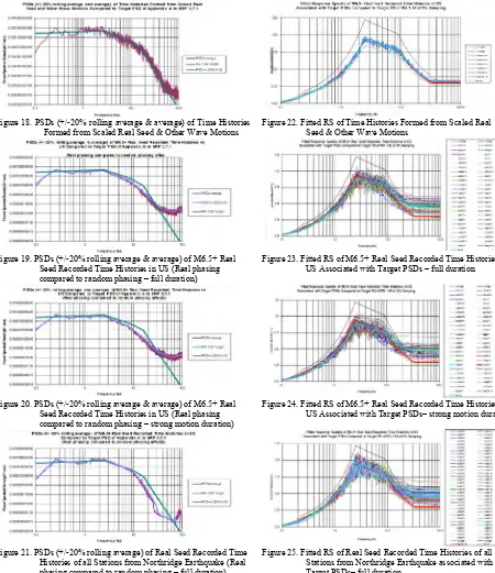
Figure 17. PSDs (+/-20% rolling average) of Real Seed Recorded Time Histories of all Stations from Northridge Earthquake (Real phasing compared to random phasing – full duration)
Figure 18. PSDs (+/-20% rolling average & average) of Time Histories Formed from Scaled Real Seed & Other Wave Motions
Figure 22. Fitted RS of Time Histories Formed from Scaled Real Seed & Other Wave Motions
Figure 19. PSDs (+/-20% rolling average & average) of M6.5+ Real Seed Recorded Time Histories in US (Real phasing compared to random phasing – full duration)
Figure 23. Fitted RS of M6.5+ Real Seed Recorded Time Histories in US Associated with Target PSDs – full duration
Figure 20. PSDs (+/-20% rolling average & average) of M6.5+ Real Seed Recorded Time Histories in US (Real phasing compared to random phasing – strong motion duration)
Figure 24. Fitted RS of M6.5+ Real Seed Recorded Time Histories in US Associated with Target PSDs– strong motion duration
Figure 21. PSDs (+/-20% rolling average) of Real Seed Recorded Time Histories of all Stations from Northridge Earthquake (Real phasing compared to random phasing – full duration)
Figure 25. Fitted RS of Real Seed Recorded Time Histories of all Stations from Northridge Earthquake associated with Target PSDs– full duration
Note: PSDs above are compared to target PSD of Appendix A to SRP 3.7.1 and RS are compared to target RS of RG 1.60 at 5% damping.
Conclusions
To study the sensitivity of real seed recorded earthquakes, the target PSD developed using this alternative method to match Regulatory Guide 1.60 from averaging of forty six seed recorded time histories selected in the US with magnitudes ≥ 6.5 is then compared to the target PSD of Appendix A to SRP 3.7.1. The Appendix A target PSD method is based on thirty artificial time histories developed from equations representing a sequence of independent realizations of variable phasing uniformly distributed between 0o and 360o established by random number. This comparison illustrates the effect of using phasing of real earthquake motions from seed recordings in contrast to use of random phasing on Target PSDs in the process of generating artificial time histories. A similar comparison was also performed from averaging of sixty seven seed recorded time histories from all Northridge earthquake stations. Both comparisons with seed recorded time histories illustrate that phasing is not random for actual earthquakes as assumed in Appendix A to the SRP and that the shape of an appropriate target could be different for many candidate sites in the US. These comparisons imply substantive impact of using random phasing for development of Target PSDs in the process of generating artificial time histories in contrast to use of phasing of real earthquake motions from seed recordings.
Nomenclature:
Acceleration time history (g) Frequency (hertz) √ 1
Number of frequency intervals corresponding to a particular frequency
Number of time intervals corresponding to a particular time Time (seconds)
Real number of real part of complex number representing Fourier amplitude
Arias’ intensity (g2-seconds)
Real number of imaginary part of complex number representing Fourier amplitude
Maximum frequency of sampling range considered (hertz) Equivalent strong motion duration factor of 0.7 with [
% %/ ]
Fourier amplitude (g) of time history as a function of frequency
Total number of frequency intervals that is the same as the total number of sampling time steps .
The power of 2 used to compute the number of sampling frequency points [ 2 ]
Total number of sampling time steps to represent the total duration of time of a time history not including zero padding Total number of sampling time steps to represent the total
duration of time of a time history including zero padding Maximum frequency that can be represented by the time history interval ∆ known as the Nyquist frequency (hertz) Power spectral density (PSD) amplitude (g2-seconds) of time
history as a function of frequency
Total time length of a time history not including zero padding (seconds)
Total time length of a time history including zero padding (seconds)
Strong motion duration % %] (seconds) Equivalent strong motion duration % %/
(seconds)
% Normalized cumulative duration as a percent of Arias intensity summed from 0 to i%
Δ Sampling frequency interval (hertz) Δ Sampling time interval (seconds)
Phase angle ranging from 0 to 360o (degrees)
References
Bathe, KJ. (1996). Finite Element Procedures, Prentice Hall, Upper Saddle River, NJ.
Design Response Spectra for Seismic Design of Nuclear Power Plants. (December 1973). United States Nuclear Regulatory Commission, Regulatory Guide 1.60, Rev. 1, U.S. Nuclear Regulatory Commission, Washington, DC.
MacLaren, L.D. and Hill, S.D. (March, 1991). A Fortran Program for Spectral Analysis using the Fast Fourier Transform, ARL-FLIGHT-MECH-TM-432 (AR-600-583) (AD-A236 848), Department of Defense, Melbourne, Victoria, Commonwealth of Australia.Seismic Design Parameters, Standard Review Plan for the Review of Safety Analysis Reports for Nuclear Power Plants. (March 2007). NUREG-0800, SRP 3.7.1, Rev. 3, U.S. Nuclear Regulatory Commission, Washington, DC. McGuire, R.K., Silva, W.J., and Costantino, C.J. (October 2001). Technical Basis for Revision of Regulatory Guidance on
Design Ground Motions: Hazard- and Risk- Consistent Ground Motion Spectra Guidelines, NUREG/CR-6728, U.S. Nuclear Regulatory Commission, Washington, DC.
Pacific Earthquake Engineering Research Center: NGA Database (1999). University of California (Regents), Berkeley, California, USA.
Philippacopoulos, A.J. (May, 1989). Recommendations for Resolution of Public Comments on USI A-40, “Seismic Design Criteria”, NUREG/CR-5347 (BNL-NUREG-52191), U.S. Nuclear Regulatory Commission, Washington, DC.