An approach towards end-to-end QoS with statistical multiplexing in ATM networks

An

Approach towards

End-to-end QoS with Statistical

Multiplexing in

ATM

Networks

S.Rampal

D. S.

Reeves

D. P. Agrawal

~enter

for Communications

and

Signal Processing

Department of Electrical

and

Computer Engineering

~orth

Carolina State University

~TR-95/2

An Approach towards End-to-end QoS with Statistical JVlultiplexing in

ATM Networks

Sanjeev Rampal, Douglas S. Reeves and Dharma P. Agrawal email: {sdrampal, reeves, dpa@eos.ncsu.edu}

Depts of Electrical and Computer Engg and Dept of Computer Science North Carolina State University, Raleigh.

Abstract

We address the problem of providing quality-of-service (QoS) guarantees in a multiple hop packet/cell switched environment while providing high link utilization in the presence of bursty traffic. A scheme based on bandwidth and buffer reservations at the Virtual Path level is proposed for ATNI networks. This approach enables us to provide accurate end-to-end QoS guarantees while achieving high uti-lization by employing statistical multiplexing and traffic shaping of bursty traffic sources. A simple round robin scheduler is proposed for realizing this approach and is shown to be implementable using

standard ATlVi hardware viz. cell spacers. The problem of distributing the bandwidth and buffer

space assigned to a VP over its multiple hops is addressed. We prove the optimality of the approach of allowing all the end-to-end loss to occur at the first hop under some conditions and show that its performance can be bounded with respect to the optimal in other conditions. This results in an equal amount of bandwidth to a VP at each hop and essentially no queueing after the first hop. Using simu-lations, the average case performance of this approach is also found to be good. Additional simulation results are presented to evaluate the proposed approach.

1

Introduction

Broadband Integrated Services Digital Networks (BISDNs) of the near future will be based on the Asynchronous Transfer Mode (~~TM) standard. These networks are being designed to support a wide variety of traffic types including voice, video and data. These traffic types vary widely in their bandwidth requirements, and tolerance to network cell transfer delay (CTD) and average cell/packet loss probability (CLP) (i.e. Quality-oj-Serviceor QoS requirements

1).

These networks are expected to employ preventive congestion control techniques through the use of a Connection Admission Control (CAC) function which admits a new connection only

if

its specified QoS can be satisfied while continuing to meet the QoS needs of currently-admitted connections.

The problem of being able to predict the QoS that a connection (also referred to as a "call" or "virtual circuit" in this paper), will receive when admitted has proved to be a very difficult one

[1].

Statistical modeling techniques for a single ATM node have been analyzed in a number of papers [13], [23]. These include approximate formulas based on large buffer asymptotics ([10], [9]) and those based on large numbers of sources [15], [13]). However, these results normally involve some approximations and have

1In general several other parameters, such as second moments of delay and loss may also be specified as QoS metrics.

T

T

C1 ₁

..

...

1

C2 ₂

2 MUX

C3

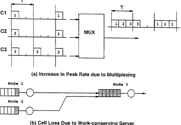
(a) Increase in Peak Rate due to MUltiplexing

Node 1 _{Node 3}

~I---_-..I:

~I---'/

(b) Cell Loss Due to Work-eonserving Server

Figure 1: Problems in determining QoS for multi-hop case

not been extended to the multiple node (end-to-end) 2 case so far. On the other hand, flow control

schemes that enable exact end-to-end QoS calculations have been proposed [12], [26], but employ peak bandwidth allocation which results in poor link utilization. This is because standard multimedia traffic

models have a peak cell rate (PCR) at least 3 to 4 times the sustainable cell rate (SCR) [29], [31].

Figure 1 illustrates the difficulty of extending admission control based on statistical multiplexing to the multi-hop case. In Figure 1a (from [17]), connection 3's minimum inter-cell arrival time changes from 3

slots to 1 slot (thereby changing its PCR), because of the work-conserving multiplexor (Note: a server is

work-conserving if it does not idle as long as there is a cell waiting far transmission). Hence in general, statistical modeling based on the traffic model at the edge of a network (which is very approximate in itself for typical multimedia sources) may not be valid after a few multiplexing and/or buffering operations. For a single node, it is intuitive that a work conserving cell transmission policy minimizes the total losses at a node. However, figure 1b shows that in a tandem queuing environment, we can encounter cell loss because of a work-conserving cell transmission policy. In the figure node 1 and node 2 both transmit a cell to node 3 which has a full buffer, leading to cell loss. This cell loss could have been avoided by the use of feedback between adjacent nodes or by the use of a nan-work-conserving cell service policy. Hence it is no longer optimal to be work conserving in order to minimize the total losses at the network level. Feedback- based schemes will be used to a limited extent in the high-speed network environment

mainly because of the high delay-bandwidth product and low loss requirements. The AT1v1 forum is

moving towards rate-based flow control techniques as opposed to credit-based approaches. We note that in general, combinations of preventive and reactive congestion control mechanisms have been found to be effective in providing network level congestion control [28]. An approach has also been investigated in which the performance (delay) achieved at an upstream node is added to a packet as it traverses a network, which is used to determine its transmission priority at a downstream node [6]. The use of

the EF?I

(~xplicit ~orward

Congestion Indication) feature in ATM has also been explored in spreading congestion information over different nodes [22]. While all these schemes indicate improved network

perf~rmanceunder certain simulation conditions, no schemes exist as yet which provide provable and predictable end-to-end QoS., along with high utilization for bursty traffic.

Cruz [7] has shown that with simple work-conserving FIFO, as loss tolerance approaches 0, the

down-stream buffer requirement grows exponentially with the number of hops

(H)

in the path. Equivalently,

if we use smaller buffers, we may have to allocate more than the peak bandwidth to ensure zero loss. In comparison, the use of a non-work-conserving scheduler can always guarantee zero losses, while requiring

only O(H) buffer requirements and peak bandwidth allocation [12]. Hence,

The optimal cell service policy to achieve a given loss specification at the network level is a non-work-conserving policy.

A hotly debated issue in the ATIvr community is the use of end-point versus hop-by-hop flow control. Again Figure 1b shows that end-point controls may be insufficient in controlling network level

perfor-mance particularly when allowable loss probabilities are as low as 10-6 _{to 10-}10 _{(TIle loss of a cell in}

Fig 1 could have been avoided if there was some feedback indicating a full buffer to the upstream nodes). In [8], DeSimone shows that traffic smoothing at the network edge alone is not sufficient in protecting a network from congestion.

In this paper, \ve propose the use of deterministic bandwidth reservations at the Virtual Path level in

order to overcome some of these problems. A deterministic cell scheduling scheme automatically results in

a hop-by-hop rate-based flow control mechanism without requiring any explicit feedback between successive nodes. This enables us to provide end-to-end QoS guarantees. Further, by employing reservations at the VP level rather than the VC level, we exploit statistical multiplexing and traffic shaping within each VP, resulting in high utilization. vVe add that in the proposed architecture, we allow for VCs to traverse more than one VP from origin to destination nodes so that in general a VC does not see a deterministic end-to-end pipe as its VP. This approach was first introduced in [30]. In this paper, a detailed description and analysis of this approach is presented.

Section 2 introduces the approach of bandwidth reservations at the path level. we demonstrate the

difficulty of the multi-hop QoS problem by presenting some important sample path properties. The

important issue of bandwidth efficiency under full sharing and partitioning techniques is also analyzed

using examples. Section 3 discusses an implementation of this scheme using round robin scheduling

and discusses other possible approaches. In section 4 we analyze the important problem of distributing

the end-to-end resources assigned to a VP over its different hops. Some important sample path and

simulation results are presented. We demonstrate the interchangeable use of bandwidths and buffer

space in order to obtain QoS and high utilizations over multiple hops. In section .5 several simulation results related to different sections of the paper are presented together. Section 6 concludes the paper and provides pointers for future work.

2

Development of a Path Level Reservation Scheme

In this section we motivate our development of a path level reservation scheme. We first examine some basic sample path properties of cell loss over multiple hops to get some insights into .the multi-.hop

QoS problem. Next we look at the traffic smoothing phenomenon and use the effective bandwidth

Q1 Q2

Arrivals at Q1

Departures from 01 (Arrivals at Q2)

Departures from 02

mu_1 lower mu_1 higher

r r

11

Figure 2: Network Loss Rate can increase if service rate of a Queue is increased

2.1

The Multiple Hop QoS Problem

We first present t\VO basic sample path results.

Theorem 1 For a single node with constant service times, and an arbitrary arrival process, if the service

rate is increased, total losses can only decrease for every sample path of the arrival process. However in case ofa network of nodes with constant service times, total losses can increase if the service rate of a

node is increased.

Proof: A sample path proof of the first part is in [32]. The second statement can be simply illustrated using an example. Fig 2 shows a two hop network with a two units of buffer space at queue 1 (including the space for the cell being served) and none at queue 2, in which overall losses increase when the service rate at queue 1 is increased.

A similar result exists for the relation between losses and buffer size.

Theorem 2 For a single node with constant service times, and any arbitrary arrival process, if the buffer

size is increased, total losses can only decrease for every sample path of the arrival process. However in case ofa network of nodes with constant service times, total losses can increase if the buffer size at a

node is increased.

Proof: A sample path proof of the first part can be found in [32]. The second part is again illustrated using an example. In figures 3 and 4, the buffer size at hop 2 is increased from 2 units to 3 units (including the space for the cell in service), but still overall losses increase for the given sample path of arrivals!

Q1 Q2 Q3

-[]o{]o-[[]o-T1=10 T2=14 T3=43

Q1

t=O

02

Arrivals at 01

Departures from 01

Arrivals at 02

Departures from Q2

Arrivals at 03

~ - Idle Server

Figure 3: Overall Losses can increase with increase in Buffer size - Part I (B1=2)

for the special case of no cross-traffic. This makes the problem of providing end-to-end QoS guarantees in

the presence of cross-traffic, approximate modeling and with the precision of the order of 10-6 _{or better,}

very difficult. These examples show that we can use more network resources (as indicated by increasing the bandwidth and buffer size) and yet end up with poorer quality of service! (as indicated by increased losses ).

2.2

Bandwidth Sharing versus Bandwidth Partitioning

Bandwidth efficiency has been mentioned as one of the main advantages of using an asynchronous trans-port mechanism such as ATM, for BISDN. However, many studies on statistical multiplexing of mul-timedia traffic models have found that full sharing is not always the most efficient way to utilize link bandwidth.

In [5], Chan and Tsang examined the bandwidth allocation problem for multimedia traffic and found that bandwidth partitioning results in better overall efficiency when multiplexing traffic classes which vary

sufficiently in their allowable cell loss (more than4orders of magnitude). Bandwidth partitioning is also

Q1 Q2 Q3

T1=10

Q1

T2=14 T3=43

Arrivals at 01

Departures from 01

t=O

02

Arrivals at 02

Departures from 02

~ - Idle Server Departures from 03

Figure 4: Overall Losses can increase with increase in Buffer Size Part II (B1==3)

the use of partitioning schemes such as time-division-multiplexing when individual source bandwidths are large compared to the link bandwidths.

Even in situations in which statistical multiplexing does yield benefits, typically, we obtain diminishing returns in terms of bandwidth savings as \ve increase the multiplexing level. Hence the loss of utilization of a partitioned scheme may be made quite small compared to a fully shared scheme if the partitioning is carried out at a sufficiently coarse level. To demonstrate this, we use an approximation based on the central limit theorem suggested in [13] for determining the bandwidth requirement of an aggregation of sources. The total bandwidth requirements for 200 voice sources based on the standard On-Off model [35] was determined with different partitioning granularities (Figure 5). The total bandwidth requirement was then determined as the sum of the bandwidths of the partitions plus the bandwidth requirement of the remaining sources which do not fall into any partition (when the number of sources per partition did not divide 200 exactly).

It can be seen that increasing the size of the partitions results in bandwidth savings initially, but once we have about 40 or 50 sources per partition, the total bandwidth requirement does not change very much. It can be seen that the bandwidth requirement for 4 partitions of 50 sources is only about 15

The studies cited above are for a single ATM node and suggest that an appropriate mix of bandwidth

sharing and bandwidth partitioning results in the highest efficiency. For the multiple node case, there are additional advantages of bandwidth partitioning as opposed to sharing .

Mean bandwidth

X106 _{Total Bandwidth Requirement of 200 Voice Sources}

81-~-""---..,....----r--...--...----r---...,..._--.--_...

7

Peak bandwidth

-6

'E

Q) E

.~5

C'"

Q)

a:

~4 x x

~_~ x x _{x x Bandwidth with Partitioning}

~3 Full Sharing Bandwidth x x x x x x x x x x x x

~ .

~

-2

10 20 30 40 50 60 70 80

Number of sources per partition

90 100

Figure .5: Illustration of diminishing returns from statistical multiplexing. Total bandwidth requirement for 200 voice sources at different partitioning levels.

expensive downstream losses. This is illustrated in Figure la where the PCR of connection 3

increased due to bandwidth sharing. Typically this occurs when a connection is multiplexed with a more bursty source .

• Deterministic bandwidth partitioning results in minimal burstiness of the output process of a given source. In [34] it is shown that the smoothing of a source is maximal when it is serviced in a uniform deterministic manner. Equivalently, in [9] De Veciana et al show that the bandwidth requirement at downstream nodes is minimized by serving a connection at precisely its effective rate (which is the minimum deterministic service rate required to meet a connection's QoS requirements). Similar results are presented in [20]. In case of a full sharing multiplexing operation, a source gets the same or more number of transmission slots as with partitioning, but these transmission slots are more random in time (depending on arrivals from other sources), so that the output is likely to be burstier than the output of the same source with bandwidth partitioning.

As another example, the squared coefficient of variation of the inter-departure times from an

M / D /1

queue can be found using Laplace transform techniques as

Cb

=

1 - p2 [32]. Modeling ATM

traffic as Markovian is inaccurate, however, this example serves to illustrate the phenomenon of

traffic smoothing. At a load of 90%,

Cb

=

0.19. Typically a

C2

of less than 0.2 is considered a

deterministic source in queueing systems. Hence this example indicates that the output process of a

M / D

/1 queue at high load closely approximates a CBR source and hence should be treated in a

synchronous manner. In section5, we present some simulations which also illustrate the smoothing

of real-life sources.

C

S1

S2~

- Keells_

~

53?

S4 Cf4

~ Kcells~

S 4 - - D J I D

~ Kcells ~

S 2 - - D J I D Cf4

<«:

~ Kcells ~

S3--DJID~

Cf

~ Kcells-..

S 1 - - D J I D

Max Delay 4K1C Max Delay KlC

Bandwidth Partitioning Bandwidth Sharing

Figure 6: Comparison of Bandwidth Partitioning and Sharing with Linear Bandwidth Allocation

simplicity of implementation and due to convenience for other network management functions such as routing and resource management [10], [23].

Figure 6 compares the bandwidth partitioning approach with the bandwidth sharing approach in the

presence of a linear bandwidth allocation scheme. For simplicity we assume we have 4 sources with the

same effective bandwidth. In the sharing scheme, the total bandwidth required for the aggregation of sources (its effective bandwidth) is the sum of the effective bandwidths of the individual sources because of the linearity of the bandwidth allocation. In the partitioning scheme too, exactly the same amount of bandwidth is required! (We assume we have some scheme such as TDTvI to perform this partitioning and are not concerned with the exact implementation at present). This is because the effective bandwidth of a source depends only on its own QoS requirements, traffic statistics and the buffer size irrespective of the number of sources sharing the buffer. Hence a linear allocation scheme such as the effective bandwidth approximation predicts an equal amount of cell loss in the two cases, vVe hence have t\VO schemes which have the same bandwidth efficiency, and result in the same ceil loss.

However, we note that in case of the partitioning scheme, queueing delay seen by each source is higher. This is because each source sees a buffer of the same size as before which is now served at a lower rate.

Typically, QoS constraints seek to limit the maximum cell delay

[27].

Hence as long as the maximum

delay is met, both schemes can support a required QoS. We can ensure this by performing the partitioning at a sufficiently coarse level that the rates assigned to each separate buffer are sufficiently high and delay stays within the specified upper bound. In any case, as we have seen earlier, we would like to perform partitioning at a sufficiently coarse level to reduce any potential loss of utilization.

We also note that buffering requirements increase with bandwidth partitioning. We wiil assume that this is not critical since given the current state of technology, buffer memory is relatively cheap. If we are able to utilize the link capacity well while providing accurate end-to-end QoS guarantees, the recurring revenues due to improved line use can be expected to more than compensate for the one-time cost of

need more buffers over the entire network.

We hence summarize our analysis of bandwidth sharing versus bandwidth partitioning in the context of QoS predictability as follows.

• At a single node with heterogeneous traffic and QoS specifications, bandwidth partitioning can lead to higher efficiency than bandwidth sharing.

• Statistical multiplexing yields diminishing bandwidth savings as the multiplexing level is increased. Hence efficiency with partitioning at a sufficiently coarse level can be made close to the optimal. Further, since non real time traffic such as file transfers can always use up unused transmission slots belonging to real-time traffic, leading to even better efficiencies. We note that non real time traffic is expected to constitute a significant portion of traffic in broadband networks. Hence with appropriate bandwidth partitioning, the utilization achieved may be very close to optimal.

• For multiple nodes, deterministic bandwidth partitioning results in minimal burstiness of the output process resulting in minimizing downstream losses.

• In the presence of a linear bandwidth allocation scheme such as the "effective bandwidth" based approaches, bandwidth partitioning results in equivalent bandwidth efficiency and minimal down-stream losses at the expense of increased delays.

• If we have only CBR sources in the network, bandwidth partitioning based on peak bandwidths can ensure no cell loss with low buffer requirements (e.g. TD:NI requires buffer space of the order of the number of sources at each hop). In contrast the buffer size required to ensure no cell loss

increases exponentially with the number of hops in a path with a full sharing FIFO scheme

[7].

• Bandwidth partitioning introduces a degree of fault tolerance (since a misbehaving source will directly affect only other sources within its own partition), and can be used to also enforce fairness for call level acceptance probabilities [29].

• Non-real-time traffic such as file transfers can always use unused slots from real-time traffic and obtain full link utilization.

Hence, if we perform bandwidth partitioning at a sufficiently coarse level that delays are satisfactory and the ratio of peR to SCR is sufficiently low, we can obtain predictable end-to-end QoS preformance along with high utilization. This motivates our development of an approach based on reservations at the VP

level.

2.3

An Architecture based on Bandwidth Reservation at the Path Level

In the earlier subsections, we have seen the relative advantages and disadvantages of bandwidth parti-tioning versus sharing with respect to achievable utilization, and end-to-end QoS predictability. Hence, we propose an architecture in which bandwidth partitioning is performed at the Virtual Path (VP) level. With appropriate VP design, we can then perform the bandwidth partitioning at a sufficiently coarse that maximum end-to-end delay requirements can be met. Since all VCs within a VP traverse the same

path, we can provide end-to-end QoS guarantees without gettin~affected by cross-tra~c. Finally, ""

VP2 Cell Loss

~--)--~(~

Hop 1

Cell Loss VP1

Hop2

VP3 VP1

Hop 1 _Hop2

Cell Loss _{Cell Loss}

Figure 7: Dealing with downstream multiplexing potential in the proposed scheme

at the VC level since we allow for statistical multiplexing of VCs within each VP. Other advantages of such an approach include simplicity of implementation and the ability to integrate call-level GoS controls in terms of call acceptance probabilities and fair network access. Some form of path level bandwidth allocation will anyway be required in order to provide call-level GaS [31].

However~ we note that in general the number of calls between a given origin destination pair may not

be large enough to drastically eliminate the burstiness of the aggregate traffic of a VP. In this case, better statistical multiplexing potential at downstream nodes may need to be exploited. In such a case in the proposed architecture, the VP is terminated at the appropriate node and a new VP comprising the aggregate traffic is started at that node. This is illustrated in Figure 7. Hence in general the configuration of VPs in the network will have to be designed in order to exploit network wide statistical multiplexing potential in the most efficient way.

3

Irrrplernerrtat ion of the Proposed Architecture

In the previous section, we have motivated the development of an approach involving deterministic bandwidth reservations at the VP level. We know suggest a simple implementation for the same.

VP bandwidth guarantees are enforced using a deterministic scheduler. In this paper we investigate

the use of a Weighted Round Robin (WRR) type scheduler (equivalent to a multi-rate time-division multiplexor). The WRR scheduler is very simple to implement and analyze. Many other deterministic schedulers, such as Earliest Due Date [11] Stop&Go [12] or Weighted Fair Queuing [26] could also be

used. However, these are significantly more complicated than WRR, and with our method vVRRis good

enough to achieve high utilizations (as we will show). We discuss the use of other schedulers briefly

towards the end of this section. The idea of round-robin type service of different traffic classes for

ATM has been suggested by others also (see Sriram's Dynamic Time Slice Scheme in particular [35]).

Input

Ports

...

• I

·

.

·

.

---+----1....

·

Non Blocking

Switch

Fabric

Output

Ports

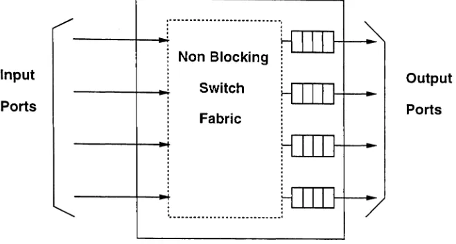
Figure 8: Model of Output Buffered ATM Switch under Consideration

particularly for the multi-hop case. Additionally, all the proposals for round robin service have employed a work conserving server in contrast to our non work conserving approach.

In this section, we assume that using a WRR server, \ve provide an equal amount of bandwidth to a VP at each physical hop. However, in general it is not clear that this is the best strategy in all cases. In section 4, we analyze this problem in detail. For now, we assume that an equal amount of bandwidth is assigned to the VP at each physical hop.

3.1

Operation of the WRR Server

We model each AT1JI switch in a path as an output-buffered multiple input multiple output switch as shown in Figure 8.

We assume that cell loss only occurs due to overflow of the output buffers and no cells are lost due to contention within the switch fabric.

Let the length of a server cycle be

T

time units (we assume the time unit is the transmission time of a

single cell). Let there be K

+

1 VPs being served by this server, denoted Vo, VI,V2 , . . .VK· Vo denotes

a VP carrying best-effort type traffic e.g. data files, network management traffic etc. Such traffic is not normally delay sensitive and we assume that provision of an appropriate long-term average bandwidth

for such traffic is sufficient. Let the number of slots reserved for Vj in each server cycle be denoted nj.

The output buffers at each port is logically partitioned such that a buffer of size BJ is reservedfor Vj

at the appropriate output buffer at the h'th switch in the path ofVj. The server cycles through all VPs

carrying guaranteed traffic (viz. VI through VK) according to a preset deterministic schedule in a strict

TDM-like manner. In each cycle, Vj is served for exactly nj slots. IfVj does not have a cell to transmit,

a cell from B_o (the best-effort queue) is transmitted instead. If Eo is also empty, no cell is transmitted

and the server is idle.

These definitions are illustrated for 4 VPs in Figure 9, where VI is assigned 2 slots, and V2 _{and V}3 _are

assigned one slot each (nl

=

2, n2

=

1,n3

=

1,

T

=

4). Va

is not assigned any slots in the cycle and only

T

VC1JL

VC2~~="··~·~~""""··""·"··"·

,"

JVTMultiPlexor

, &Shaper

~

VP2~

VP3 _ _ _

[[ITII-e

_VPO

Figure 9: Logical Model of Single Output Buffer in WRR Scheduling Model

node and itself consists of several bursty Yes. In general each VP sees a service "window" followed by

a server "vacation" while other VPs are served. '

Let d~ denote the maximum delay that can be encountered by a cell in the switch fabric of the h'th

switch in the path. We will assume that the server cycle time T is larger than this delay. Note that

typical switch fabric delays are of the order of a few microseconds at most

[27L

while the server cycle

time will be of the order of a few milliseconds as we shall show later.

Using the above notation and assuming that d~

<

T, we state the following theorem.

Theorem 3 In a network employing the vVRR scheduler described above at every node" no cell of a VP

is lost due to buffer overflow at every physical hop after the first if at at each hop h . the buffer reserved for Vj (Bj) is at least 2

*

nj cells.

Proof: The proof follows from the non work-conserving nature of the WRR server [32] o.

For simplicity, we currently assume that the server cycle is of the same length at each hop. In general, this need not be so. However, no cell loss at each hop after the first can still be ensured with appropriate buffer sizing as we show later.

3.2

A Call Admission Procedure for a VC over a Single VP

Using the above scheme, a simple call admission procedure can be used to provide an accurate end-to-end QoS guarantee for any VC traversing a given VP. We limit the term "end-to-end" to refer to the multiple hop path traversed by a single VP. As mentioned earlier, in the proposed architecture, we allow V'Cs to traverse multiple VPs. Development of admission control algorithms for VCs traversing multiple VPs is

(1)

We consider QoS guarantees of the type Prob( d,

>

D) :::;

E, where d, is the end-to-end cell delay of cells

of a connection i using the given VP (say Vj). vVe need a statistical guarantee on the end-to-end cell

delay. We convert this into two guarantees viz. a deterministic guarantee on the maximum cell delay and an average cell loss probability guarantee. Hence the cells which get lost are the only ones which fail to

meet the specified delay bound D. It can be seen that if we can bound the maximum cell delay by D

and the average cell loss probability by E, it is sufficient to guarantee that the original QoS guarantee

will also be met. Hence, this is a conservative approach to providing statistical delay guarantees.

The specified statistical delay guarantee is concerted into a deterministic guarantee on maximum delay and a guarantee on the average cell loss. This approach is sufficient (though not necessary) to meet the original QoS specification.

An upper bound on the maximum end-to-end delay experienced by any cell of Vj which traverses H

physical hops, can be easily calculated as

H

D

max ==

LBJ

InjJ

*

T

+

(BJ - LBJ

/njJ

*

nj)/C

+

2

*

(H -

1)

*

T

+

LT;op

h=l

where C is the physical link capacity (assumed same for all hops), and T;rop is the propagation delay for

the h'th hop [32].

The first two terms represent the maximum queueing delay at the first hop of the VP. When nj is small

compared to the buffer size

BJ,

this can be approximated as,

H

D

max

~

(BJ /

nj)

*

T

+

2

*

(H -

1)

*

T

+

L T;rop

h=l

(2)

Now the first term can be seen as simply the buffer size at hop 1 divided by the bandwidth reserved for

this VP (njIT), while the second term implies a constant delay of up to T at each hop after the first.

Denote by F(i,j), the CAC function used within VP Vj to admit or deny admission to requesting VC

i. The exact nature of the CAC function is not critical to our discussion. vVe assume that it determines whether the cell loss probability for i along this path will be within the user-specified allowable loss

bounds.

F

is a function of the set

Sj

of VCs currently admitted within Vj, the bandwidth

Cj

reserved

for V· the multiplexing buffer size B~ at the first hop ofVj and the QoS requirements and traffic model

of

th~'

requesting

ve.

This could

b~

based on bandwidth tables computed offline, or on approximate

formulas such as equivalent capacity [10] or any other scheme. F(i,j) results in the value TRUE if the

CLP is acceptable, otherwise it results in the value FALSE.

When a call i requests admission into VP Vj the following call admission control procedure is executed.

Compute F(i,j) and D_{m ax} (from Eqn 1). Accept the call only if F(i,j) = TRUE and Dm ax

<

D else

reject the call.

3.3

Choice of

WRR

Server Cycle Length

• Cell Transfer Delay

From Eqn 3 we note that the maximum end-to-end queueing delay increases with T and the shaping

b~ffer ~t.ho~ 1,

B}

assuming a given bandwidth assignment to this VP (which is

nj/T).

To ensure high utilization, we would like to have as large a multiplexing buffer as possible so that to ensure the end-to-end delay requirements are met, so we need a short cycle length. The 'WRR scheduler

is characterized as having the delay-bandwidth coupling problem

[1]

since a VP assigned a lower

bandwidth experiences higher network delay.

• Cell Loss Probability

Even when the bandwidth assignment to a VP is fixed (nj/T), choice ofT can affect ceil loss since

each VP sees the WRR server as an "On-Off" server with vacations. A simulation analysis of this

phenomenon is presented in section 5 which indicates that as long as T is less than a threshold,

the cell loss is relatively insensitive to the choice ofT. However, T must be below this threshold .

• Bandwidth Allocation Granularity

With a cycle of length T, the bandwidth assignments to any VP will all have to be in multiples of

the basic unit of allocation viz. liTunits. WhenT is small, this unit bandwidth can be quite large,

leading to possible loss of utilization due to quantization errors. Hence a large value of Tallows

better bandwidth allocation granularity. In their study of bandwidth quantization in BISDN [19]~

Lea and Alyatama suggest that network performance will not get severely affected if the bandwidth assignments are quantized into 10 or more levels.

• Cell Delay Variance (CDV)

Finally, delay jitter or the difference between the maximum and minimum cell delays increases with

the maximum delay i.e. withT so that small values ofT are beneficial.

In order to resolve the contradictory requirements on the value of T, a multi-level round robin may

be employed. Such a strategy was proposed in [12] as the Stop&Go strategy. The same approach can

now be employed at the VP level to tradeoff different requirements on the value of T. However the

implementation complexity of such a scheme increases dramatically with respect to a one-level scheme in that case.

As a practical guideline, we suggest the value ofT to be of the order of the propagation delays or less. This

ensures that the end-to-end delay is not dominated by the value ofT but rather the propagation delays

and the queueing delay at the first hop as seen from eqn 3. Since the propagation delays are constant and uncontrollable, the end-to-end delay can be controlled by simply the bandwidth and buffer assignment

at 110P 1. Typical propagation delays for WANs are several milliseconds per hop. Hence a value of about

1 msec would be a good choice for the cycle length. This cycle length results in a bandwidth granularity of about 424 Kb/s which is about 1/365 times the link bandwidth so that allocation granularity appears to be sufficiently fine as per the study on bandwidth quantization in BISDN [19]. Finally, as we show in section .5, by using cell spacers at the first and last hops of every VP, we can ensure that the variance in delays over the end-to-end path as well as the cell loss probability becomes independent of the value of

T. However, much more study needs to be done on resolving the different tradeoffs involved in choosing

VP. Originating at this node

r--r--r-T-~-r--r~_ Buffer for

""'--'--...L-.I.--r...r.I--J1real-time data

c..'\.

~ R~mission

- - ' \ - POinter

Output Unk

Buffer for non real-time data

Figure 10: Use of a Cell Spacer to implement the vVRR Scheduler

3.4

Implementation of the WRR Scheme Using Cell Spacers

It has been suggested that cell spacing at each NNI in an AT:NI network can be effectively employed

to improve network link utilization

[14].

The WRR scheme suggested above can easily be implemented

using a cell spacing algorithm, so that the implementation complexity of the proposed scheme appears

to be reasonable. A cell spacer is used to enforce rates and ensures against increase in jitter

[14].

Hence

a cell spacer can also be used for strict rate enforcement as is required in the proposed scheme.

Figure 10 shows a schematic of a cell spacer similar to that in

[14].

By partitioning the output buffer,

serving this output buffer according to strict non work conserving schedule, while utilizing free slots for data from the non real time buffer, the vVRR scheduler can be implemented. vVe do not go into the hardware details of this architecture at present since our goal is simply to show that using a cell spacer and a WRR scheduler have similar implementation complexities. The two key points which must be incorporated into the spacer algorithm are the non work conserving nature of service with respect to the real-time data and use of non-real-time data in case of available transmission slots corresponding to tel-time data.

3.5

Other Relevant Issues

In this section, we briefly mention some additional relevant to the proposed approach. These issues are not analyzed in this paper.

• Different Cycle Lengths in the Network

In general, the server cycle length can be different at different switches in the network. The proposed approach can readily be implemented in such a scenario. In fact the cycle length can differ even between the different output ports of the same switch. The required buffer space to ensure no loss

upstream buffe.r of the VP. The CAC algorithm suggested above can also be easily be modified to accomodate this case. vVe do not analyze this case here.

• Statistical Multiplexing of VP Bandwidths

In the proposed approach, each VP is deterministically isolated from other VPs. However this

does n?t eliminate statistical multiplexing between VPs for call-level grade-oj-service. The VP

bandwidths can be dynamically updated according to call arrival statistics with the additional

cons~raintthat the each individual VP continues to remain a deterministic pipe and per-call QoS

contIn~es to be met for each VP. Hence, we can allow Jar call-level statistical multiplexing while

etisuruiq per-call QoSusing such an approach .

• Use of other schedulers to implement path level reservations

We have suggested the use of a simple round-robin scheduler since it is the simplest technique

for implementing bandwidth reservations. This scheduler does have its problems including the

tradeoffs involved in choosing the WRR cycle length and the delay-bandwidth coupling problem. The problem with server cycle length may be reduced by using a multiple level round-robin server

such as HRR

[16]

or Stop

&

Go

[12],

however implementation complexity increases accordingly and

an engineering decision may be required to determine the right approach. The delay-bandwidth

coupling may be eliminated by using servers such as the EDD scheduler

[11].

However, the EDD

server suffers in the presence of heterogeneous traffic in addition to having high implementation

complexity. Rampal et al,

([29],

[31]) present an evaluation of some of these schedulers.

4

The Multi-hop Bandwidth and Buffer Assignment Pr-oblem

In the above sections, we have proposed an approach based on reservation of link bandwidths and buffer

space for each VP. However, an unresolved issue is that given the total resources reserved for a VP~

how should one optimally assign these over the different physical hops of a VP. In the previous section, we have assumed that the bandwidth assigned to a VP is the same at each hop and the most of the end-to-end buffer space is assigned to hop 1 for shaping. However, this need not be true always. In this section, we will compare the performance of different multiple hop resource allocation policies (:LvIHRPs). We note that assigning different resources at different physical hops of a VP is equivalent to obtaining differing levels of QoS at each hop. Hence, the problem is equivalent to splitting the end-to-end QoS

specifications into per-hop QoS specifications

[24].

A policy which obtains the per-hop QoS specifications

given the end-to-end QoS specification will be referred to as a QoS allocation policy. In this section, we will only concern ourselves with one end- to-end QoS metric and its per-hop allocations viz. the cell loss

probability (CLP) or cell loss rate (CLR). A similar problem was also addressed by Onvural and Liu

[25].

However, in their model, the link bandwidt h was fully shared by all VPs unlike our reservations-based

approach.

Figure 11 shows a model of a VP which we use for analyzing the properties of different MHRPs.

A VP is essentially modeled as a tandem queue ofH deterministic servers. There is no cross traffic and

external cells enter only the first queue and depart from the last. The buffer space reserved at hop h is

Bh and the service rate at hop h is

c-.

Note that this model is consistent with our approach of complete

• ••

Figure 11: Model of VP Traversing H Hops

We first define the MGF (Maximal Gain First) QoS allocation policy as follows.

Definition

1 Maximal Gain First Policy: The Maximal Gain First policy allots the entire end-to-end loss to the first physical hop of a VP. Transmission at all further downstream hops is required to be loss-less.

Note that in order to analyze the cell loss with an MGF allocation, we only need to look at hop 1since

no cell loss occurs at downstream hops.

Theorem 4 states that in order to implement the MGF policy, we must keep the service rate of all servers in the path at least as much as the rate at the first hop. Note that this is equivalent to to having the bandwidth at each hop at least as much as that at hop 1.

Theorem 4 To ensure no cell loss at all hops after the first, for any arbitrary arrival process, the service

rate of each server must be at least as much as that at the first hop. (i.e.

C

1 :::; C'", h == 2,3, ... H ).

Proof: The proof is in [33].

We now analyze the performance of the JvIGF policy wrt other l\IIHRP policies.

4.1

Simultaneous Bandwidth and Buffer Assignment

Consider the problem where we are given the total amount of end-to-end buffer space B and the service

rate at the last hop (CH) and are required to find the per-hop buffer and service rate assignments in

order to meet a specified end-to-end loss rate L.

Theorem .5 states that an MGF type allocation with all service rates equal to that at the last hop and the entire buffer space at hop 1 results in the minimal number of cells lost for any sample path of arrivals as compared to any other service rate and buffer assignment with the given constraints.

Theorem 5 Given the total amount of end-to-end buffer space B and the service 'rate at hop H (CH ) ,

an MGF type configuration with Bl == B, B2 _{== B}3

= .·.

₌₌

BH ==

a

and

C

1 ₌₌

C

2

= ... =

_CH _{results in}

the minimal number of losses for all possible sample paths of arrivals.

Proof: The proof is in [33].

fu~

,freedom to allot the per hop buffers with a given sevice rate at hop H, the MGF policy results in minimal end-to-end loss.

Hence,

Cor?llary 1 Given the end-to-end buffer space and service rate at hop H, the iVIGF policy with equal

service rates at each hop and the entire buffer space at hop 1 is the optimal policy for achieving a given

end-to-end loss specification.

This is because, since the :N1GF configuration achieves minimal losses for all possible sample paths of arrivals, if a given end-to-end loss specification is achievable at all by any policy, then it is certainly achievable by the :N1 GF policy as well.

Theorem 6 uses the above theorem to state that the :NIGF policy results in the minimal total bandwidth (sum of the service rates over the path) required to achieve a given end-to-end loss specification.

Theorem 6 Given the end-to-end buffer space B, the J11GF policy with equal service rates at all hops

and the entire buffer space at hop 1results in the minimal total end-to-end bandwidth required to support a given end-to-end loss rate. Further, the bandwidth requirement at any hop with the JvIGF policy is never more than the bandwidth requirement at the corresponding hop under any other multi hop resource allocation policy.

Proof: The proof is in [33].

This theorem states that not only is the total end-to-end bandwidth requirement minimized by using the :NIGF policy, but also the bandwidth at each hop is also minimized. In other words if \ve have another MHRP which results in the same end-to-end losses for any sample path, then with the IvIGF policy can achieve the same number of losses with a smaller total bandwidth requirement. Also the bandwidth requirement with the :NIGF policy will be smaller at each hop as compared to the other assignment. This is a very strong result and is a direct consequence of the optimality of the J\tIGF policy in minimizing end-to-end losses.

Finally, the optimality of the MGF policy can be extended to the network level. Consider a network with several VPs in which there is no statistical multiplexing across VPs (as in our scheme).

Corollary 2 In anetwork with no statistical multiplexing across VPs, given routing of VPs, by employing

the MGF policy within each VP, we obtain the maximal value of available bandwidth at each link of the network. This also results in minimal value of the sum of the bandwidth requirements over all VPs in the network.

The above corollary is a direct consequence of the fact that by employing the :NIGF policy within each

VP we obtain the minimal bandwidth requirement for each VP at each hop in its path.

,

The results stated above show that when we are given the total amount of VP buffer space, using the entire buffer space at the first physical hop of the VP and an equal amount of bandwidth at each hop results in the maximal utilization of each link of a network while satisfying the end-to-end loss

4.2

VP Bandwidth Allocation with Fixed Buffers

In general, buffer space assigned to a VP may not be moved around between different hops as required by the above results. Hence, we now consider a situation where buffer space is reserved for a VP at each hop but unused buffer space at one hop cannot be utilized at another hop.

In this context, we will implement the MGF policy with equal service rates at each hop. Clearly, the buffer space at downstream hops is wasted by the MGF policy so that it is not optimal. However, we show that the bandwidth requirement using the MGF policy is still within an easily computable constant

factor of the optimal assignment.

We assume that the required service rate at hop 1 with the MGF policy is calculated using an effective bandwidth function [13] or offline computed bandwidth versus loss tables. For a given source, the effective bandwidth depends on the buffer size and the required loss rate. Let T

Bl (p)denote the effective bandwidth function as a function of the loss rate. Since the MGF policy allots the entire loss to hop 1, clearly the bandwidth requirement at each hop with the MGF policy is T_Bl (L ) where L is the specified

end-to-end loss rate. vVe assume that the arrival process has a steady state mean rate and that the loss rate is sufficiently small that the steady state mean rate at the input is approximately the same as the steady state mean rate at the output. Let R denote the ratio of TBl (L ) with this mean rate. Then, the

following theorem bounds the total bandwidth requirement of the MGFpolicy with the optimal under

the fixed buffers condition.

Theorem 7 With a fixed per-hop buffer assignments, for a given end-to-end loss rate the total bandwidth

requirement with the f\;lGF policy is no more than

R:ff-l

times the requirement with an optimal policy which results in the 'minimal total bandwidth. (R is defined above and H is the number of hops in the path.

Proof: The proof essentially exploits the monotonic relation between service rate and loss rate (Theorem1)

and is in [33].

As an example with

R

= 2 over a 4 hop path, the total VP bandwidth with the rvIGF policy is n omore

than 1.6 times the optimal. In practice, we can expect the IvIGF policy to perform much better than

the above worst case bound, however, this bound enables a quick estimate of the bandwidth requirement of the MGF policy wrt the optimal. Actually finding the optimal configuration may prove to be quite difficult as the simple examples in section 2 have shown.

An approximation commonly made in practice is that traffic characteristics are unaltered as we move from one hop to the next [18]. Simulations under certain conditions indicated this assumption is approximately correct in a full sharing environment in which the bandwidths of individual sources are small compared to the link rate. With this approximation, the relationship between bandwidth and loss is unchanged over different hops, so that the same effective bandwidth function can be used for bandwidth allocation at different hops. Under our scheme of bandwidth reservations, this assumption is not quite valid. However, proposition 1 shows that if for practical reasons, this assumption is in fact made, then the MGF policy can be sown to be optimal even in the fixed buffers case. Also, since the effective bandwidth function depends on the buffer size at each hop, for this result, we assume that the buffer space at each hop is the same.

results in the minimum value of total VP bandwidth as compared to any other policy which achieves the same end-to-end loss for the same sample path of arrivals (which can be arbitrary).

Proposition 1 suggests that the MGF policy is once again optimal with equal buffers at each hop and if

we

~ake

the

ap.proxi~ation

of using the same effective bandwidth function at each hop. In the following section, some simulation results are presented which indicate that even with fixed buffer allocation the

perfor~ance

of the MGF policy is better than most other allocation policies. This is because by alloting

the entire loss at hop 1~ we are able to extract a high bandwidth reduction, while if »relet some loss

occur at downstream hops, it becomes progressively more difficult to extract bandwidth reduction. In any case, estimating effective bandwidth at downstream hops becomes difficult and more approximate because traffic characterization at downstream hops is very difficult.

In general though, we may have very large downstream buffers because of which, it may make more sense to experience cell loss downstream. In [32], we present a heuristic which assigns all the available cell loss to a downstream node and peak bandwidths at all hops preceding this hop. This ensures that the traffic model at the network edge can also be used at the downstream node, while obtaining performance which is provably better than the MGF policy.

5

Sirnulat ion Results

In this section, we present a number of simulation results which support some of the arguments made in the earlier sections.

5.1

Multiplexing Potential of Real-life Sources

We first present some plots of bandwidth requirements for real-life sources, which indicate that signifi-cantly high utilizations can be achieved with a single multiplexing operation, so that the output can be treated as a CBR process requiring a deterministic bandwidth reservation.

Figures 12 and 13 show the per-source effective bandwidth requirement for a multiplexed set of voice

sources and a multiplexed set of video sources, respectively. These curves are obtained by using the

equivalent bandwidth approximation [13], [10]. The delay shown in the curves is the maximum queuing delay that would be encountered in the first hop of the VP onto which the sources are multiplexed. The standard On-Off model with exponentially distributed On and Off durations was used for the voice sources [35]. The video model used was a well-known Markov-modulated fluid model with 11 states [21].

From this curve the multiplexing potential of both video and voice sources can be clearly seen. For

example, for 20 voice sources and an allowable queuing delay of 100 msecs the per-source effective rate is

about 16 Kb/«:this represents an average utilization of 70%. For 20 video sources and an allowable delay

Per-source Effective bandwidth (std voice model, 5% loss)

1 source

10 sources 20 sources 50 sources 100 sources

\ ".

\ "..

1.6 \

\

,

1.4 \_,

100 200 300 400 500

Shaper delay (msecs)

600 700 800

Figure 12: Per-Source Effective Bandwidth Requirement for Multiplexed Voice Sources (Fluid-flow model, peak 32Kb/s, mean 11.24 Kb/s)

Per-Source Effective Bandwidth for Multiplexed Video Sources

X106

11r----~---_r__--~---_r__--__r_---r__--_...

5

,_, ,

, ,_, "

" "

...

....

N=1

N=10

N=20

N=50

N=100

140 120

100

60 80

Shaper delay (msecs) 40

20

4l-_ _

--L..---.l---L...---.L---'----.&---o

5.2

Effect of WRR Cycle length on Cell Loss Probability

In this section we present some simulation results on the variation of cell loss probability with the cycle length of the WRR server.

The simulation is simplified by two observations. Due to the fact that VP bandwidths are guaranteed, we can safely analyze a single VP in isolation (Le., without considering influence of other VPs). Also,

since losses occur only at the first hop, we need only analyze the losses at the multiplexing buffer

BJ

of

Vj to measure the end-to-end VP loss.

We simulated a single VP Vj, which was deterministically guaranteed a bandwidth ofC'j bits/sec using a

WRR server as described earlier. We denote byTon andTof f the On and Off periods of the vVRR server as

seen by Vj; the server period is T

==

Ton+Toff. Note thatC'j = C*Ton/(Ton+Toff)

==

C/(l+Toff/Ton).

WhenTo!f andTon are varied, the bandwidth Cj remains the same if the ratio_{To! f /Ton}remains constant.

However the server "burstiness" varies as T changes. As T becomes smaller and smaller, the server

performance approaches that of a uniform deterministic server. A larger value of T results in a much

more "bursty" service, which may result in higher losses. In our description of the vVRR server earlier~

we have commented on the effect of cycle length on different QoS parameters of interest.

The voice traffic model was the same as earlier, except that cells were generated deterministically at a constant rate corresponding to 32 Kb/s during the 'ON' periods. In all cases, 1,5 voice sources were

multiplexed into a single VP of bandwidth

C

=

200Kb/s. The assumed link speed was 155 Mb

/s.

5.3

CLP Variation with Buffer Size

Figures 14, 1,5 and 16 show the variation in average CLP with the unit bandwidth of the WRR server

(i.e., 1 cell / T time units). For these experiments the multiplexing buffer size Bj was set to 10 Kb, 20

Kb and 40 Kb respectively. Note that tolerable loss probability for voice traffic is .5-10%[24].

Two distinct regions of behavior are observed. The losses vary linearly in each of these regions. For

small unit bandwidths, (large values of T) the slope is high: vVe refer to this as region 1. For large

unit bandwidths (small T), the slope is nearly zero; this is region 2. The location of the transition point

between the two regions is sensitive to the buffer size

By.

Some inferences that we can make from the

above plots are as follows.

• Let Qcycle

==

Cj

*

Ton denote the amount of data ofVj that can be transmitted by the WRR server

in one cycle. The transition point corresponds to the unit bandwidth at which Q cycle ~

BJ.

In

region 1, Qcycle

>

BJ,

and the server completely empties the buffer during .each On ~eriod. In

region 2, Q cycle

<

B},

implying that the WRR server cannot empty the entire buffer m one On

period. Once the buffer has been emptied, the remainder of the slots assigned to Vj will be wasted,

except for cells that arrive during the On time. Hence in region 1, even the average service rate

offered toVj decreases linearly with the unit bandwidth (ignoring the arrivals during the On time),

resulting in the exponential increase in cell loss.

• In region 2 CLP is nearly constant. This implies that as long as Q cycle

<

B},

the CLP is

inde-pendent of

~he

WRR cycle length. Thus the server

cycl~ lengt~

can be

~hosen

to optimize delay or

quantization effects, as long as it is short enough to satisfy this constraint on Qcycle.

o

15 sources, VP BW 200 Kb/s, Link BW 155 Mb/s, buffer 10 Kb

i. -s,

'~'8

' 0

*'

o , 0

"*...0

o ~ 0

0'*

0'

,

, 0 0 ,0 0 )IE

~ " " , 0)1\ 0 0

o "iIE 0 ')1/0 ' , 0 0 0 _~ ~

o 0

* -*-""*-

0' 0 /0

o 0 0 \ /

10°L-:---r---,---r---r---.--r----r---r---~-_.

0.2 0.4 0.6 0.8 1 1.2

Unit server bandwidth

1.4 1.6 1.8 2

x104

Figure 14: Variation of CLP with Unit Bandwidth

(BJ

10 I{b)

15 sources, VP BW 200 Kb/s, Link BW 155 Mb/s, buffer 20 Kb 10°,....----,---~--r_"---.---~--r-"---,---~--r___-~

\

\ ,0 ~

0\ \0

,

0 ' 0

'*

,

o ' , 0 0 0 0 0

)I(-*-~__~ 0 ""~... 0 0 0 0 0

o 0 0

"*

0 ...~ ~ 0 O)IE w

o ' )l(.. "'" ,....

o 0 0 y ';t(' 0 , 0 /

o " 0

o 0

o

0.2 0.4 0.6 0.8 1 1.2 1.4

Unit server bandwidth

1.6 1.8 2

x104

15 sources, VP BW 200 Kb/s, Link BW 155 Mb/s, buffer 40 Kb

o

o

o

o o

o 0 0 ",

A 0 I ,

*

o ,,*--~ I 0 , 0 0 "

"-~ '*- I 0

"-i-0

~ 0 0

"-)IE-*,

0

0 ₀

o 0

,

,

'0 ~ . 0 ,

,

,

'0

~ 0 0

o ~,o ~

or ....

0',0 0

o ~-~

o o

0.2 0.4 0.6 0.8 1 1.2 1.4 1.6 Unit server bandwidth

1.8 2 x104

Figure 16: Variation of CLP with Unit Bandwidth (BJ

=

40 Kb )

voice) while reserving 200 Kb /s. This yields a payload utilization of 93%. Clearly, in this case there is very little additional multiplexing gain to be had from these sources. The small sacrifice in utilization from VP isolation seems well worth the gain in predictability of end-to-end QoS which is obtained by our scheme.

The above simulations show that the cycle length needs to be less than a threshold for cell loss to be relatively unaffected by the cycle length. However, this observation needs verification under different simulation settings and under more stringent loss constraints.

However, we note that if a cell spacer is used for each VP such that each VP is served perfectly deter-ministically at its assigned rate, then the CLP can in fact be made independent of the cycle length, since there are no server vacations. This is shown in Figure 17. This introduces an additional delay equal to one WRR cycle length. This also involves additional hardware expense since a spacer is required for each VP at its originating hop. Essentially a hardware mechanism is required which pulls out a cell from the

shaping buffer of VP Vj once every T /nj time units. This cell can be buffered in a buffer of size nj to

await its turn for transmission by the WRR server. It should be possible to integrate this function with the spacer used to implement the WRR server in Figure 10.

In case of ves which traverse multiple VPs, a similar approach can be used at the exit of a VP to ensure that the cells are provided to the next VP in as smooth a manner as possible. This ensures against the

Rate Control

MUltiplexing Buffer Spacer

Other VPs

WRR server

Figure 17: Use of a Spacer to eliminate effect of WRR cycle length

5.4

Average Case Performance of the MGF policy in the Fixed Buffers Case

In this section, we demonstrate that even in the case where the per-hop buffer assignments are fixed and given, the TvIGF policy results in overall bandwidth requirements close to the optimal, even though it is not the optimal policy.

The WRR server was simulated over t\VO tandem hops for a VP carrying 1.5 voice sources. The total

bandwidth requirement for a single VP over t\VO hops was plotted as a function of the end-to-end cell

loss probability. This is shown in Figures 18, 19 and 20. In these plots, each curve corresponds to a

fixed value of the bandwidth assigned at hop 1. The value of the bandwidth at hop 2 is then varied to

yield the curve. The unit bandwidth of the WRR server was chosen to be 2500 Kb/«, which ensured a

sufficiently small cycle length that the effect of server vacations was small.

The key observation is that in all figures, the different curves obey the property that a curve corresponding

to a higher value of hop 1 bandwidth always lies above one corresponding to a lower hop 1 bandwidth.

Consider a fixed value of the x-axis variable. The above observation implies that for a given value of

actually observed end-to-end loss, the overall VP bandwidth is always smaller in an allocation in which the hop 1 bandwidth is smaller. This implies that the NIGF policy is in fact very close to optimal even

in the fixed buffers case. In the above experiments, the bandwidth at hop 1was incremented in steps of

about 25Kb / s. The plots suggest that the difference between the bandwidth requirements of the optimal

and the MGF policy is of the order of 5

%

at most.

We also note that the above observation holds for different values of the buffer space at hops 1 and 2. In fact from Fig 19 it is seen that even when the buffer at hop 1 is less than that at hop 2, the MGF policy

performs the best. Additionally, the NIGF policy only needs about 7 Kbits of buffer space at hop 2(2nj

for a VP bandwidth of 400 Kb/s and loss probability of 5%) instead of the 30 Kbits or so required by

the optimal policy. Hence the NIGF policy results in low bandwidth requirements as well as low buffer

requirements. This is because of the smoothing of traffic after hop 1 because of which it is very difficult to extract any bandwidth reduction from it without incurring large losses.

We note that these simulations were limited to one particular scenario and a large number of realistic simulations would be needed to completely characterize the performance of the MGF policy in the fixed buffers case. In general however, we expect the bandwidth requirements of the MGF policy to be close

5 x 105 Bandwidth versus CLP (both end-to-end) B1 30 Kb, B2 30 Kb

\

\ C1 172 Kb/s, L1 .123

*\~

C1 197 Kb/s, L1 .057

C1 246 Kb/s, L1 .006 C1 221 Kb/s, L1 .023

...~ i:

-*'-.-.~.

"iE--...

-,

"_"

*.)IE_\ * ...)IE_...

\

• \... )IE ...~

4.5 3 :§' ~

e

(J) a. ~ 4 C\I Q) > o ~ =0 ~3.5 c tU .0 m (5

I-0.05 0.1 0.15 0.2 0.25 0.3

End-to-end Cell Loss Probability

0.35

Figure 18: Total VP Bandwidth versus CLP (both end-to-end) for different values of hop 1loss. Two hop path, 15 voice sources., Bufferl == Buffer2 == 30 Kb

x 105 Bandwidth versus CLP (both end-to-end) B1 25 Kb, B2 35 Kb 5,.----~--~--..____- . . _ _ _ _ - _ _ , . . . . _ - _ _ r - - _ _ r - - _ _ _ _ ,

~

)IE ....~. ~-._._

C1 197 Kb/s, L1 .070 C1 172 Kb/s, L1 .128

C1 221 Kb/s, L1 .022

C1 246 Kb/s, L1 .009

.-

-~-...

)IE '>.)IE ~... _ *_

\ \

*~

"

" "

*D ... *, .... 4.5 3 :§' ~ 8-(J) a. ~ 4 C\I CD > o s: =0 ~3.5 c tU .0 co (5 I-0.4 0.35

0.1 0.15 0.2 0.25 0.3

End-to-end Cell Loss Probability 0.05

2.5L -_ _l - - - - l - - - - L - - - l . - - - - l . - - - - . l L - - - . - I - - - - . - I

o

Bandwidth versus CLP (both end-te-end) B1 35 Kb, B2 25 Kb

-3it - )IE

'-)IE ... )IE

C1 172 Kb/s, L1 .124

C1 197 Kb/s, L1 .049

C1 221 Kb/s, L1 .016

C1 246 Kb/s, L1 .005

.~

; ... - _)lE_

)IE ...~.

"_"

)IE,)IE . "JE

"_, ....

3tE., ...

...

3tE ..~

3 4.5

0.05 0.1 0.15 0.2 0.25 0.3

End-to-end Cell Loss Probability

0.35 0.4

Figure 20: Total VP Bandwidth versus CLP (both end-to-end) for different values of hop 1 loss. Two

hop path, 15 voice sources, Bufferl

=

3.5 Kb, Buffer2

=

25 Kb

6

Conclusions and Future Work

In this study, we have proposed the use of deterministic bandwidth reservation at the path level as an

approach for providing end-to-end QoS guarantees in ATM networks, while maintaining high utilization in the presence of bursty traffic typical of multimedia sources. This approach is motivated by the fact that utilization does not suffer significantly when we move from a full bandwidth sharing scheme to a partitioned scheme if the partitioning is sufficiently coarse. However, bandwidth partitioning enables us to provide QoS guarantees over multiple hops and hence may well be worth the slight loss of utilization. We suggested the use of a simple round robin scheduler at the VP level to implement the proposed scheme. The complexity of implementation of this scheme is the same as employing cell spacers which have already been proposed for use in ATIvI networks. A Call Admission Control algorithm for VCs traversing a single VP was developed which enables provision of simple bounds on end-to-end delay and cell loss probability.

Using sample path arguments, we then analyzed the problem of assigning bandwidths and buffer space to a VP over its multiple hops. vVe showed that in many cases, the simple approach of assigning an equal amount of bandwidth to a VP at its different hops results in optimal use of network resources viz. bandwidth and buffer space. In other cases, the requirements of this approach with respect tothe optimal approach can be bounded. This approach does not require characterization of the traffic at downstream nodes (which is a major problem with providing end-to-end QoS guarantees) and is simple to implement. Finally some simulation results were presented which indicate the utilization achievable by the proposed approach and demonstrate the effect of server parameters on cell loss.

Several issues remain for further investigation. This approach requires very efficient design of the

con-figuration and resource assignments to Virtual Paths, which is known to be a very difficult problem

[4].

The Call Admission Control algorithm needs to be extended to VCs which traverse multiple VPs and we

need to be looked at in full detail.

References

[1] C.M. Aras, J.F. Kurose, D.S. Reeves and H.G. Schulzrinne, "Real-time Communication in

Packet-Switched Networks," Proc, of the IEEE, Special Issue on Real-Time Systems, Jan. 1994.

[2] J.J. Bae, T. Suda and R. Simha, "Analysis of a Finite Buffer Queue with Heterogeneous Markov

Modulated Arrival Processes: A Study of the Effects of Traffic Burstiness on Individual Packet

Loss," in Proc, IEEE INFOC'ONI -'92, 1992, pp.219-230.

[3] F. Bonomi, S. Montagna and R. Paglino, ~~A Further Look at Statistical Multiplexing in ATIvI

Networks," Computer Networks and ISDN Systems, 26(1993), pp.119-138.

[4] I. Chlamtac, A. Farago, and T. Zhang, "How to establish and utilize virtual paths in ~~TNInetworks,"

Proc. IEEE ICC'93, Geneva, 1993, pp. 1368-1372.

[5]

J.R.S. Chan and D.H.K. Tsang, "Bandwidth allocation of multiple QOS classes in ATIvI

environ-ment," Proc IEEE Infocom

-'94,

Toronto, June 1994.

[6] D.D. Clark, S. Shenker and L. Zhang, "Supporting real-time applications in an integrated services

packet network: architecture and mechanism," Proc. SIGCOJvINI '92, Aug.1992, pp.14-26.

[7] R.L. Cruz, '-A Calculus for Network Delay, Part II: Network Analysis." IEEE Transactions on

Information Theory, vol.37, no.l, Jan 1991, pp.132-141.

[8] A. DeSimone, "Generating burstiness in networks: A simulation study of correlation effects In networks of queues," AC!vf Computer Communication Review, vol.21, Jan. 1991, pp.24-31.

[9] G. de Veciana, C. Courcoubetis, and J. Walrand, "Decoupling bandwidths for networks: A

de-composition approach to resource management," in Proc IEEE Infocom

-'.94,

Toronto, June 1994,

pp.466-473.

[10] A.I. Elwalid and D. Mitra, "Effective Bandwidth of General Markovian Traffic Sources and

Admis-sion Control of High Speed Networks," IEEEj..4CJvf Transactions on Neiuiorkinq, Vol.L,No.3, June

1993, pp.329-343.

[11]

D.

Ferrari and D.C. Verma, "A Scheme for Real- Time Channel Establishment in Wide-Area

Net-works," IEEE Journal on Selected Areas in Communications, Vol. 8, NO.4, April 1990, pp.368-379.

[12] S.J. Golestaani, IoIoA Framing Strategy for Congestion Ivlanagement," IEEE Journal on Selected Areas

in Communications, Vo1.9, No.7, Sept. 1991, pp.1064-1077.

[13] R. Guerin, H. Ahmadi and M. Naghshineh, "Equivalent Capacity and its Application to Bandwidth

Allocation in High-Speed Networks," IEEE Journal on Selected Areas in Communications, Vol.9, No.7, Sep 1991, pp. 968-981.

[14] F. Guillemin and W. Monin, "Management of cel