ABSTRACT
SIMON, JASON SCOT. A Computational Approach for Local Storm Surge Modeling. (Under the direction of John Baugh.)
c
Copyright 2011 by Jason Scot Simon
A Computational Approach for Local Storm Surge Modeling
by
Jason Scot Simon
A thesis submitted to the Graduate Faculty of North Carolina State University
in partial fulfillment of the requirements for the Degree of
Master of Science
Civil Engineering
Raleigh, North Carolina
2011
APPROVED BY:
E. Downey Brill Ranji Ranjithan
John Baugh
DEDICATION
BIOGRAPHY
ACKNOWLEDGEMENTS
TABLE OF CONTENTS
List of Tables . . . vi
List of Figures . . . vii
Chapter 1 A Localized Approach for Storm Surge Modeling . . . 1
1.1 Abstract . . . 2
1.2 Introduction . . . 2
1.3 ADCIRC Background . . . 3
1.4 Methodology . . . 6
1.5 Quarter Annular Example . . . 9
1.6 Base Mesh for Storm Surge Modeling . . . 10
1.7 Meteorological Forcing . . . 10
1.8 Community Example . . . 11
1.8.1 Model Settings . . . 11
1.8.2 Accuracy . . . 11
1.9 Hurricane Isabel and Tides in the Cape Hatteras Region . . . 18
1.9.1 Model Settings . . . 19
1.9.2 Accuracy . . . 19
1.10 Conclusions and Future Work . . . 19
1.11 Acknowledgements . . . 23
1.12 Disclaimer . . . 23
1.13 Notation . . . 24
Appendices . . . 25
Appendix A Additions to the ADCIRC Code . . . 26
A.1 ADCIRC Background . . . 26
A.2 Changes in cstart.F . . . 27
A.3 Changes in global.F . . . 28
A.4 Changes in prep.F . . . 29
A.5 Changes in timestep.F . . . 31
Appendix B Additional Comparisons of Local Meshes . . . 34
LIST OF TABLES
Table 1.1 Comparison of data used in parallel ADCIRC and in the local mesh ap-proach. . . 7 Table 1.2 Maximum values and errors seen at any timestep for elevation,xvelocity
and y velocity fields on the interior nodes of the local mesh for the QA example presented in Fig. 1.4. . . 10
LIST OF FIGURES
Figure 1.1 The scale of a full-sized ADCIRC mesh and a smaller local mesh (dot within the ring). . . 4 Figure 1.2 The communication scheme between one of the subdomains and its four
neighboring subdomains created from the mesh shown in Fig. 1.1. . . 6 Figure 1.3 Flowchart of the modified timestep loop. Adapted from Tanaka et al. 2010. 8 Figure 1.4 The mesh for the Quarter Annular example problem (gray), and an
ex-tracted local mesh (black) with node numbers corresponding to Table 1.2. . . 9 Figure 1.5 Topobathymetric mesh and road network of the hypothetical community. 12 Figure 1.6 Maximum water depth during the storm event on the hypothetical
com-munity while the levee is fully functional. . . 13 Figure 1.7 Maximum water depths during the storm event on the hypothetical
com-munity during six different levee failure scenarios, zoomed in (introduced flooding outlined in white). . . 14 Figure 1.8 Clockwise from upper-left: (a) Local59 and Full15, showing nodes with
an absolute error of maximum water surge elevation greater than 15 cm when compared to FullSerial. Inset: Close-up of the southern cluster, showing a visible overlap between Local59 and Full15; (b) Local59 and Full15 compared to FullSerial, showing nodes with an absolute error of maximum depth-averaged velocity magnitude greater than 1.5 m/s; (c) Local59 and Full15 compared to FullSerial, showing nodes with an abso-lute error of largest vector difference of velocity recorded at all timesteps greater than 1.5 m/s in magnitude;(d)Local59, including the first breach scenario shown in Fig. 1.7 (forced on the boundary by results from FullSe-rial, which does not contain the breach) compared to a full-sized run made on 32 processors (FullBreach), showing nodes with an absolute error of maximum water surge elevation greater than 15 cm. . . 16 Figure 1.9 Runtime performance of differently sized meshes. . . 17 Figure 1.10 Flooding (outlined in white) on a local mesh created to demonstrate a
Figure 1.11 Clockwise from upper-left: (a) A local mesh showing nodes with an absolute error of maximum water surge elevation greater than 15 cm when compared to a full-sized mesh for wind-driven motions representing Hurricane Isabel (2003). The bathymetric depths larger than 30 m are excluded to aid the visual scale; (b) Local mesh showing nodes with an absolute error of maximum water surge elevation greater than 15 cm when compared to a full-sized mesh for 45 days of tidal motions (including 20 days of linear ramping) using M2, S2, N2, K2, K1, O1, P1 and Q1 constituents;(c)The location of the node shown in Fig. 1.12 and Fig. 1.13, chosen arbitrarily to illustrate the successful capture of the tidal motions; (d) Local mesh showing nodes with an absolute error of maximum water surge elevation greater than 5 cm when compared to a full-sized mesh for tidal and wind-driven motions . . . 20 Figure 1.12 Time series for elevation,xvelocity andy velocity fields for an arbitrary
node in the local mesh for a tidal simulation of 45 days representing constituents M2, S2, N2, K2, K1, O1, P1 and Q1. The first 20 days are subject to a linear ramping function. . . 21 Figure 1.13 Time series for elevation,xvelocity andy velocity fields for an arbitrary
node in the local mesh for a tidal simulation of 45 days representing constituents M2, S2, N2, K2, K1, O1, P1 and Q1, zoomed in on days 15–30. 22
Figure B.1 Locations of nodes with absolute error ≥15 cm for both a 59,608-node local mesh (Local59) and a full-sized mesh run on 15 processors (Full15). Inset: the southern cluster, containing errors for both Full15 and Local59. 35 Figure B.2 Locations of nodes with absolute error ≥15 cm for both a 16,818-node
local mesh (Local16) and a full-sized mesh run on 15 processors (Full15). Inset: the southern cluster, containing errors for both Full15 and Local16. 36 Figure B.3 Locations of nodes with absolute error ≥ 5 cm for both a 16,818-node
local mesh (Local16) and a full-sized mesh run on 15 processors (Full15). Inset: the southern cluster containing errors for both Full15 and Local16 (extreme southern node excluded). . . 37 Figure B.4 Locations of nodes with absolute error ≥ 1 cm for both a 16,818-node
local mesh (Local16) and a full-sized mesh run on 15 processors (Full15). The Local16 mesh was provided boundary data every 1800 seconds. . . . 38 Figure B.5 Locations of nodes with absolute error ≥ 1 cm for both a 16,818-node
local mesh (Local16) and a full-sized mesh run on 15 processors (Full15). The Local16 mesh was provided boundary data every 150 seconds. . . 39 Figure B.6 Locations of nodes with absolute error <15 cm that contain a wet/dry
discrepancy in Local59 and Full15 when compared to FullSerial. . . 40 Figure B.7 Locations of nodes with absolute error in the maximum magnitude of
depth-averaged velocity ≥1.5 m/s for Local59 and a Full15 when com-pared to FullSerial. . . 41 Figure B.8 Locations of nodes with absolute error in the maximum magnitude of
Figure B.9 Locations of nodes with absolute error in the maximum magnitude of depth-averaged velocity ≥0.1 m/s for Local59 and a Full15 when com-pared to FullSerial. . . 43 Figure B.10 Locations of nodes with absolute error ≥1.5 m/s when considering the
magnitude of the maximum difference at all timesteps for Local59 and Full15 when compared to FullSerial. . . 44 Figure B.11 Locations of nodes with absolute error≥0.15 m/s when considering the
Chapter 1
A Localized Approach for Storm
Surge Modeling
Jason S. Simon, S.M.ASCE1 John W. Baugh, M.ASCE2 S. Ranjithan, A.M.ASCE3 E. Downey Brill, M.ASCE4
1MS Student
North Carolina State University [email protected]
2501 Stinson Dr., Campus Box 7908 Raleigh, NC 27695
2Professor
North Carolina State University [email protected]
2501 Stinson Dr., Campus Box 7908 Raleigh, NC 27695
3
Professor
North Carolina State University [email protected]
2501 Stinson Dr., Campus Box 7908 Raleigh, NC 27695
4
Professor
North Carolina State University [email protected]
1.1
Abstract
The threat posed by hurricanes on coastal developments is substantial, and communities of all sizes are at risk of devastating flooding via storm surge. In response, progress has been made on developing accurate storm surge models which could be used to evaluate infrastructure failures and engineering design decisions. Performing even a single hurricane simulation, however, is computationally expensive enough that evaluating the inundation effects for a given locality is a very time consuming process, and more so if additional design and storm scenarios are to be considered. To address this issue, a localized approach is introduced by which storm surge events may be simulated in a fraction of the time previously necessary, while maintaining a high level of accuracy. A local mesh is a subset of the full mesh and has a boundary that is defined using the results of an already completed full-scale simulation. Using this approach, each storm event is simulated once fully and any subsequent variations may be simulated on a local mesh, eliminating calculations that are outside the sphere of influence of those variations. After describing an implementation in ADCIRC, a storm surge modeling code widely used by the US Army Corps of Engineers and others, results are presented for a small benchmark problem. The approach is then extended to a realistic illustrative example in which an array of levee failures during a hurricane are simulated for a hypothetical community. Finally an example scenario that includes both tidal and wind driven motions is examined. With respect to computational performance, the time necessary for the approach scales roughly linearly with the number of nodes in the original mesh, making it a viable modeling strategy for high volume analysis. Solutions on local meshes are of the same level of accuracy as the parallel implementation of ADCIRC.
1.2
Introduction
Civil infrastructure systems play a vital role in human safety, especially during disaster events. Minimizing loss of life during large scale disasters is a primary concern to civil engineers. For communities situated in coastal areas, the threat posed by hurricanes can be devastating and is given high priority. Civil infrastructure systems located in coastal areas, therefore, should be resilient to hurricane events to the fullest extent possible. To design infrastructure systems that minimize the effects of storm surge, the interaction between those infrastructure systems and potential storm events should be modeled. Combined with probabilities and appropriate metrics, the results obtained from this endeavor may be used in optimization models of civil infrastructure performance (Piper 2009).
infrastructure systems is examined. The Advanced Circulation model (ADCIRC) is a parallel, unstructured-grid finite-element hydrodynamic model that is commonly used by the US Army Corps of Engineers and the Federal Emergency Management Agency (FEMA) to simulate storm surge and tides along the east coast of the United States (Westerink et al. 2008; Tanaka et al. 2010). ADCIRC has also been used to evaluate a large set of hypothetical storms on coastal regions in previous studies (Niedoroda et al. 2008). The ADCIRC code, however, requires a large amount of time and computational resources to simulate a storm surge event due to the necessarily large domain size (Blain et al. 1994). To simulate each storm once is feasible with ADCIRC, but to simulate each storm multiple times can quickly become infeasible.
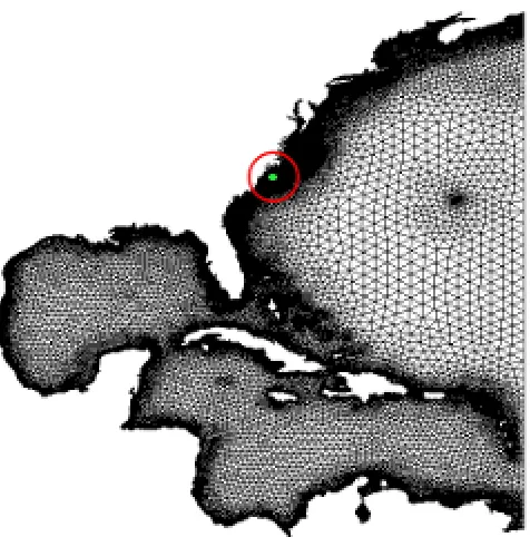
To appreciate the difference in scales between a typical ADCIRC domain and a coastal community, Fig. 1.1 shows the nodes of a mesh used by ADCIRC for hurricanes and tides on the east coast of the United States; this mesh ranges from Nova Scotia at its northern boundary to Venezuela at the southernmost. The dot within the ring in Fig. 1.1 appears small but represents a significant geographic region, from the perspective of coastal infrastructure assessment, which includes systems of roads and highways, bridges, barrier islands, beach dunes and other land features that are subject to inundation. The full-scale mesh depicted in Fig. 1.1 has over one million elements and requires approximately 600 CPU-hours on a modern processor to simulate a storm lasting four days in simulation time.
With runtime in mind the “local mesh” approach was developed and implemented in AD-CIRC. The local mesh approach consists of simulating each storm once and thereafter using the results obtained as boundary conditions for a significantly smaller mesh that is able to accurately simulate the storm in a reduced geographic area. A local mesh that is large enough to capture the impacts of different infrastructure design decisions in a moderately sized town is still small enough relative to the full-sized mesh to reduce the time required to simulate a storm by as much as 95% or more.
1.3
ADCIRC Background
ADCIRC is a coastal ocean hydrodynamic model with both three dimensional (3D) and two dimensional depth integrated (2DDI) versions (Luettich and Westerink 2004). For our purposes, the 2DDI version is used exclusively.
Figure 1.1: The scale of a full-sized ADCIRC mesh and a smaller local mesh (dot within the ring).
∂ζ ∂t +
1 Rcosφ
∂U H
∂λ +
∂(V Hcosφ) ∂φ
= 0, (1.1)
∂U ∂t +
1 RcosφU
∂U ∂λ + V R ∂U ∂φ − tanφ
R U +f
V =− 1 Rcosφ
∂ ∂λ
ps
ρ0
+g(ζ−αη)
+νT H ∂ ∂λ ∂U H ∂λ + ∂U H ∂φ
+ τsλ ρ0H
−τ∗U,
(1.2)
∂V ∂t +
1 RcosφU
∂V ∂λ + V R ∂V ∂φ + tanφ
R U+f
U =−1 R ∂ ∂φ ps ρ0
+g(ζ−αη)
+νT H ∂ ∂φ ∂V H ∂λ + ∂V H ∂φ
+ τsφ ρ0H
−τ∗V,
(1.3)
atmo-spheric pressure at the free surface; g = the acceleration due to gravity; η = the Newtonian equilibrium tide potential; α= the effective Earth elasticity factor; ρ0 = the reference density
of water;τsλ, τsφ= the applied free-surface stress; τ∗=Cf
√
U2+V2 H
= partial bottom friction term; Cf = the nonlinear bottom friction coefficient;νT = the depth-averaged horizontal eddy
viscosity coefficient.
To derive the GWCE formulation, a temporally-differentiated form of the depth averaged continuity equation is combined with a spatially-differentiated form of the depth averaged prim-itive momentum equations and multiplied by a constant,τ0, in time and space. The resulting
GWCE equation can be expressed as (Westerink et al. 1992)
∂2ζ
∂t2 +τ0
∂ζ ∂t + ∂ ∂x U∂ζ ∂t −U H
∂H ∂x −V H
∂U
∂y +f V H−H ∂ ∂x
p ρ0
+g(ζ−αη)
+ τsx ρ0
−(τ∗−τ0)U H
+ ∂
∂y
V∂ζ ∂t −U H
∂V
∂x −V H ∂V
∂y −f U H−H ∂ ∂y
p ρ0
+g(ζ−αη)
+ τsy ρ0
−(τ∗−τ0)V H
= 0. (1.4)
The GWCE and momentum equations are temporally discretized in a three-level scheme and a two-level scheme, respectively, leading to a decoupled solution to the two equations which allows for a sequential solution procedure (Westerink et al. 1992). The GWCE and momentum equations are then spatially discretized using a standard Galerkin finite element scheme, which operates on irregular linear triangles (Tanaka et al. 2010).
There are three primary routines that drive the physics of the model and that are executed in succession during every timestep. They are the GWCE routine, the wet/dry routine, and the momentum equation routine (Tanaka et al. 2010). The GWCE routine, which finds the elevation at each node in the domain for the current timestep by solving Eq. 1.4, has the ability to use either a spatially implicit or explicit method, employing an iterative Jacobi Conjugate Gradient method or a lumped mass matrix method, respectively. In this study, the implicit method is used. The wetting and drying routine determines the wet or dry status of each node in the domain via a series of checks based on elevation, velocity, wet/dry status in the previous timestep and wet/dry status of neighboring nodes (Luettich and Westerink 1999). The momentum routine finds the x and y velocity at each node in the domain for the current timestep by solving Eq. 1.2 and Eq. 1.3, respectively, explicitly using a lumped mass matrix. An extensive description of the mathematical formulation of ADCIRC is available from Luettich and Westerink (2004).
sub-Figure 1.2: The communication scheme between one of the subdomains and its four neighboring subdomains created from the mesh shown in Fig. 1.1.
domain being placed on a dedicated processor. At each timestep, information pertinent to the current state of the physics being modeled is communicated between neighboring subdo-mains using message passing. By using “ghost nodes,” each subdomain receives information at every node on its boundary via message passing from an adjacent subdomain (or from a boundary condition defined for the domain in cases where a subdomain shares a boundary with the complete domain), and only solves for nodes that are inside the domain; cf. Fig. 1.2. The physical information passed is the water surface elevation, depth averaged water velocity, flux per unit width and wet/dry status. The implicit version of the GWCE routine, when in use, also employs message passing for a global summation to find the residual norm of the solution.
1.4
Methodology
To implement a localized approach we consider the boundary data communicated in the parallel version of ADCIRC. This minimally invasive approach:
Table 1.1: Comparison of data used in parallel ADCIRC and in the local mesh approach.
Field Output File Communicated in
Parallel ADCIRC
Defined on Local Mesh Boundary
elevation fort.63 yes yes
x velocity fort.64 yes yes
y velocity fort.64 yes yes
wet/dry none yes no
• Takes advantage of the explicit nature of the momentum equation solver to assign velocity
values, effectively creating a new type of boundary condition in ADCIRC.
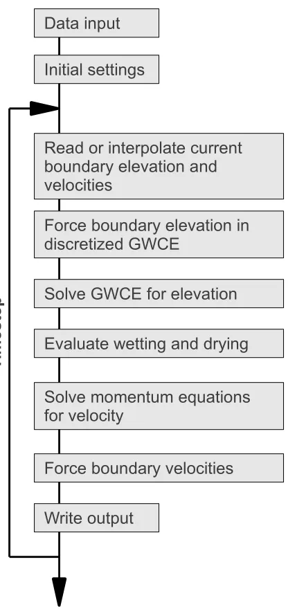
Because output data for hurricane simulations typically include elevation and vector velocity fields anyway, we make use of those results in the local mesh approach to enforce boundary conditions along the edges of the local mesh. Thus a full-scale, or “setup run,” is initially performed to generate those aperiodic boundary values. For nodes that are reported to be dry, the nodes’ topobathymetric heights above mean sea level (MSL) are used for their water surface elevations. An input file is created from the results obtained by the setup run that includes water surface elevation and the x and y velocities of each node on the boundary at a specified reporting interval, with intermittent values later determined by linear interpolation. A flowchart of the modified timestepping procedure is shown in Fig. 1.3.
Aspects of the parallel scheme that are not explicitly accounted for are the flux per unit width, nodal wet/dry status and the global summation. Because flux per unit width is simply the product of elevation and velocity, however, its value can be computed directly if elevation and velocity have been appropriately defined. Since wet/dry status is a binary value, inter-polation is not possible and the field would need to be reported and then forced in the local simulation at every timestep. While feasible, this has an undesirable impact on the procedure because of the size of the files required to report and then enforce the wet/dry status. Writing output at such a high frequency also adversely affects the runtime performance of ADCIRC. Be-cause the wet/dry routine is executed after the GWCE routine, we instead account for wet/dry status by forcing water surface elevation on the boundary and allowing the wet/dry routine to re-compute the status of boundary nodes, recognizing that there may be a small number of in-consistencies. Finally, because the global summation is used only in solving the global system it requires no representation in the local mesh approach. To summarize, a tabular representation of the physical fields used in the parallel implementation of ADCIRC and in the local mesh approach is shown in Table 1.1.
Data input
Initial settings
Solve GWCE for elevation
Evaluate wetting and drying
Solve momentum equations
for velocity
Write output
Read or interpolate current
boundary elevation and
velocities
Force boundary elevation in
discretized GWCE
Force boundary velocities
T
im
e
s
te
p
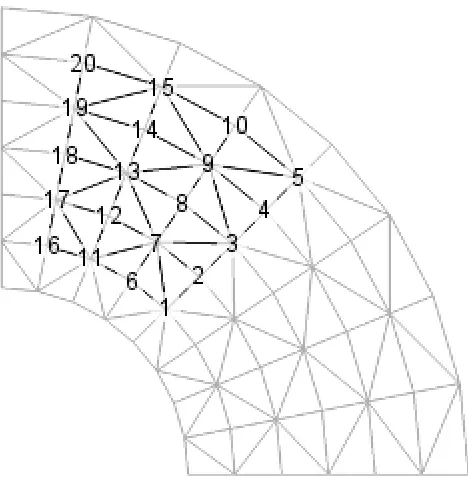
Figure 1.4: The mesh for the Quarter Annular example problem (gray), and an extracted local mesh (black) with node numbers corresponding to Table 1.2.
using PGI Fortran 11, GCC 4.5 and MPICH2 1.3.1. All simulations were executed on a single server rack containing 4 AMD Opteron 6168 (12 core) processors for a total of 48 cores with 64 gigabytes of RAM.
1.5
Quarter Annular Example
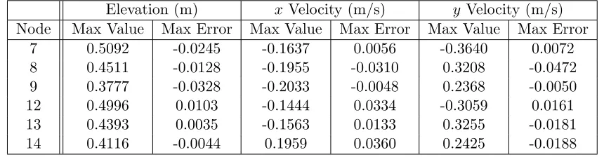
Table 1.2: Maximum values and errors seen at any timestep for elevation, x velocity and y velocity fields on the interior nodes of the local mesh for the QA example presented in Fig. 1.4.
Elevation (m) x Velocity (m/s) y Velocity (m/s)
Node Max Value Max Error Max Value Max Error Max Value Max Error
7 0.5092 -0.0245 -0.1637 0.0056 -0.3640 0.0072
8 0.4511 -0.0128 -0.1955 -0.0310 0.3208 -0.0472
9 0.3777 -0.0328 -0.2033 -0.0048 0.2368 -0.0050
12 0.4996 0.0103 -0.1444 0.0334 -0.3059 0.0161
13 0.4393 0.0035 -0.1563 0.0133 0.3255 -0.0181
14 0.4116 -0.0044 0.1959 0.0360 0.2425 -0.0188
1.6
Base Mesh for Storm Surge Modeling
For storm surge scenarios, a single mesh is used as the base topobathy and all local meshes are extracted from it. This base mesh contains about 520,000 nodes and 1,020,000 elements and encompasses the western North Atlantic Ocean, the Caribbean Sea and the Gulf of Mexico (Fig. 1.1 shows this domain). The nodes in this mesh have attributes of a surface directional effective roughness length, a value for Manning’snat the sea floor, a surface canopy coefficient and a primitive weighting in the continuity equation. The mesh has a steady open ocean boundary condition along its eastern edge; that is the water surface is specified as constant at MSL. External land boundaries along the North American coastline have no normal flow and free tangential slip. Islands inside the domain are represented by internal land boundaries.
1.7
Meteorological Forcing
Wind and pressure fields used to model hurricanes in the simulations presented below follow the Oceanweather Inc. (OWI) wind format, which describes pressure and velocity on a rectangular grid at regular time intervals. These data are interpolated in time to synchronize with the model time and interpolated in space to describe the meteorological state at the underlying mesh’s computational nodes. Garratt’s formulation is used to compute wind stress from wind velocity (Luettich and Westerink 2010; Garratt 1977):
Cd=
0.75 + 0.067s
103 ,
W = 0.001293Cdsv,
where Cd = wind drag coefficient; v = wind velocity 10 meters above the water’s surface;
1.8
Community Example
As an illustrative example, the local mesh approach is used to assess the inundation resulting from various levee breach scenarios for a hypothetical coastal community during a specified storm event. To do so, an initial storm surge simulation in ADCIRC is performed at full scale, which serves as the setup run for subsequent runs on a local mesh.
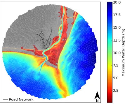
The community is a hypothetical example based on realistic topobathy and includes a small roadway network that is protected by an earthen levee while the coastline is protected by a barrier island. The community, however, is vulnerable to flooding from levee breaching or overtopping. The local mesh created (Local59) has 59,608 nodes, making its node count about 10% of the full mesh. The topobathy and associated road network of Local59 are shown in Fig. 1.5 and the maximum water depths of Local59 are shown in Fig. 1.6. This local mesh took approximately 50 CPU-hours to complete when run on 20 processors, compared to the 600 CPU-hours required to simulate the same storm on a full mesh.
Using Local59, six alternate topobathies are simulated for the storm event, each represent-ing a possible breach of the earthen levee protectrepresent-ing the city. Different breach locations yield different flooding scenarios, shown in Fig. 1.7. The results of these simulations may be used to populate network resilience models, which take into account the impact on the local infrastruc-ture and the probability of occurrence of each scenario (Piper 2009). For this example only one storm event is used, but the methodology is developed with the vision of a library of historical and synthetic storms being utilized (Niedoroda et al. 2008).
1.8.1 Model Settings
For this example scenario, the ADCIRC model is run for 3.9 days with a timestep of 0.5 s, receiving meteorological data every 1800 s. Time weighting factors for time steps k+ 1,k and k−1 are 0.35, 0.30 and 0.35, respectively. The wet/dry algorithm operates using a minimum water depth of 0.1 m and a minimum velocity for wetting of 0.05 m/s. A quadratic bottom friction law is specified, finite amplitude terms with wetting and drying of elements are enabled, and both the spatial and time derivative portions of the advective terms are included. All of the local mesh runs presented are forced on the boundary with data at every 1800 s unless otherwise noted.
1.8.2 Accuracy
The maximum surge levels in the local mesh are largely in agreement with those results, al-though there are some isolated areas of inconsistency on the barrier island, similar to the small inconsistencies introduced by the parallel version of ADCIRC.
In the examples that follow, we present two types of comparisons:
• (Local59 vs. FullSerial): The local mesh, Local59, compared with a full mesh run on
a single processor, and
• (Full15 vs. FullSerial): The full mesh run on 15 processors, Full15, compared with a
full mesh run on a single processor.
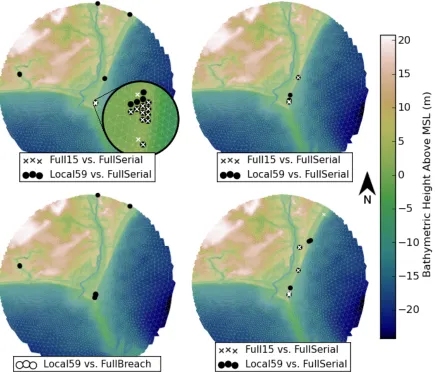
Water surface elevations in the local mesh are nearly identical to those in the full run on all but a very small number of nodes. The locations of errors larger than 15 cm in magnitude for Local59 and Full15 are shown in Fig. B.1(a). When comparing results, the water surface elevation for a node that is reported as dry is considered to be the node’s topobathymetric height above MSL. The Local59 mesh has five distinct clusters of inaccurate nodes, with 22 nodes being reported in total. Two of Local59’s clusters are along the coastline of the barrier island, one is in an interior shallow area and two are near narrow riverine bodies that flow through the boundary. Full15 results in only one cluster of nodes exceeding the tolerance of ±15 cm and contains 12 nodes in total. In Full15’s cluster, the nodes from the two samples
show considerable overlap, as seen in the inset of Fig. B.1(a).
The same method of comparing a local mesh to a full mesh run in parallel is used to evaluate the accuracy of the depth-averaged velocity values reported by the local mesh. Comparing the maximum velocity magnitude of each node in Local59 and Full15 to FullSerial, Fig. B.1(b) shows locations of nodes that have a discrepancy of more than 1.5 m/s. The locations of these nodes are qualitatively very similar to the locations of nodes that show a discrepancy in maximum water surface elevation.
To compare the velocities while accounting for both orientation and magnitude, we take the vector difference of the depth-averaged velocities at each time step and report the largest in magnitude. The locations of nodes whose velocities exceed a tolerance of ±1.5 m/s are shown in Fig. B.1(c). Both velocity metrics yield similar comparisons.
Figure 1.9: Runtime performance of differently sized meshes.
Moving to a scenario for which the localized approach was originally envisioned, we consider a modification to the interior of a local mesh that simulates the effect of a levee breach (the upper-left breach scenario shown in Fig. 1.7) To evaluate the quality of our results, we compare this case with a modification to the full mesh that contains the same breach (FullBreach). For this case, Local59 is still being forced on the boundary with data obtained from FullSerial, which does not contain the breach. Comparing the maximum elevations between the local and full runs shows 25 nodes with an error larger than 15 cm in magnitude (Fig. B.1(d)). None of these are located near the altered topobathy, indicating that the local mesh successfully captured the hydrodynamic effects of the levee breach.
To further validate the approach, multiple local meshes were created in and around the same coastal area, including meshes that are much smaller geographically and in node count. The results of these simulations are similar in quality to those above, cf. Appendix B. With respect to runtime, a linear relationship with the number of nodes in the local mesh is observed, as expected (Tanaka et al. 2010); cf. Fig. 1.9.
Figure 1.10: Flooding (outlined in white) on a local mesh created to demonstrate a mesh that is clearly too small for accurate results that nonetheless remains numerically stable.
mesh small enough to produce flooding across a boundary during a levee breach scenario (not present in the full run). Although the run completes successfully, the forced water surface elevations at the boundary are in conflict with the introduced flooding and numerous errors result. To create a local mesh is a simple and quick process, so little time is lost in the event that a larger mesh is deemed necessary.
1.9
Hurricane Isabel and Tides in the Cape Hatteras Region
of this example; it is purely an illustration of the performance of the local mesh approach when tides are considered along with the wind driven motions.
1.9.1 Model Settings
For the Cape Hatteras example the base run uses the same parameters as the previous example, with the exception that the model is run for 5.5 days with a 1.0 s timestep. Elevation and velocity data are reported every 1800 s, and are subsequently applied along the boundary of the local mesh. When tides are considered, a 20-day linear ramping period is used and the tidal spin-up phase lasts 45 days in total.
1.9.2 Accuracy
In applying the local mesh approach to the Cape Hatteras area it is observed that, ignoring tides, the local mesh performs very well for the wind field representing Isabel (2003), with only 3 nodes whose error exceeds 15 cm in magnitude when compared to a full run (Fig. 1.11(a)). The tidal run for the same local mesh also performs well when considering maximum water surface elevation, with only 4 having an error larger than 15 cm in magnitude (Fig. 1.11(b)). The tidal motions are captured well throughout the entirety of the run for both elevation and velocity fields, demonstrated by the time series at a randomly chosen node shown in Figs. 1.12 and 1.13 (node location shown in Fig. 1.11(c)). When wind and tides are included simultane-ously, however, the results are less accurate, yielding 32 nodes with errors exceeding 15 cm in magnitude (Fig. 1.11(d)), the subject of ongoing work.
1.10
Conclusions and Future Work
A key limiting factor in moving from the science of storm surge modeling to its practical appli-cation in engineering infrastructure assessment is one of scale: storm surge models necessarily operate over vast parts of the globe because that is the scale at which storms and hurricanes operate. We present an approach for storm surge modeling in ADCIRC that allows simulations to take place over a much smaller geographic region so that multiple changes in topography can be repeatedly considered and assessed in a fraction of the time required by a full simulation.
)assessed. Both small, benchmark problems and large-scale hurricane scenarios are presented, and examples are driven with tides, with wind fields, and with their combination, although improving accuracy in the latter case is a subject of ongoing work.
In terms of future work, we envision extending the methodology to include temporal as well as spatial localization, thereby improving efficiency and eliminating unnecessary computation time spent during the initial stages of a hurricane event and the tidal spin-up phase. Addi-tionally, the approach could be applied to the coupled version of ADCIRC and SWAN so that surface water waves could also be simulated and used to inform physical failure models of levees and other infrastructure components.
1.11
Acknowledgements
We would like to thank Dr. Rick Luettich and Dr. Brian Blanton for their help with the ADCIRC model and for providing the base grid, tide, and wind input files used herein. We would also like to thank Julie Maloney for her help plotting the results.
This material is based upon work supported by the U.S. Department of Homeland Secuirty under Award Number: 2008-ST-061-ND0001 and a Department of Homeland Security HS-STEM Career Development Grant.
1.12
Disclaimer
1.13
Notation
The following symbols are used in this paper:
α = the effective Earth elasticity factor;
Cd = wind drag coefficient;
Cf = the nonlinear bottom friction coefficient;
η = the Newtonian equilibrium tide potential;
f = 2Ω sinφ= the Coriolis parameter;
g = the acceleration due to gravity;
h = the bathymetric depth relative to the geoid;
H = ζ+h= the total water column;
λ, φ = degrees longitude and latitude;
νT = the depth-averaged horizontal eddy viscosity coefficient;
Ω = the angular speed of the Earth;
ps = the atmospheric pressure at the free surface;
R = the radius of the Earth;
ρ0 = the reference density of water;
s = kvk= wind speed 10 meters above the water’s surface;
t = time;
τ0 = the continuity equation multiplier;
τ∗ = Cf
√
U2+V2
H !
= partial bottom friction term;
τsλ, τsφ = the applied free-surface stress;
U, V = the depth-averaged horizontal velocities;
v = wind velocity 10 meters above the water’s surface;
W = wind stress;
Appendix A
Additions to the ADCIRC Code
A.1
ADCIRC Background
The ADCIRC model is primarily written in Fortran 90, the exception being the source code for METIS, a third party graph theory package that is used to decompose the domain during pre-processing for parallel runs. The source files that were altered by the local mesh implementation and a brief description of the responsibilities that are relevant to the local mesh are
• cstart.F
Set flags and coefficients used in time stepping for a simulation that is “cold started”
• global.F
Declaration of global variables and parameter constants
Set global parameter constants
Array declaration and memory allocation
• prep.F
Decompose boundary condition file(s) for subdomains
• timestep.F
Read boundary condition information
Solve GWCE
Wetting and drying
A.2
Changes in cstart.F
Added or altered code in lowercase.
!−−−−−−−−−−−−−−−−−−−−−−−−−−−−−−−−−−−−−−−−−−−−−−−−−−−−−−−−−−−−−−−−−−−−−−−−−−−−−
! THE PRIMARY 2D COLDSTART INITIALIZATION
!−−−−−−−−−−−−−−−−−−−−−−−−−−−−−−−−−−−−−−−−−−−−−−−−−−−−−−−−−−−−−−−−−−−−−−−−−−−−−
SUBROUTINECOLDSTART( )
. . .
open( 9 9 3 , f i l e=t r i m ( g l o b a l d i r ) / / ’ / ’ // ’ f o r t . 9 9 3 ’ )
read( 9 9 3 ,∗) l o c a l b o u n d
c l o s e( 9 9 3 ) . . .
! INITIALIZE THE ELEVATION SPECIFIED BOUNDARY CONDITION IF IT ! REQUIRES THE USE OF THE UNIT 19 FILE .
IF( (NOPE.GT . 0 ) .AND. ( NBFR.EQ. 0 ) ) THEN
IF(NSCREEN.NE . 0 .AND.MYPROC.EQ. 0 ) WRITE( S c r e e n U n i t , 1 1 1 2 )
WRITE( 1 6 , 1 1 1 2 )
IF(NSCREEN.NE . 0 .AND.MYPROC.EQ. 0 ) WRITE( S c r e e n U n i t , 1 9 7 7 )
WRITE( 1 6 , 1 9 7 7 )
1977 FORMAT( / , 1X, ’ELEVATION SPECIFIED INFORMATION READ FROM UNIT ’ , ’ 19 ’ , / )
OPEN( 1 9 ,FILE=TRIM(INPUTDIR) / / ’ / ’ // ’ f o r t . 1 9 ’ )
READ( 1 9 ,∗) ETIMINC
i f ( l o c a l b o u n d . eq . 1 ) then do j =1 , n e t a
read( 1 9 ,∗) e s b i n 1 ( j ) , r e a d 1 u ( j ) , r e a d 1 v ( j )
end do do j =1 , n e t a
read( 1 9 ,∗) e s b i n 2 ( J ) , r e a d 2 u ( j ) , r e a d 2 v ( j )
end do e l s e
DO J =1 ,NETA
READ( 1 9 ,∗) ESBIN1 ( J )
END DO DO J =1 ,NETA
READ( 1 9 ,∗) ESBIN2 ( J )
END DO e n d i f
ETIME1 = STATIM∗8 6 4 0 0 . D0 ETIME2 = ETIME1 + ETIMINC
ENDIF
. . .
A.3
Changes in global.F
Added or altered code in lowercase.
!−−−−−−−−−−−−−−−−−−−−−−−−−−−−−−−−−−−−−−−−−−−−−−−−−−−−−−−−−−−−−−−−−−−−−−−−−−−−−
! T h i s module d e c l a r e s a l l g l o b a l v a r i a b l e s t h a t a r e n o t e x c l u s i v e t o t h e 3D
! r o u t i n e s . The 3D e x c l u s i v e v a r i a b l e s a r e d e c l a r e d i n g l o b a l 3 D V S
!−−−−−−−−−−−−−−−−−−−−−−−−−−−−−−−−−−−−−−−−−−−−−−−−−−−−−−−−−−−−−−−−−−−−−−−−−−−−−
MODULEGLOBAL
. . .
integer : : l o c a l b o u n d , i l o c a l
r e a l( s z ) ,a l l o c a t a b l e : : r e a d 1 u ( : ) , r e a d 2 u ( : )
r e a l( s z ) ,a l l o c a t a b l e : : r e a d 1 v ( : ) , r e a d 2 v ( : )
r e a l( s z ) ,a l l o c a t a b l e : : uutemp ( : ) , vvtemp ( : ) . . .
!−−−−−−−−−−−−−−−−−−−−−−−−−−−−−−−−−−−−−−−−−−−−−−−−−−−−−−−−−−−−−−−−−−−−−−−−−−−−−
! A l l o c a t e s p a c e f o r A r r a y s d i m e n s i o n e d by MNOPE and MNETA
!−−−−−−−−−−−−−−−−−−−−−−−−−−−−−−−−−−−−−−−−−−−−−−−−−−−−−−−−−−−−−−−−−−−−−−−−−−−−−
SUBROUTINEALLOC MAIN2 ( )
IMPLICIT NONE
ALLOCATE ( ESBIN1 (MNETA) , ESBIN2 (MNETA) )
a l l o c a t e ( r e a d 1 u ( mneta ) , r e a d 2 u ( mneta ) )
a l l o c a t e ( r e a d 1 v ( mneta ) , r e a d 2 v ( mneta ) )
a l l o c a t e ( uutemp ( mneta ) , vvtemp ( mneta ) ) . . .
END SUBROUTINEALLOC MAIN2
. . .
A.4
Changes in prep.F
Added or altered code in lowercase.
!−−−−−−−−−−−−−−−−−−−−−−−−−−−−−−−−−−−−−−−−−−−−−−−−−−−−−−−−−−−−−−−−−−−−−−−−−−−−−
! ENTER, LOCATE, OPEN, AND READ THE ADCIRC UNIT 19
! GLOBAL APERIODIC ELEVATION BOUNDARY CONDITIONS FILE
!−−−−−−−−−−−−−−−−−−−−−−−−−−−−−−−−−−−−−−−−−−−−−−−−−−−−−−−−−−−−−−−−−−−−−−−−−−−−−
SUBROUTINEPREP19 ( ) . . .
double p r e c i s i o n e t i m i n c , e s b i n p , e s b i n p 2 , e s b i n p 3
double precision, a l l o c a t a b l e : : e s b i n ( : ) , e s b i n 2 ( : ) , e s b i n 3 ( : )
!OPEN FULL DOMAIN AND SUBDOMAIN FORT. 1 9 FILES
CALL OPENPREPFILES( 1 9 , ’APERIODIC ELEVATION BOUNDARY’ , 1 , NPROC, SDU, SUCCESS)
IF ( .NOT. SUCCESS) THEN
WRITE(∗,∗) ’WARNING: UNIT 19 FILES NOT PREPROCESSED. ’
RETURN ! NOTE EARLY RETURN
ENDIF
!ALLOCATE LOCAL ARRAYS
ALLOCATE ( ESBIN (MNETA) )
i f ( l o c a l b o u n d . eq . 1 ) then a l l o c a t e ( e s b i n 2 ( mneta ) )
a l l o c a t e ( e s b i n 3 ( mneta ) )
e n d i f
NBYTES = 8∗MNETA
CALLMEMORY ALLOC(NBYTES)
read( 1 9 ,∗) e t i m i n c
DOIPROC = 1 ,NPROC
write( sdu ( i p r o c ) ,∗) e t i m i n c
ENDDO
!WHILE ( NOT EOF ) READ NETA BC’ S FROM GLOBAL FILE
1000 CONTINUE
DO I =1 , NETA
i f ( l o c a l b o u n d . eq . 1 ) then
read( 1 9 ,∗,end=9999) e s b i n ( i ) , e s b i n 2 ( i ) , e s b i n 3 ( i )
e l s e
read( 1 9 ,∗,end=9999) e s b i n ( i )
ENDDO
DOIPROC= 1 ,NPROC
ESBINP = ESBIN (OBNODE LG( I , IPROC ) )
i f ( l o c a l b o u n d . eq . 1 ) then
e s b i n p 2 = e s b i n 2 ( o b n o d e l g ( i , i p r o c ) ) e s b i n p 3 = e s b i n 3 ( o b n o d e l g ( i , i p r o c ) )
e n d i f
i f ( l o c a l b o u n d . eq . 1 ) then
write( sdu ( i p r o c ) ,∗) e s b i n p , e s b i n p 2 , e s b i n p 3
e l s e
write( sdu ( i p r o c ) ,∗) e s b i n p
e n d i f ENDDO ENDDO
GO TO 1000
! CLOSE GLOBAL FILE AND ALL THE LOCAL FILES 9999 CLOSE ( 1 9 )
DOIPROC=1 , NPROC
CLOSE (SDU(IPROC ) )
ENDDO
d e a l l o c a t e( e s b i n )
i f ( l o c a l b o u n d . eq . 1 ) then d e a l l o c a t e( e s b i n 2 )
d e a l l o c a t e( e s b i n 3 )
e n d i f
NBYTES = 8∗MNETA
CALLMEMORY DEALLOC(NBYTES)
CALLMEMORY STATUS( )
RETURN
A.5
Changes in timestep.F
Added or altered code in lowercase.
SUBROUTINETIMESTEP( IT ) . . .
!COMPUTE THE WATER SURFACE ELEVATION FROM THE GWCE FORM OF THE 2D CONTINUITY EQ.
IF(CPRECOR) THEN
CALLGWCENEW( IT , TIME, TIMEH)
CALL MOM EQS NEW NC( ) #IFDEF CMPI
! IF RUNNING IN PARALLEL, UPDATE VELOCITIES AND FLUXES ON ALL PROCESSORS
CALLUPDATER(UU2, VV2,DUMY1, 2 )
CALLUPDATER(QX2, QY2,DUMY1, 2 ) #ENDIF
CALLGWCE NEW PC( IT , TIME, TIMEH)
ENDIF
IF(CGWCE ORIG) THEN
CALL GWCE ORIGINAL( IT , TIME, TIMEH)
ENDIF
IF(CGWCE NEW) THEN
CALLGWCENEW( IT , TIME, TIMEH)
ENDIF
! BEGIN WET/DRY SECTION . . .
!END WET/DRY SECTION
! 2DDI MOMENTUM EQUATION SOLUTION
IF ( C2DDI ) THEN
IF ( CME Orig ) THEN
CALL M o m E q s O r i gi n a l ( )
ENDIF
IF (CME New NC) THEN CALL Mom Eqs New NC ( )
ENDIF
IF ( ( CME New C1 ) .OR. ( CME New C2 ) ) THEN CALL Mom Eqs New Conserv ( )
ENDIF
IF (CPRECOR) THEN
CALL Mom Eqs Non Conserv pc ( )
ENDIF
#IFDEF CMPI
CALLUPDATER(UU2, VV2,DUMY1, 2 )
CALLUPDATER(QX2, QY2,DUMY1, 2 ) #ENDIF
ENDIF
END SUBROUTINE TIMESTEP
. . .
!−−−−−−−−−−−−−−−−−−−−−−−−−−−−−−−−−−−−−−−−−−−−−−−−−−−−−−−−−−−−−−−−−−−−−−−−−−−−−
! SUBROUTINE TO COMPUTE THE ELEVATION USING THE GWCE FORMULATION
! RE−WRITTEN TO CONFORM TO THE ADCIRC THEORY REPORT
! r . l . 06/22/2005
!−−−−−−−−−−−−−−−−−−−−−−−−−−−−−−−−−−−−−−−−−−−−−−−−−−−−−−−−−−−−−−−−−−−−−−−−−−−−−
SUBROUTINEGWCENEW( IT , TIME, TIMEH) . . .
! f o r a p e r i o d i c e l e v a t i o n and v e l o c i t y b o u n d a r y c o n d i t i o n
IF( (NBFR.EQ . 0 ) .AND. (NOPE.GT . 0 ) . and . ( l o c a l b o u n d . eq . 1 ) ) THEN IF(TIME .GT. ETIME2) THEN
ETIME1=ETIME2
ETIME2=ETIME1+ETIMINC
DO J =1 ,NETA
ESBIN1 ( J)=ESBIN2 ( J )
i f ( l o c a l b o u n d . eq . 1 ) then
r e a d 1 u ( j ) = r e a d 2 u ( j ) r e a d 1 v ( j ) = r e a d 2 v ( j )
READ( 1 9 ,∗) ESBIN2 ( J ) , r e a d 2 u ( j ) , r e a d 2 v ( j )
e l s e
READ( 1 9 ,∗) ESBIN2 ( J )
e n d i f END DO ENDIF
ETRATIO=(TIME−ETIME1) /ETIMINC
DO I =1 ,NETA NBDI=NBD( I )
ETA2(NBDI)=RAMPELEV∗( ESBIN1 ( I )+ETRATIO∗( ESBIN2 ( I )−ESBIN1 ( I ) ) )
i f ( l o c a l b o u n d . eq . 1 ) then
uutemp ( i ) = ( r e a d 1 u ( i ) + e t r a t i o∗( r e a d 2 u ( i ) − r e a d 1 u ( i ) ) ) vvtemp ( i ) = ( r e a d 1 v ( i ) + e t r a t i o∗( r e a d 2 v ( i ) − r e a d 1 v ( i ) ) )
e n d i f END DO ENDIF
. . .
END SUBROUTINEGWCENEW
. . .
! S u b r o u t i n e t o compute t h e v e l o c i t y and from t h a t t h e f l u x / u n i t w i d t h u s i n g
! a 2DDI non c o n s e r v a t i v e momentum e q u a t i o n .
!−−−−−−−−−−−−−−−−−−−−−−−−−−−−−−−−−−−−−−−−−−−−−−−−−−−−−−−−−−−−−−−−−−−−−−−−−−−−−
SUBROUTINEMOM EQS NEW NC( )
. . .
! a s s i g n x and y v e l o c i t y v a r i a b l e s t o t h e c o r r e c t v a l u e
i f( l o c a l b o u n d . eq . 1 ) then do i =1 , n e t a
uu2 ( nbd ( i ) ) = uutemp ( i ) vv2 ( nbd ( i ) ) = vvtemp ( i )
end do e n d i f
Appendix B
Additional Comparisons of Local
Appendix C
Summary of ADCIRC Files Used
The files necessary to run a local mesh simulation and their sources from the full-mesh files are presented in Table C.1.
The “Aperiodic Boundary Conditions” file is the only file mentioned that does not have a format already established by ADCIRC. In the implementation presented herein, it is of the format
A T I M E I N C for t =1 , NTS
for k =1 , N A B N
E ( t , k ) U ( t , k ) V ( t , k ) end k l o o p
end t l o o p
where ATIMEINC is the time increment for the file; NTS is the number of timesteps provided;
NABN is the number of aperiodic boundary nodes;E(t,k)is the elevation at time tat node k; U(t,k)is the x velocity at timetat nodek;V(t,k)is the y velocity at timetat nodek. This is the same format as the existing “Non-Periodic Elevation Boundary Condition” (fort.19) and “Non-Periodic Normal Flux Boundary Condition” (fort.20) files, but contains three values per line instead of one.
Table C.1: Source information for files necessary to complete a local mesh simulation.
File Description Source File(s)
(From Full Mesh) Notes