Bayesian ROC curve estimation under binormality using a partial likelihood based on ranks

Bayesian ROC curve estimation under binormality using a partial

likelihood based on ranks

By

Jiezhun Gu

Subhashis Ghosal

Department of Statistics, North Carolina State University, Raleigh, North Carolina

27695-8203, U.S.A.

[email protected]

[email protected]

Institute of Statistics Mimeo Series # 2598

Summary

There are various methods to estimate the parameters in the binormal model for the

ROC curve. In this paper, we propose a conceptually simple and computationally accessible

Bayesian estimation method using a partial likelihood based on ranks. Posterior consistency

is also established. We compare the new method with other estimation methods and

con-clude that our estimator generally performs better than its competitors.

Some key words: Binormal model; MCMC; Rank-based partial likelihood; ROC curve; Posterior consistency.

1. Introduction

First introduced in the context of medical diagnostic test by Lusted (1960), Receiver Operating

Characteristic (ROC) analysis has become a unique tool in measuring the accuracy of diagnostic

tests due to its ability to show two alternatives (true positive and false positive) simultaneously

(Swets, 1973). In the general diagnostic setting, with the gold standard for the truth, each patient is

known from either non-diseased or diseased population. Diagnostic result is obtained by comparing

the diagnostic test value with the subjective decision threshold value. For example, Let X and

Y denote two diagnostic test variables from non-diseased and diseased populations, respectively. Based on a decision threshold value ct ∈ R, a patient from X (or Y) is diagnosed as positive if

scales of false positive fraction and true positive fraction. The ROC curve is increasing, invariant

under any monotone increasing transformation on diagnostic variablesX andY and the area under the curve can be interpreted as Pr(Y > X) (Bamber, 1975). This may be used to quantify the accuracy of different diagnostic tests if the curves do not cross. These inherited features has made

ROC analysis flourishing; see the reviews by Swets & Pickett (1982), Hanley (1989), Zhou et al.

(2002) and Pepe (2003).

Throughout the literature of the estimation methods of ROC curves for continuous diagnostic

variables based on independent observations, the most popular assumption is the binormality, which

assumes that the diagnostic test variables of the non-diseased and diseased groups are normally

distributed after some monotone increasing transformationH. That is (without loss of generality),

H(X) ∼ Normal(0,1) and H(Y) ∼ Normal(µ, σ2_{), with the convention that µ > 0. Then the}

binormal ROC curve is given by R(t) = Φ(a+bΦ−1_{(t)), where a = µ/σ and b = 1/σ. The}

corresponding AUC has a closed expression Φ(a/√1 +b2_{) (McClish, 1989).}

The existing estimation methods for continuous diagnostic variables based on independent

ob-servations under binormality assumption is abundant. Metz et al. (1998) treat the continuous

diagnostic test data as an extension of ordinal data by grouping the rank-ordered data into some

fixed I categories conditional on the truth state runs. Hence, both binormal parameters and the nuisance parameters of I−1 category boundary points can be estimated by maximum likelihood method (Dorfman & Alf, 1969) at the same time. Zou & Hall (2000) directly construct a

rank-based likelihoodL(µ, σ2_{|ranks of Y}

1, . . . , Yn among the data) and obtain maximum likelihood (ML)

estimates ofµ, σ2 _{approximated by using a Monte Carlo procedure. Based on the observation that}

R(t) = Pr( ¯F(Y)≤t) = E(1( ¯F(Y)≤t)), Pepe (2000) and Alonzo & Pepe (2002) present a general-ized linear model using probit link. Cai & Moskowitz (2004) propose a maximum profile likelihood

and pseudo-maximum likelihood method which are more efficient than Metz et al. (1998)’s LABROC

and Alonzo & Pepe (2002)’s GLM when the sample size is large. These estimators are invariant

under monotone increasing transformations on the diagnostic variables. The estimators based on

the methods of modeling distribution function do not satisfy the invariant property in general, such

as a generalized least squared procedure (Hsieh & Turnbull, 1996), Box-Cox transformation method

(Zou & Hall, 2000); see reviews by Zhou et al. (2002), Pepe (2003), Cai & Moskowitz (2004) for

more details.

Here, we will propose a Bayesian curve estimation method under binormality using a partial

treat the transformation as latent and to construct a Bayes estimator given the maximal invariant,

namely, the ranks. A similar situation arises in Gaussian copula model (Hoff, 2006). We also show

the posterior consistency conditional on the ranks of the samples except possibly for a collection

of true parameter values of Lebesgue measure zero by applying Doob’s Theorem (cf. Ghosh &

Ramamoorthi, 2003).

The paper is arranged as follows. Our method is proposed in Section 2. Posterior consistency

is studied in Section 3. Simulation studies and real data analysis are shown in Section 4 and 5,

respectively.

2. BAYESIAN RANK-BASED PARTIAL LIKELIHOOD ESTIMATION

METHOD

2

_·

1. Notation of truncated normal distribution

Two-sided-truncated normal with non-truncated normal mean µ, variance σ2 _{and corresponding}

truncation region (e1, e2) is denoted as TN(µ, σ2,(e1, e2)); its density can be expressed asfT N(x) =

φ(x)/Re2

e1 φ(x)dx, whene1 < x < e2; fT N(x) = 0, otherwise. Hereafterφand Φ denote the

proba-bility density function (pdf) and cumulative density function (CDF) of the standard normal

distri-bution, respectively; Φµ,σ denotes the CDF of the normal distribution with mean µ and standard

deviationσ, that is Φµ,σ(x) = Φ((x−µ)/σ).

2

_·

2.

A partial likelihood and the corresponding Bayesian procedure

A Binormal model assumes thatX1, . . . , Xm∼independently and identically distributed (i.i.d.) F,

Y1, . . . , Yn ∼i.i.d. G, X and Y are continuous and independent, without loss of generality, there

exists monotone increasing transformationH, such that

Zi=H(Xi)∼i.i.d. Normal(0,1), Wj =H(Yj)∼i.i.d. Normal(µ, σ2), (2·1)

S=SN = (X,Y),X= (X1, . . . , Xm), similar notations forY,Z,W,

combined ranksRN =R(SN) = (R1N, . . . , RN N), N=m+n,

labelsL=L(S) = (L1N, . . . , LN N), whereLiN = 0 (respectively, 1) ifSi from X(respectively,Y).

we can define a setDobs invariant underH as follows:

Dobs ={(z,w)∈Rm+n:R(z,w) =R(S), L(z,w) =L(S)},

={(z,w)∈Rm+n:Zk < zk < Zk, Wl< wl< Wl, L(z, w) =L(S)}, (2·2)

where z = (z1, . . . , zm),w = (w1, . . . , wn), Zk = maxi{Zi : Xi < Xk} ∨maxj{Zj : Yj < Xk}, Zk = mini{Zi :Xk < Xi} ∧minj{Zj :Xk < Yj},Wl= maxi{Wi :Xi< Yl} ∨maxj{Wj:Yj< Yl}, Wl = mini{Wi : Yl < Xi} ∧minj{Wi : Yl < Yj}, for all k = 1, . . . , m, l = 1, . . . , n. Hence, a

rank-based partial likelihood can be defined based on this invariant set (2·2) as

Pr((z,w)∈Rm+n :R(z,w) =R(S), L(z,w) =L(S)|µ, σ)

= Pr((z,w)∈ Dobs|µ, σ, R(z,w) =R(S), L(z,w) =L(S)). (2·3)

However, evaluation of (2·3) involves high dimensional integrations, and hence direct

computa-tion of the maximum partial likelihood estimates will be computacomputa-tionally extremely challenging. An

alternative is to adopt the Bayesian approach. The Bayes partial likelihood estimator (BPL) may

be defined as the posterior mean of (µ, σ), where the posterior distribution is given by

π(µ, σ|R(S), L(S)). (2·4)

We shall use a data augmentation technique and implement Gibbs sampling to compute the

posterior in (2·4). More specifically, letting (Z,W) be the augmented variables, we shall de-scribe a procedure to sample from the conditional distribution of ((µ, σ)|Z,W, R(S), L(S)) and ((Z,W)|µ, σ, R(S), L(S)); see Section 4 for details.

3. CONSISTENCY OF THE POSTERIOR

Let (µ0, σ0) be the true value of (µ, σ). It is important to know if the consistency of the

poste-rior at (µ0, σ0) holds, i.e., whether the posterior distribution concentrates around (µ0, σ0) (Ghosh

& Ramamoorthi, 2003). Assume that the disease prevalence is asymptotically stable, i.e. when

Theorem 1. Suppose thatS_∼(1−λ)F+λG, and assume that binormality (2·1) holds conditional on the labels,(µ, σ)has joint prior densityπ(µ, σ)>0a.e. overR×R+with respect to the Lebesgue measureν. Then for(µ0, σ0)a.e. [ν], and for any neighborhoodU0 of(µ0, σ0), we have that

lim

N→∞

π((µ, σ)∈ U0|R(S), L(S)) = 1 a.s. [P

∞

µ0,σ0,H], (3·1)

whereP∞

µ0,σ0,H denotes the joint distribution of allX’s andY’s under the binormal model (2·1) with

(µ0, σ0) as the true value of(µ, σ).

Proof. BecauseSi∼i.i.d. (1−λ)F+λG, thenUi= ((1−λ)F+λG)(Si) are i.i.d. Uniform(0,1). Hence, we have

Uk = lim

N→∞ RkN

N+ 1 for all fixed k, (3·2)

whereRkN is the rank of thekth _{element among the totalN observations. This result is contained}

in the proof of Theoremaon page 157 of H´ajek & ˇSid´ak (1967).

Notice unconditionally,Ui= ((1−λ)Φ +λΦµ,σ)(Ni) are i.i.d. Uniform(0,1), whereNi=H(Si).

Based on the sample size N, we denote a subsequence labeling the observations conditionally from

F as (i1, . . . , im). Hence, conditionally onLijN = 0, j = 1, . . . , m, Nij ∼Normal(0,1) and Uij = ((1−λ)Φ +λΦµ,σ)(Nij)∼i.i.d. gµ,σ(say), which belongs to a regular parametric family indexed by parameters (µ, σ). More specifically, Cram´er type regularity conditions can be verified by applying the inverse function theorem. Thus some consistent estimator for (µ, σ) can be easily obtained, such as the MLE, a Bayes estimator or the method of moment estimator. Hence, there exist a series of

functionshN andh, such that (µ, σ) = lim

N→∞

hN(Ui1, . . . , Uim) =h(Ui1, Ui2, . . .), say.

Therefore, there exist functions ˜h,f1, f2, . . ., conditional on observations fromF,

(µ, σ) =h(Ui1, Ui2. . .)

=h( lim

N→∞

f1(RN), lim N→∞

f2(RN), . . .)

= ˜h(R(SN) : N ≥1) a.s. [P∞ µ0,σ0,H],

where RN = R(SN) is defined in (2·1). By Doob’s Theorem (cf. Ghosh & Ramamoorthi, 2003,

page 22 Theorem 1.3.2.), the consistency of posterior (3·1) at (µ0, σ0) holds a.e. [π], and hence at

(µ0, σ0) a.e. [ν].

of an analog of the Lebesgue measure implies that the exceptional set of points where the posterior

may be inconsistent is null when measured with respect to the prior only. This severely dilutes the

importance of the conclusion since what is null with respect to a given prior may be quite large when

measured with respect to another prior. In the present case, existence of a dominating Lebesgue

measure removes this arbitrariness.

4. SIMULATION STUDIES

We compare the BPL estimator of binormal model for ROC curve obtained by (2·4) with other

methods, such as maximum profile likelihood estimator (MLE) and pseudo maximum likelihood

estimator (PMLE) proposed by Cai & Moskowitz (2004), binary regression approach (GLM) by

Alonzo & Pepe (2002), and LABROC by Metz et al. (1998) through the same data generating

scheme in Cai & Moskowitz (2004). We choose the commonly used improper priorπ(µ, σ2)∝1/σ2

and define the same initial values of µ = 3, σ = 2 for each simulated data set. Gibbs sampling procedure from the posterior (2·4) is described as follows using the same denotation in (2·1):

1. Generate (X1, . . . , Xm) ∼ i.i.d. Normal(0,1), (Y1, . . . , Yn) ∼ i.i.d. Normal(µ, σ2), order

the combined vector (X,Y) denoted as OS(X,Y) and record the corresponding labels as

L(OS(X,Y));

2. Generate the initial values (Z,W) satisfying L(OS(Z,W)) =L(OS(X,Y));

3. Start the iterations:

(1) Conditional onµ, σ, updateQ=OS(Z,W) = (Q[1], . . . , Q[N]) with constraint ((Z,W)∈ Dobs|µ, σ), equivalently, satisfying L(Q) = L(OS(X,Y)) through the following sequential

truncated normal componentwise simulations (i= 1, . . . , N):

Q(new)[i]∼

 



TN(0,1,(Q[i−1], Q[i+ 1])), whenLiN = 0; TN(µ, σ2_{,(Q[i−1], Q[i+ 1])), whenLiN = 1,}

whereQ[0] =−∞,Q[N+ 1] =∞.

(2) Update Z (or W) values based on Q(new) _{and L(OS(X,Y)), i.e., every component of}

vectorZbelongs to the set

similarly, every component of vectorWbelongs to the set

{Q(new)_{[i] :LiN = 1, i= 1, . . . , N},}

(3) Updateµandσby their posterior distributions as

σ2|rest∼ inverse gamma ((n−1)/2,(n−1)s2w/2),

µ|rest∼Normal( ¯Wn, σ2/n),

wheres2

w= Pn

j=1(Wj−Wn¯ )2/(n−1), ¯Wn =

Pn

j=1Wj/n.

4. After burn-in, by averaging out the Gibbs samples, we can calculate ˆµ,ˆσ2_{, and record ˆa=}

ˆ

µ/σ,ˆ ˆb= 1/σˆfor the given dataX,Y. In the mean time, we can calculate 100(1−α)% credible intervals for ˆa and ˆb as (qa,α/2, qa,1−α/2) and (qb,α/2, qb,1−α/2), where qa,α/2 and qa,1−α/2)

denote α/2 and 1−α/2 quantiles of Gibbs samples of a, respectively; similar definition of

qb,α/2,qb,1−α/2forb.

We calculate the bias and the MSE of the estimates using methods BPL, MLE, PMLE, GLM

and LABROC. The true values of parameters are defined asa= 1.245 andb= 0.667, equivalently,

µ = 1.868, σ = 1.5. Simulation results in Table 1 also includes the information contained in Cai & Moskowitz (2004). For limited simulation results not shown in Table 1, when the sample size

exceeds one thousand, mean square errors obtained by BPL tend to be much smaller than those by

MLE, PMLE, GLM and LABROC methods.

Table 1: Estimates of binormal ROC’s parameter

a

and

b

using methods BPL, MLE, PMLE,

GLM and LABROC where we abbreviate it as LAB inside the table. Our BPL estimate is

based on 100 simulated data sets, 95000 Gibbs samples with 100000 iterations and burn-in

at 5000. The other estimates are based on 1000 simulated data sets.

m Bias Mean square error

n BPL MLE PMLE GLM LAB BPL MLE PMLE GLM LAB 50 a .071 .079 .064 .034 .032 .051 .063 .064 .059 .059 50 b -.004 .043 .062 -.009 .002 .020 .022 .022 .022 .022 200 a -.007 .026 .018 .013 .002 .010 .125 .138 .126 .128 200 b -.006 .014 .017 -.004 .001 .004 .048 .051 .052 .049

In order to check whether the frequentist variability of the estimate can be asymptotically

average of the estimated standard error estimator and MCMC standard error obtained by PMLE

and BPL respectively denoted as Ave( ˆSE) in Table 2, coverage probabilities of the 95% confidence interval for the estimatesaandb. Simulation results in Table 2 also contains the information in Cai & Moskowitz (2004).

Table 2: Sampling properties of BPL and PMLE. Our BPL estimate is based on 100

simulated data sets, 95000 Gibbs samples with 100000 iterations and burn-in at 5000. The

PMLE estimate is based on 1000 simulated data sets.

m Sampling SE Ave( ˆSE) Coverage n BPL PMLE BPL PMLE BPL PMLE 50 a .215 .245 .234 .248 .98 .974 50 b .141 .135 .143 .193 .97 .968 200 a .098 .116 .112 .113 .96 .945 200 b .066 .070 .064 .073 .95 .949

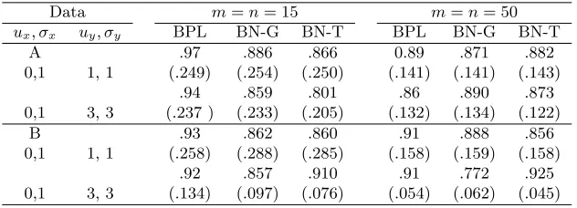
Besides considering the performance of the estimators in the binormal model, we also compare

the accuracy of the estimators of ROC functional AUC obtained by our BPL with BN-G (ROC

GLM method by Pepe, 2000), BN-T Box-Cox (Zou & Hall, 2000). Coverage probabilities of AUC

and corresponding average lengths of the 90% CI (shown beneath in the parathesis ) are displayed

in Table 3.

Based on the limited simulation results shown above, we conclude that BPL estimator of (a, b) has considerably smaller MSE than the estimators given by MLE, PML, GLM, LABROC methods

in this simulation setting. When the sample size increases, although BPL estimator tends to have

slightly larger bias, its mean square error is much smaller than the others in Table 1. Compared

to PMLE, our BPL estimates have smaller sampling variation in most cases and similar coverage

probabilities in Table 2. Also, because the simulation results of Ave( ˆSE) which shows the sampling variability and asymptotic variability using BPL and PMLE method, respectively, are not far from

those of Sampling SE which reflects the frequentist variability using BPL and PMLE methods, we can

use the sampling variability to estimate the frequentist variability. Moreover, compared to PMLE,

our BPL estimator performs better when estimatingbbased on sample sizem=n= 50. Compared to BN-G and BN-T, our BPL estimator tends to have larger average length of CI for AUC but with

much higher coverage probability when the simulated data sets are from location-scale exponential

distributions. When the data are from lognormal which means the binormality assumption holds

Table 3: Coverage probabilities of AUC and corresponding average lengths of the 90% CI

shown beneath in the parathesis obtained by BPL, BN-G and BN-T methods. Our BPL

estimate is based on 100 simulated data sets and corresponding 100000 iterations burn-in

at 5000, BN-G and BN-T’s estimates are based on 1000 simulated data sets and

corre-sponding 1000 resamples. Simulated data sets are generated by lognormal, location-scale

exponential distributions (abbreviated as

A, B

, respectively) with different combinations of

the parameters (A:

X

and

Y

datesets are generated from the lognormal with corresponding

normal parameters (

u

, σ

) and (

u

, σ

), respectively; B:

X

and

Y

are generated from the

exponential distribution with rate=0.5 and the location and scale parameters (

u

, σ

) and

(

u

, σ

), respectively). The grid points on [0,1] is chosen with equal interval length 0.05.

Data m=n= 15 m=n= 50 ux, σx uy, σy BPL BN-G BN-T BPL BN-G BN-T

A .97 .886 .866 0.89 .871 .882 0,1 1, 1 (.249) (.254) (.250) (.141) (.141) (.143)

.94 .859 .801 .86 .890 .873 0,1 3, 3 (.237 ) (.233) (.205) (.132) (.134) (.122)

B .93 .862 .860 .91 .888 .856 0,1 1, 1 (.258) (.288) (.285) (.158) (.159) (.158)

.92 .857 .910 .91 .772 .925 0,1 3, 3 (.134) (.097) (.076) (.054) (.062) (.045)

5. REAL DATA ANALYSIS

We will use the data set published by Wieand et al. (1989). This study was based on 51 patients

as control group diagnosed as pancreatitis and 90 patients as cases group diagnosed as pancreatic

cancer by two biomarkers, which were a cancer antigen (CA 125) and a carbohydrate antigen (CA

19-9). The purpose was to decide which marker would better distinguish case group from control

group. We will compare our BPL estimator with MLE and PMLE by Cai & Moskowitz (2004), Zou

& Hall (2000), GLM (Alonzo & Pepe, 2002) and LABROC (Metz, et al. 1998) using biomarker CA

125 for illustration. Our BPL estimate is based on 95000 Gibbs samples with 100000 iterations and

burn-in at 5000. We use the same priors as described in Section 4. Both of the initial values ofaand

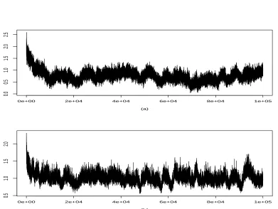
b are chosen to be equal to 2. Simulation results in Table 4 also reflect the information contained in Cai & Moskowitz (2004). Convergence of MCMC is examined by trace plot of MCMC samples

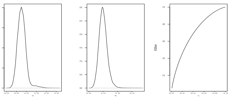
in Figure 1. The density plots of MCMC samples ofa, b and our BPL estimate of ROC curve are shown in Figure 2, respectively. Compared to the other estimates, our BPL estimate tends to have

Table 4: Real data analysis CA-125: comparison of estimates (standard errors) of binormal

parameters obtained by our BPL and other semiparametric methods.

BPL MLE PMLE Zou & Hall GLM (2002) LABROC a .748(.188) .76(.191) .719(.198) .727(.190) .778(.197) .720(.185) b 1.024(.139) 1.065(.140) 1.020(.148) 1.007(.142) 1.017(.167) 1.002(.137)

0e+00 2e+04 4e+04 6e+04 8e+04 1e+05

0.0

0.5

1.0

1.5

2.0

2.5

(a)

0e+00 2e+04 4e+04 6e+04 8e+04 1e+05

0.5

1.0

1.5

2.0

(b)

0.0 0.5 1.0 1.5 2.0 2.5

0.0

0.5

1.0

1.5

2.0

a

0.5 1.0 1.5 2.0

0.0

0.5

1.0

1.5

2.0

2.5

3.0

b

0.0 0.2 0.4 0.6 0.8 1.0

0.2

0.4

0.6

0.8

1.0

c

ROCBNcurve

Figure 2: Density plot of intercept (a) and slope (b) and ROC estimate (c) by BPL method

ACKNOWLEDGEMENTS

Research of the authors is partially supported by NSF grant number DMS-0349111.

APPENDIX

Matlab codes for BPL method

% Given information x m observations from nondiseased group

% y, n observations from disease group

% grid, the length of even interval of false positive fraction

% NSCAN, an integer of MCMC iterations

% burnin, an integer of burn-in

% gap, an integer of lag

% a0=a(1), initial value ofµ

% b0=b(1), initial value ofσ

% Help function–generate size=nsample random variables from truncated normal with

non-truncated normal meanµ, varianceσ2 _{and corresponding truncation region (e} 1, e2)

function [TN2] =TN2(nsample,µ,σ,e1,e2)

xq=ones(nsample,1);

din= normcdf(e2,µ,σ)- normcdf(e1,µ,σ);

u=rand(1,1);

xq(i)=norminv(din*u+normcdf(e1,µ,σ),µ,σ);

end;

TN2=xq;

% start the main codes

z=[x;y];%(m+n)*1 matrix

idd=[zeros(m,1);ones(n,1)];

[temp, index]=sortrows(z);

id=idd(index); %configuration of combined ordered statistics denoted as id

orid=1:(m+n);

% start to get the iniatial values R=order(Z,W)

Rtemp=zeros(m+n,1);

Rtemp(id==1)=sort(normrnd(a0,b0,n,1));%fill in W initial values

indexy=orid(id==1);%get the corresponding indices of W’s initial denoted as indexy

if (indexy(1)>1) %fill in Z initial values

Rtemp(1:(indexy(1)-1))=sort(TN2((indexy(1)-1),0,1,-100,Rtemp(indexy(1))));

end;

gum=ones(size(indexy,2),2);

gum(:,2)= [diff(indexy) -1]-1;

gum(:,1)=indexy;

for i=1:n

if (gum(i,2)>0)

Rtemp((gum(i,1)+1):(gum(i+1,1)-1))=sort(TN2(gum(i,2),0,1, Rtemp(gum(i,1)), Rtemp(gum(i+1,1))));

end;

end;

R=Rtemp;

% start Gibbs sampling

for j=1:NSCAN

% update R based on current values a(j) and b(j)

if (id(i)==0)

R(i)=TN2(1,0,1,-100,R(2));

else

R(i)=TN2(1,a(j),b(j),-100,R(2));

end;

for i=2:(m+n-1)

if (id(i)==0)

R(i)=TN2(1,0,1,R(i-1),R(i+1));

else

R(i)=TN2(1,a(j),b(j),R(i-1),R(i+1));

end;

end;

i=(m+n);

if (id(i)==0)

R(i)=TN2(1,0,1,R(m+n-1),100);

else

R(i)=TN2(1,a(j),b(j),R(m+n-1),100);

end;

% update Z, W values based on R

Z=R(id==0);

W=R(id==1);

vrate=var(W)*(n-1)/2;

% update a and b by (Z,W)

b(j+1)=sqrt(1/gamrnd((n-1)/2, 1/vrate));

a(j+1)=normrnd(mean(W), b(j+1)/sqrt(n),1,1);

end;

% end of Gibbs sampling

% BPL estimate of intercept and slope in the binormal model for ROC

BPLintercept=mean(a(gib)./b(gib));

BPLslope=mean(1./b(gib));

R

_EFERENCES

Alonzo, T. A. and Pepe, M. S. (2002). Distribution-free ROC analysis using binary regression

techniques. Biostatistics 3, 421-432.

Bamber, D. (1975). The area above the ordinal dominance graph and the area below the receiver

operating graph. Journal of Mathematical Psychology 12, 387–415.

Cai, T. & Moskowitz C. (2004). Semiparametric estimation of the binormal ROC curve. Biostatis-tics 5(4), 573–586.

Dorfman D. D. & Alf, E. (1969). Maximum likelihood estimation of parameters of signal-detection

theory and determination of confidence intervals–rating method data. Journal of Mathemat-ical Psychology 6, 487–496.

Ghosh, J. K. & Ramamoorthi, R. V. (2003). Bayesian Nonparametrics. Springer-Verlag, New York.

Hanley, J. A. (1989). Receiver operating characteristic (ROC) methodology: the state of the art.

Critical Reviews Diagnostics Imaging 29, 307–335.

Hoff, P. D. (2006). Extending the rank likelihood for semiparametric copula estimation. (http :

//arxiv.org/abs/math/0610413).

H´ajek, J. & ˇSid´ak, Z. (1967). Theory of Rank Tests. Academic press, New York.

Hsieh, F. S. & Turnbull, B. W. (1996). Nonparametric and semiparametric estimation of the

receiver operating characteristic curve. The Annals of Statistics 24, 25-40.

Lusted, L. B. (1960). Logical analysis in roentgen diagnosis. Radiology 74, 178-193.

Metz, C. E., Herman, B. A. & Shen, J. (1998). Maximum likelihood estimation of receiver operating

characteristic (ROC) curves from continuously-distributed data. Statistics in Medicine 17, 1033–1053.

McClish, D. K. (1989). Analyzing a portion of the ROC curve. Medical Decision Making 9, 190–195.

Pepe, M. S. (2000). An interpretation for the ROC curve and inference using GLM procedures.

Pepe, M. S. (2003). The Statistical Evaluation of Medical Tests for Classification and Prediction.

Oxford Statistical Science Series, Oxford University Press.

Swets, J. A. (1973). The relative operating characteristic in psychology. Science 182, 990–1000.

Swets, J. A. & Pickett, R. M. (1982). Evaluation of Diagnostic Systems: Methods from Signal Detection Theory. Academic Press, New York.

Zhou, X. H., McClish, D. K. & Obuchowski, N. A. (2002). Statistical Methods in Diagnostic Medicine. John Wiley & Sons, Inc., New York.

Zou, K. H. & Hall, W. J. (2000). Two transformation models for estimating an ROC curve derived