Approximate analysis of a multi-class open queueing network with class blocking and push-out

Approximate Analysis of a .

.

Multi-Class Open Queueing Network

with Class Blocking and Push-Out

r

,TUlin

Atmaca

~~~}!

.HarryG. Perros

Yves

Dallery

Center for Communications

and

Signal Processing

Department Electrical

and

Computer Ellgineering

North Carolina State University.

TR-91/2

Approximate Analysis of a

Multi-Class Open Queueing Network with

Class Blocking and Push-out'

by

Tiilin Atmaca Laboratoire MASI, Universite Pierre et Marie Curie

4Place Jussieu

75252 Paris Cedex 05,France

Harry G.

Perros-Computer Science Department, and Center for Communication and Signal Processing

North Carolina State University

Raleigh, NC 27695-8206, USA

Yves Dallery Laboratoire MASI, Universite Pierre et Marie Curie

4 PlaceJussieu

75252 ParisCedex 05, France

January1991

ISupported in part byNATO under grant noeRG900580.

Abstract:

We study a multi-class queueing network which consists of a finite capacity node (node 0) linked

to M parallel finite capacity nodes (nodes 1 to M). M classes of customers are assumed. All

customers first join node

O.

A class i customer after completion of its service at node

°

always joins the ith node. All service times and inter-arrival times are assumed to be exponentially

distributed. The service priority at node 0 is head-of-line with pre-emption. When node i

(i= 1,2,...,M) is full, node0cannot process class i customers. In addition to the service priorirty at

node 0, push-out is employed. That is, a customer that arrives at node 0 when the node is full,

takes the space of a customer which has the lowest priority among the customers already in the

node. If all customers in the node have a higher or equal priority, then the arriving customer is

lost. This queueing network is analyzed approximately by decomposing it into individual nodes,

and then analyzing each node separately. Node0 is analyzed using a class by class decomposition.

The approximation algorithm has been validated using simulation, and the approximate results

have a good error.

1. Introduction

Queueing networks with blocking have recently received a lot of attention (see

r

I]. and (8

I).

Blocking arises as a consequence of the finiteness of the buffers. In many real systems, and

especially in computer networks and in manufacturing systems, the finiteness of buffers has a

significant effect on the performance. Thus, it is important to be able to analyze queueing network models with fmite capacity queues.

So far, most of the work on queueing networks with blocking has been devoted to single-class

queueing networks. Exact solutions of queueing networks with blocking are in general not

obtainable. As a result, much effort has been devoted to obtaining approximate solutions. Several

approximation methods have been proposed for the analysis of open tandem queueing networks

with finite buffers. These approximation algorithms are based on the notion of decomposing the

original system into a set of smaller subsystems. These methods are efficient and usually provide a

fairly accurate estimation of the performance measures, such as throughput and queue-length

distributions. Some of these methods have been extended to handle open queueing networks with

a general topology. A survey of these approximation algorithms is given in [6]. Approximation

methods for analyzing closed queueing networks with finite buffers have also been proposed. For

a survey of relevant results see [5].

Despite the numerous contributions in the area of single-class queueing networks with blocking,

very few papers have addressed the problem of analyzing open multi-class queueing networks

with blocking (see [5]). One of the main difficulties encountered when analyzing approximately

such networks, is the analysis of a single node. Due to multiple classes and blocking, this is not a

simple task as it was in the case of single-class open queueing networks with blocking.

In this paper, we consider an open multi-class queueing network consisting of a finite capacity

node (node0) linked to M parallel finite capacity nodes (nodes 1 to M). M classes of customers are assumed. This queueing network is analyzed approximately using single-node decomposition. Of

interest in this paper, is the analysis of node

0

for which we have assumed M classes of

customers, head-of-line with pre-emption service priority, blocking, and a mechanism for

managing the space in node 0 known as

push-out.

The computational complexity of analyzing

problem, we propose a class aggregation technique which avoids the complexities of the numerical

technique.

The paper is organized as follows. The multi-class queueing network with blocking is described in

section 2. In section 3" we describe the approximation method for analyzing this queueing

network, and in section 4, we present the class aggregation technique. Comparisons between

approximate and simulation results are given in section 5. Finally, the conclusions are given in

section 6.

2. The multi-class queueing network under study

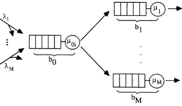
The multi-class queueing network under study is a tree-like configuration consisting of a node

linked to M parallel nodes as shown in figure 1. We shall refer to the first node as node0, and the

M parallel nodes are numbered from 1 to M. Each node is represented by a single server queue

with a finite capacity b, (i=O,I, ...,M) including the space in front of the server. There are M

classes of customers. Class i customers arrive at node

0

in a Poisson fashion at a rate Ai and they

receive an exponentially distributed service with parameter Jloi (i= 1,...,M). Each class of

customers has a unique destination node. That is, upon service completion at node 0, class i

customers always join node i (i=l,...,M). In view of this, node

°

is shared by all classes, while nodes 1 to M is used only by a single class. The service times at node i (i=l,...,M) are

exponentially distributed with parameter

Jli-Figure 1: The multi-class queueing network under study

We assume that class i (i=1,2, ....M-l) has a higher priority than class i+1. The service discipline

at node 0 is head-of-line with pre-emption. Note that since the service times are exponentially

distributed and because of the memoryless property of the exponential distribution, it is not

important to specify whether the discipline is pre-emptive resume or pre-emptive repeat.

Due to the fact that the destination nodes I to M are finite, the flow of customers through node0

may be blocked. Blocking-before-service is assumed (see [6]). That is, a customer cannot begin

his service unless there is space in the destination node. Ifnode i becomes full upon service

completion at node 0, the whole class i of customers becomes blocked. However, the server at

node 0 is not blocked, and it can proceed to serve customers from lower classes that may be

present at node

O.

The server will become blocked if all classes present at node

0

are blocked.

Class i becomes unblocked at the moment when a departure takes place from node i (i=1,2,...,M).

Due to service pre-emption, a class i customer can start service immediately, if the server is busy

serving a lower class customer. We shall refer to thistype of blocking as class blocking. We note that in view of this type of blocking, it is possible to have a lower class customer in service while higher class customers are present at node

0

despite the service pre-emption discipline. This

happens when all the higher class customers are blocked.

Blocking-before-service has been used extensively in single-elass queueing networks with finite

capacity queues. The difference between this blocking mechanism and the class blocking

mechanism described above, is that in the former case the server gets blocked each time a customer

becomes blocked. Intuitively speaking, one can easily see that under the class blocking

mechanism, the utilization of the server at node

0

is higher than in the case of blocking before

service, and therefore the system's throughput is also higher.

The overall capacity of node 0, b

o,

is shared by all classes of customers. Unlike other finite

capacity nodes, a customer that arrives to node 0 when the node is full, is not always lost. In

particular, let us assume that a class i customer arrives when node

0

is full. Then, the customer is

lost if the node at that moment only contains customers of class i or higher. However, if the node

contains lower class customers, then a customer of the lowest class currently present at node0is

forced out of the node so that the arriving customer may enter the node. As an example, let us

consider the case where we have four classes (i.e. M

=

4). Let us assume that node 0is full and that a class2 customer arrives. The customer will get lost if node 0 at that moment only contains

or class 4 customer present. In particular, the arriving customer will frrst attempt to force out a

class 4 customer. If there is no class 4 customer present, then he will force out a class 3 customer.

In general, when the arriving class i customer forces a class j customer out of node 0 (where

j > i), the forced out customer within class j is the one that arrived last. Due to the service

pre-emption discipline, this customer will be forced out even if at that moment it so happens that he is

receiving service. This mechanism for managing the space in a finite capacity queue is known as

push-out.

This mechanism and other similar mechanisms have been proposed within the context of high-speed computer networks. However, only two classes have been considered (see [3]).

3.

The approximation algorithm

In this section, we present an approximation algorithm for analyzing the multi-class queueing

network with blocking described above. We analyze this queueing network using a single-node

decomposition algorithm. The principle of this algorithm is similar to that proposed in [7] for

single-class queueing networks with blocking-after-service. The multiclass queueing network

described in section 2 is analyzed by decomposing it to its individual nodes. In particular, each

node i is analyzed by approximating it by another node, hereafter referred to as Qi (i=O,l ....,M).

Q

_i (i=l,...,M) is a single-class node with the same buffer capacity and service rate as node i but

with a revised arrival process. This arrival process approximates the actual arrival process to node i

from node

0

in the original network. This arrival process is assumed to be Poisson with rate Ai.

Thus,

Q

_i is simply an MIM/l/N queue with arrival rate ~i' service rate ~i' and buffer capacity b.. Let Pi(~) to be the steady-state probability that there are k,customers in Qi(~=O,l ,....b.) and let Xi be the throughput of Qi. For a given arrival rate Ai, these quantities can be easily calculated.

Qo is a multiclass node that is identical to node

0

except that the blocking effect due to the

downstream nodes (nodes 1 to M) is taken into account in an approximate way. The blocking

effect is modelled as follows. Upon service completion of a class i customer at Qo, class i is

blocked with a probability ri and is not blocked with a probability I-ri. If it is blocked, the server is

prevented from servicing class i customers. This blocking condition will last for a period of time

that is exponentially distributed with rate Jli. As soon as this period of time ends, the server is again allowed to serve customers of class i. Due to service pre-emption, a class i customer can start

otherwise identical to that of node 0, i.e. it has the same service priority and space priority

mechanisms. Let PO(nOi) denote the probability that there are nOi class i customersin Qo. Also, let

Xoi

be the throughput of class i customers at Qo.Note that X_{Oi is less than} Ai due to the finite capacity of

Qo

and also due to push-out.

The behavior of

Q

o

can be described by a continuous-time Markov chain (CTMC). The state of

this CTMC is defined by the vector s = (n1,jl, ... ,ni,ji, ...,nM,jM). ni is the number of class i

customers currently present at

Q

o

(ni=O,1,...,b

o)

and ji is a parameter that indicates whether class i is blocked or not. ji

=

°

if class i is not blocked and ji

=

1 if class i is blocked. Let Q be the infinitesimal generator of the CTMC of

Qo.

Let P be the stationary probability vector of all probabilities of state. Then, p can be obtained by solving numerically the system of linear

equations

pQ

= 0 and

pe

= 1.

In order to analyze

Qo

we need to know the completion instant blocking probabilities ri

(i=l,...,M). Each probability ri is approximated by the probability that a customer arriving to Qi

will occupy the last position (see[2]). Let 1Tibe this probability. Then, we have

Also, the analysis of Qi (i=I,...,M) requires knowledge of the arrival rate

~i'

This arrival rate is

determined in such a way that the throughput ofQiis equal to the throughput of classi customers

in Qo, that is

Xi

=

X

Oi•

The following iterative algorithm can beused to determine the unknown parameters:

Algorithm 1.

Step

O.

Initialization.

Set X_Oi

=

Ai' for all i

=

1,2,...,M.

Step 1.

Analysis of each single-class queue Q,

For i

=

1,2,...,M :

Step l.a. Determine ~i such that Xi=X Oi'

Step

2. Analysis of the multi-class queue Qo. Step 2.a. For i

=

I, ...~ M, set ri

=

ITi' .

Step 2.b. Calculate the steady-state probability vector p. Step 2.c. For i

=

1...., M, deri ve the throughputs X_Oi•

Step 3.

Go to Step I until convergence of the unknown parameters.

Step

4. Calculate all performance measures of interest.

Algorithm I is an iterative procedure that analyzes the set of single-class nodes Qi (i=1,2....,M)

and the multi-class node Qo in tum. On the one hand, for given values of the throughputs, Step 1

calculates new values of the blocking probabilities1Tio In Step l.a, the value ofAiis obtained as the

solution of the fixed-point iteration: ~i

=

_{Xi I(l-Pi(bi)) (see [2], and [7] for details). On the other}

hand, for given values of the blocking probabilities, Step 2 calculates new values of the throughputs

Xoi.

In Step 2.b, the vector p is the solution of the system of equations pQ=

0

and

pe= 1. In our implementation of this algorithm, we used the power method to solve the above system of equations. Obviously, more efficient methods can be used (see [10]). In Step 3, the iterative procedure is stopped as soon as (1Ti(k)-1Ti(k-l»)I1Ti(k) < e, for all i=l,...,M, where JTi(k)is

the k-th estimate ofITi. In our implementation of this algorithm, we used e

=

10-5•

In terms of complexity, the main difficulty of algorithm 1 lies in the numerical solution of the CTMC associated with Qo. The cpu and memory complexity of the solution depends on the size of

the state space of the CTMC. The number of states of the CTMC is a function of the buffer

capacity bo of Qo and the number of classes of customers M. Thus, the size of the CTMC is very large when bo and M are large. Moreover, the CTMC has to be solved as many times as the

number of iterations required for the convergence of algorithm 1. Thus, this numerical solution can

only be used when the CTMC associated with Qo is of moderate size. In the next section. we

present an approximation method for analyzing Qo which avoids the complexity issues of the

above numerical solution.

4.

Class aggregation

As stated above, the size of the CTMC associated with Qo can be very large for networks with an arbitrary number of classes. However, for networks with only two classes, the number of states

solution of the CTMC associated with a network consisting of only two classes is obtainable in a reasonable amount of time.

Based on this observation, we propose a

class aggregaiion

technique which reduces the analysis of

Qo to analyzing this node M-l times, but each time with two classes of customers. Due to the

head-of-line pre-emptive service priority and the push-out mechanism, the behaviour of classi is

not affected by the lower priority classes. Thus, it can be analyzed without considering the lower

priority classes. The behavior of class i, however, is affected by the higher priority classes. In

view of this, we analyze the behavior of classi by ignoring classes i+ 1 to M, and representing all

higher priority classes i-I to 1 by a single aggregate class. Let Al._i-1denote this aggregate class.

The class aggregation technique works as follows. We first consider classes 1 and 2. Using

algorithm 1, we analyze nodes Qo, QI and

en

assuming that Qo consists of only two classes, i.e.

classes 1 and 2.Based on the results obtained, we aggregate classes 1 and2 into the single class

Al.~. We then use algorithm 1 to analyze nodes Qo and Q3, assuming that

Qo

consists of classes

AI,:!and 3.Class AI:! and class 3are then aggregated into the single class A1._3.Using algorithm 1

we analyze class nodes Qo and Q4, assuming that Qo consists of classes A1.₃and 4. We continue

in this fashion until we analyze all classes.

We now proceed to describe how two classes are aggregated into one. We first consider the

aggregation of classes 1 and 2. After algorithm 1 has been applied to nodes Qo, Ql and

en,

the quantities rl and r:! as well as the steady-state probabilities of the CTMC associated with

Q

o

are

known. Let E be the set of states of the CTMC, where each state is given by the vector (n.,jl' n:!,

j:!). E is partitioned into several subsets of states. Let E(nA' jA) be a subset of E, where

nA=O, l,...,b

o,

_{and jA=O, 1. The set of states that belong to E(n A, jA) is defined as follows:}

That is, a state belongs to E(nA' 0) if the total number of customers of classes I and2is equal to

n and one class of customers (either class 1 or 2) is currently receiving service. On the other

hand, a state belongs to E(nA' 1) if the total number of customers of classes 1 and 2 is equal to nA

and neither class 1 nor class 2 is receiving service. This happens when for each class of

customers, either there is no customer (n, = 0) or the class is blocked

Ui

= 1).It is easy to check. that the total numberofsubsets is equal to 2b

o

+1(subsetE(O, 0) is empty).

The reason we partition the states of the CfMCin this way is because the behavior of class3 in

Q

o

with respect to higher priority classes 1and 2, is only affected by two factors: 1) the total

number of class 1and 2 customers currently present in Qo, and 2) whether the server is busy

working on aclass I or2customer. The former factor is represented by variable nA and the latter

by jA.

According to this partition, we can define

an

aggregate CTMC. Each state of this aggregate CTMC

is given by the vector (n_{A ,}jA), and the total number of states is equal to the number of subsets of

states of the original CTMC. The transitions rates are obtained using standard Markov chain

aggregation. Let us briefly recall how this works. Consider a CTMC partitionned into several subsets of states

{E1,...

,E;.,...

,E_{R } .} Letj be any state of the CTMC and let pU) be the probability of being in state j. Let

YU,

k) be the transition rate between states j and k.Then, the transition rate between statesE,and E,in the aggregate CTMC, say ~(r, s), is as follows

~(r, s) =

L

(p(j)

L

y(j,

k))

jE~ kE~

The aggregate CTMC describes the behaviour of the aggregate class AI.:!. We note however that

the behaviour of the aggregate CTMC is only an approximation to the behavior of the original

CTMC. This is because the transitions between subsets of states in the original CTMC are not

Markovian.

Having aggregated classes 1 and 2 to class A1,2, we can proceed to analyze class 3. This is achieved by analyzing nodes Qo and Q3 using algorithm 1 and assuming that Qo has two classes,

namely, aggregate class Al,2 and class 3. The unknown parameters are the completion instant

blocking probabilitiesf3 of class3 customers at Qo,and the arrival rate ~3atQ3. For a given value

of r3'

Q

o

can again be analyzed by constructing a CTMC describing its behavior in a similar way

as what was done in section 3. The state of this CTMC is defined by the vector

S

=

(nA, jA' n3' j3)· The transition rates of this CTMC are obtained as follows. For any transition related to the aggregate class, i.e. any transition that involves a modification of either nA

orjAor both, the transition rate is obtained from the aggregate CTMC described above. For any transition related to class 3 customers, the transition rate is simply obtained according to the

Markovian behavior of class

3.

The unknown parameters, f3 and A3' can then be determined using a fixed-point procedure similar to that described in algorithm 1. Having analyzed class 3,classes Al,:! and 3can be aggregated

into the single class A_{t 3}in a similar way as describe above for classes 1 and 2. The behaviour of class A_{I .3 is thus described by an aggregate CTMC whose transition rates are obtained from the}

steady-state probabilities ofQo. Class 4 can be analyzed using algorithm 1 for the nodes Qoand

Q4'and assuming that Qohas two classes, namely, class A_t,3and 4. This procedure is repeated

until all classes have been analyzed.

The main steps of this approximation algorithm are summarized below.

Algorithm 2.

Set i

=

1.

Step O. Initialization

Set XOi

=

Ai·

Step 1. Analysis of Qi.

Step l.a. Determine~i such that Xi

=

XOi•

Step l.b. Calculate the probabilityITi·

Step 2. Analysis of

Q

o

consisting of class A1,i-l and class i,

Step 2.a. Set ri

=

Tri·

Step 2.b. Calculate the steady-state probability vector p. Step 2.c. Derive the throughput XOi•

Step 3. Go to Step I until convergence of the unknown parameters.

Step 4. Derive the transition rates of the aggregate class Al.i ·

5. Validation

The approximation algorithm described above, including the class aggregation approach, was.

implemented on a vax workstation. Different configurations were analyzed and the approximate

results were compared against simulation data. The simulation model was developed using

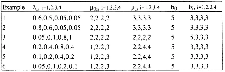
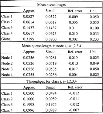
QNAP2 [9].Six representative comparisons between the approximate and the simulation dataare

presented in tables2to7assuming4classes of customers. Each table gives the mean queue length

for each class in node 0, the global mean queue length for node 0, the mean queue length for

nodes 1 to 4, and the throughput of each class (departure rate from queue 1, 2, 3, and 4). The

relative error calculated as (simul-approx)/ simul is also given. In general, the accuracy of this type

of approximation algorithm depends upon the amount of traffic carried by the network. Therefore,

in order to put the results in perspective, each table gives the utilization, as measured by

simulation, of the server at node

°

(per class and global), and the utilization of the servers at nodes 1 to 4. The parametersof the six examples are given in table 1.

Example Ai, i=1,1,3,4 J..L0i, i=1,2,3,4 Ili, i=1,1,3,4

bo

bi, i=1,2~3,4

1 0.6,0.5,0.05,0.05 2,2,2,2 3,3,3,3 5 3,3,3,3

2 0.8,0.6,0.05,0.05 2,2,2,2 3,3,3,3 5 3,3,3,3

3 0.05,0.1,0.8,1 2,2,2,2 2,2,2,2 5 5,3,3,3

4 0.2,0.4,0.8,0.4 1,2,2,3 2,2,4,4 5 J,3,3,3

5 0.1,0.2,0.4,0.2 1,2,2,3 2,2,4,4 5 3,3,3,3

6 0.05,0.1,0.2,0.1 1,2,2,3 2,2,4,4 5 3,3~3,3

Table 1: Parameters of the examples given in tables 2 to 7

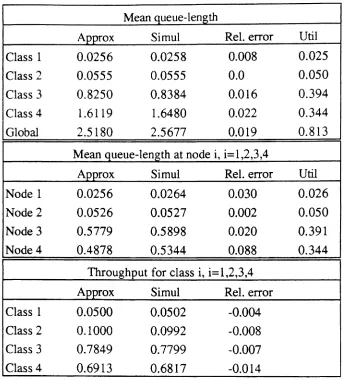
Tables 2 and 3 give results where the server at node

°

is utilized considerably more by classes 1

and 2than by classes3and 4. The utilization of the server at node

°

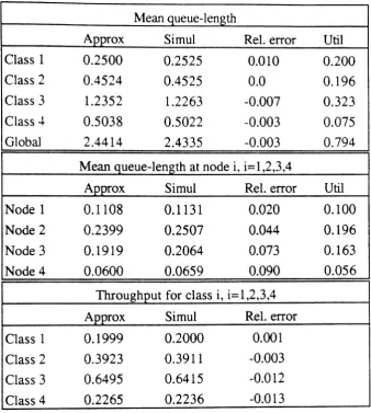
is about58% in table 2and about 70% in table 3. Table 4 gives an example where the utilization of classes 3 and 4 is higher

than the utilization of classes 1 and 2, and in the example given in table5 the utilization of class3

is higher. The server's utilization at node 0 is about 81

%

in table 4 and 79% in table 5. The

examples given in tables 6and 7 are for two cases where the utilization of the server at node0 is

lower than in the four previous examples, i.e. about 45% and 23% respectively. We note that the

approximation algorithm performs well and, in general, the relative errors are quite low.

6. Conclusions

One of the main difficulties encountered when analyzing approximately open queueing networks

with blocking, is the analysis of a single node. Due to multiple classes and blocking, this is not a

simple task as it was in the case of single-class open queueing networks with blocking. In this

paper, we considered an open multi-class queueing network consisting of a finite capacity node

(node0) linked to M parallel finite capacity nodes (nodes 1 to M). Of interest in this paper, was the analysis of node

0

for which we assumed M classes of customers, head-of-line with

pre-emption service priority, blocking, and a mechanism for managing the space in node 0 known as

push-out. This queueing network is analyzed approximately using single-node decomposition. The

computational complexity of analyzing node

0

numerically increases rapidly as the number of

classes increases.

In

order to avoid this problem, we proposed a class aggregation technique which

avoids the complexities of the numerical technique. The approximation algorithm has been

Mean queue-length at node0

Approx Simul ReI. error Dtil

Class 1 0.4298 0.4160 -0.033 0.304

Class 2 0.6292 0.6049 -0.040 0.236

Class 3 0.0764 0.0753 -0.015 0.022

Class4 0.0781 0.0803 0.027 0.022

Global 1.2135 1.1765 -0.031 0.584

Mean queue-length atnode i, i=1,2,3,4

Approx Simul ReI. error Util

Node 1 0.2450 0.2464 0.006 0.200

Node2 0.1864 0.1954 0.046 0.159

Node 3 0.0148 0.0149 0.007 0.015

Node4 0.0144 0.0142 -0.014 0.014

Throughput for class i, i=1,2,3,4

Approx Simul ReI. error

Class 1 0.5989 0.5982 -0.001

Class 2 0.4751 0.4696 -0.012

Class 3 0.0437 0.0425 -0.028

Class 4 0.0427 0.0422 -0.012

Table2: Example 1.

Mean queue-length

Approx Simul ReI. error Util

Class 1 0.6611 0.5958 -0.109 0.398

Class 2 0.8900 0.8470 -0.051 0.262

Class 3 0.0826 0.0824 -0.002 0.018

Class 4 0.0829 0.0806 -0.028 0.017

Global 1.7166 1.6058 -0.070 0.695

Mean queue-length at node i, i=I,2,3,4

Approx Simul Rei. error Uill

Node 1 0.3465 0.3486 0.006 0.265

Node 2 0.2089 0.2244 0.069 0.176

Node 3 0.0123 0.0121 0.017 0.012

Node 4 0.0119 0.0119 0.0 0.012

Throughput for class i, i=1,2,3,4

Approx Simul Rei. error

Class 1 0.7946 0.7888 -0.008

Class 2 0.5238 0.5222 -0.003

Class 3 0.0365 0.0362 -0.028

Class 4 0.0351 0.0351 -0.023

Mean queue-length

Approx Simul ReI. error UtiI

Class

1

0.0256

0.0258

0.008

0.025

Class 2

0.0555

0.0555

0.0

0.050

Class

3

0.8250

0.8384

0.016

0.394

Class

4

1.6119

1.6480

0.022

0.344

Global

2.5180

2.5677

0.019

0.813

Mean Queue-length at node i,

i=1,2,3,4

Approx Simul ReI. error Util

Node

1

0.0256

0.0264

0.030

0.026

Node

2

0.0526

0.0527

0.002

0.050

Node

3

0.5779

0.5898

0.020

0.391

Node

4

0.4878

0.5344

0.088

0.344

Throughput for class i,

i=I,2,3,4

Approx Simul ReI. error

Class

1

0.0500

0.0502

-0.004

Class 2

0.1000

0.0992

-0.008

Class

3

0.7849

0.7799

-0.007

Class

4

0.6913

0.6817

-0.014

Table 4: Example

3.

Mean queue-length

Approx Sirnul ReI. error Util

Class I 0.2500 0.2525 0.010 0.200

Class 2 0.4524 0.4525 0.0 0.196

Class 3 1.2352 1.2263 -0.007 0.323

Class 4 0.5038 0.5022 -0.003 0.075

Global 2.4414 2.4335 -0.003 0.794

Mean queue-length at node i, i=I,2,3,4

Approx Simul ReI. error Util

Node 1 0.1108 0.1131 0.020 0.100

Node 2 0.2399 0.2507 0.044 0.196

Node 3 0.1919 0.2064 0.073 0.163

Node 4 0.0600 0.0659 0.090 0.056

Throughput for class i, i= 1,2,3,4

Approx Simul ReI. error

Class I 0.1999 0.2000 0.001

Class 2 0.3923 0.3911 -0.003

Class 3 0.6495 0.6415 -0.012

Class 4 0.2265 0.2236 -0.013

Mean queue-length

Approx Simul ReI. error UtiI

Class 1 0.1111 0.1071 -0.037 0.097

Class 2 0.1520 0.1481 -0.026 0.098

Class 3 0.4124 0.3939 -0.048 0.195

Class 4 0.2032 0.1972 -0.030 0.063

Global 0.8787 0.8463 -0.038 0.453

Mean queue-length at node i, i=1,2,3,4

Approx Simul ReI. error Util

Node 1 0.0526 0.0510 -0.031 0.048

Node 2 0.1107 0.1112 0.004 0.099

Node 3 0.1086 0.1098 0.011 0.097

Node 4 0.0493 0.0516 0.045 0.048

Throughput for class i, i=1,2,3,4

Approx Simul ReI. error

Class 1 0.1999 0.2000 -0.032

Class 2 0.3923 0.3911 -0.017

Class

3

0.6495 0.6415 -0.016

Class 4 0.2265 0.2236 0.001

Table

6:

Example 5.

Mean queue-length

Approx Simul ReI. error Uti1

Class 1 0.0527 0.0522 -0.009 0.050

Class 2 0.0614 0.0618 0.006 0.050

Class 3 0.1437 0.1437 0.0 0.100

Class 4 0.0617 0.0623 0.010 0.033

Global 0.3195 0.3200 0.002 0.233

Mean queue-length at node i,i=1,2'l3,4

Approx Simul ReI. error Util

Node 1 0.0256 0.0261 0.019 0.025

Node 2 0.0526 0.0519 -0.013 0.049

Node 3 0.0526 0.0535 0.017 0.050

Node 4 0.0255 0.0256 0.004 0.025

Throughput for class i, i=1,2,3,4

Approx Simul ReI. error

Class 1 0.0500 0.0494 -0.012

Class 2 0.1000 0.0989 -0.011

Class 3 0.1998 0.1975 -0.012

Class 4 0.0996 0.0989 -0.007

References

[IJ

[2]

[3]

[4]

I. Akyildiz and H. G. Perros (Eds.),

Special Issue on Queueing Networks

with

Finite

Buffers,

Performance

Evaluation,

Vol. 10, pp. 197-210, 1989. .

Y.D~llery and Y.Frein,On decomposition methods for tandem queueing networks with

blocking, Tech. Rep. MASI No. 293, Universite Pierre et Marie Curie, July 1989.

A.A. Nilsson, F. Lai, and H.G. Perros, Aqueueing model of a bufferless synchronous Clos ATM switch with head-of-line priority and push-out, Tech. Rep. 90-18, Computer Science Dept., North Carolina State University, 1990.

R. O. Onvural, A survey of closed queueing networks with finite buffers, ACM

Computing Surveys,

Vol. 22. No 2, pp. 83-121, 1990.

[5] R. O. Onvural and H. G. Perros, Approximate analysis of multi-class tandem open

queueing networks with Coxian parameters and finite buffers, King, Mitrani, Pooley (Eds.) Performance '90(North-Holland, 1990) 131-141.

[7]

[8]

[9]

[6]

H. G. Perros, Open queueing networks with blocking, Stochastic Analysis of Computer

and Communication Systems, Takagi (Ed.), North Holland, 1989.

H. G. Perros and T. Altiok, Approximate analysis of open queueing networks with blocking: tandemconfigurations,

IEEE Transactions on Software Engineering,

Vol

SE-12, N°3, pp. 450-461, 1986.

H. G. Perros and T. Altiok (Eds.), Proc. of the First Int. Workshop on Queueing

Networks with Blocking, North Holland, 1989.

QNAP2, Reference manual, version 4.0, Simulog, Av. du Centre, 78182 St. Quentin en

Yvelines, France.

[10] W. J. Stewart, A comparison of numerical techniques in Markov modeling,

Communications ofthe ACM, Vol. 21, N°2, pp. 144-152, 1978.