ABSTRACT
SHAVER, KAY ALBRIGHT. Activity-based Evaluation of Operations
Management within Service Operations Organization. (Under the direction of John Dutton.)
The purpose of this study is to use historical cross-sectional data
including order characteristics to predict the time requirements of the indirect activity of managing. The subject of the study is the Operations Manager, who manages the supervision of engineering and installation of orders. Predictions of time estimates for the Operations Manager will provide information for staffing and workforce planning of the indirect activities required to manage the forecasted order workload.
The research includes a pilot survey of Operations Managers in three regions and a final empirical study, which includes the entire Service
Organization’s Operations Manager population. Using regression analysis, the study evaluates the factors noted in the pilot survey as important to the
Operations Managers. Consideration is given to order characteristics, such as size, customer relationships, schedule changes, interval, Operations Manager assigned. Consideration is also given to general characteristics, such as seasonal effects, concurrent orders, experienced installers available, and inventory levels. The analysis reveals that category of work, size of the order as measured by number of frames, seasonal impacts, the Operations Manager assigned, customer relationships, and the effort required to underspend the budget are key
Personal Biography
The author is a native of North Carolina and a 1986 graduate from the
University of North Carolina at Chapel Hill with a Bachelor of Science degree in Business Administration. Immediately after graduating from the University, Ms Shaver joined a large manufacturing firm located in the Research Triangle Park where she is currently a Senior Manager. After several years working at the firm, Ms Shaver pursued a Master of Arts in Economics from North Carolina State University focusing on economic practices as well as the international environment. Ms Shaver applied these learning’s to the business environment– specifically in activity-based models for resource planning. This thesis
TABLE OF CONTENTS
Page
List of Tables v
List of Figures vi
List of Abbreviations vii
1.0 Introduction 1
2.0 Literature Review 3
3.0 Sub problem #1 - Pilot Survey of OM Activity 7
3.1 Survey Content 7
3.2 Survey Results 8
3.2.1 Experience / education / background (Page 2) 8
3.2.2 Comfort level (Page 3-4) 8
3.2.3 Workload and mix (Page 5) 9
3.2.4 Factors influencing Operations Manager activities
(Page 5-6) 11
3.2.5 Weekly activities / hours worked (Page 7) 12
3.3 Topic Evaluation and Availability 15
3.4 Transforming Survey Data into a Forecast 16
4.0 Sub problem #2 - Final Empirical Study of OM Activity 18
4.1 Data Collection and Preparation 19
4.2 Regression - Model Refinement and Selection 23
4.2.1 Model A- 136 DF 23
4.2.2 Model B - 86 DF 24
4.2.3 Model B Residual Analysis 28
4.2.4 Model B Log Restricted 30
4.3 Evaluation/Validation of Final Regression Model 33
6.0 Summary of Significant Findings 42
7.0 Recommendations for Further Research 45
8.0 List of References 47
9.0 Appendices 49
9.1 Survey / Survey mapping of Question #7 50
9.2 Cumulative Operations Manager Variable 58
9.3 Mapping to Category 59
9.4 Dataset Reports / Plots 65
9.5 Regression Results - Model A 79
9.6 Regression Results - Model B 85
9.7 Regression Results - Model C 92
LIST OF TABLES
Page SUB PROBLEM #1 -PILOT SURVEY OF OM ACTIVITY
3.1 Survey Results: Workload 11
3.2 Survey Results: Impacting Factors 12
3.3 Survey Results: Hours Per Week by Activity 13
3.4 Survey Results: Summary Hours By Operations Manager 14
3.5 Impacting Variable 16
SUB PROBLEM #2 - FINAL EMPIRICAL STUDY OF OM ACTIVITY
4.1 Model Independent Variables 19
4.2 Model A-2 - Group Test Results 24
4.3 Pearson Correlation Results (Model B) 26
4.4 Multicollinearity Subset Testing 27
4.5 Results of Log Transformation With Previous
Best Fit Models 30
LIST OF FIGURES
Page LITERATURE REVIEW
2.1. Strategy for Building a Regression Model 6
SUB PROBLEM #1 - PILOT SURVEY OF OM ACTIVITY
3.1. Pilot Survey Results: Comfort Levels & Experience 9
3.2. Job Categories 10
3.3. Operations Manager Activity System – Overview 17
SUB PROBLEM #2 - FINAL EMPIRICAL STUDY OF OM ACTIVITY 4.1. Operations Manager Activity System - Historical Data and
Predictions 18
4.2. Model B Log Step History 31
4.3. Model B Log Restricted vs. Model B Log Unrestricted 31
4.4. Studentized Residuals - Model B Log Restricted 32
NEXT STEPS: PREDICT OPERATIONS MANAGERS REQUIRED
5.1. Operations Manager Activity System - Staffing Process 40
LIST OF ABBREVIATIONS
OM operations managers responsible for completing the Engineering
and Installation of company hardware, software, and firmware for configuration into the customer's telecommunications network; responsible for meeting per job cost targets and customer
satisfaction; manage day - to - day activities of workforce assigned to workload by resource agency
Installation
activity performed by skilled field technicians to ensure hardware, software, and firmware are operational and functional in the customer network; physical hardware building and connecting; testing of software features and training of customers on new equipment
Engineering
provisioning network equipment; configuring new equipment into existing network; identifying hardware and software order
components; outlining interdependencies and additional order items; updating office records
EAE equipment application engineer responsible for part identification to manufacturing
Site team leader/Supervisor
site team leader or supervisor is responsible for on site management of job during Installation interval
Work in progress or Mix
number and type of jobs that an Operations Manager is assigned at one time
Potential Variables
1.0 Introduction
Executive decision making in a large organization creates the need for a systematic approach to understanding the variables that drive activities and their costs. The challenge is to evaluate the organization by activity and provide a tool for decision making using existing information. This is a study of a
service organization within a large telecommunication firm and focuses on the activity of Operations Management.
Generally speaking, the service operations organization is decentralized and operates as a cost center, with the exception of the training facility, which is a profit center. The purpose of the organization is to engineer and install telecommunication products on a per order basis. Fifty-one Operations Managers directly manage the order activities.
Making decisions within this large organization of over 2500 employees has become increasingly difficult as the product mix, market, and job characteristics change. In the absence of complete data and impact analysis, many decisions are made from gut feel, experience, and best. Often the strategy team is unable to determine if particular results were caused by a specific critical decision or by other factors. This uncertainty about causation, as well as general organizational complexity and rapidly changing conditions, greatly complicate executive
• Do we have the right number of Operations Managers in our business structure?
• When should we hire / re-deploy Operations Managers?
This study isolates the OM activity within the organization and creates a model to predict the appropriate number of OMs required to support the forecasted workloads. This study is divided into two sub problems:
1. Pilot survey of OM activity
2. Final empirical study of OM activity
The pilot survey captures qualitative information of how several variables affect the activity of OMs. OMs are responsible for managing the Engineering and Installation of customer orders, managing people, and leading strategic initiatives.
The final empirical study uses the pilot survey information to build a model to predict the number of hours an OM requires to manage each customer order. The model uses characteristics of the order, such as difficulty of work, season, OM, location, customer, and size along with other observed data, such as material availability, reschedule activity, and installation skill levels.
2.0 Literature Review
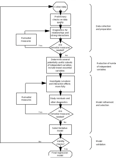
This section examines model development to forecast OM needs. The model uses a number of explanatory variables to predict how many OM hours are required for specific activities. We use linear regression to estimate statistically the effect of each variable on activity requirements. The basic steps of model building are outlined below and reproduced in the flow chart in Figure 2.1: Strategy for Building a Regression Model:
1. Data Collection and Preparation
2. Reduction of the Number of Independent Variables 3. Model Refinement and Selection
4. Model Validation1
This method has been used to predict outcomes such as economic indicators, grades of students, hog prices, sales, crop yields, and stock market performance.
Candidate variables in this study were identified in the pilot survey as
engineering resources, order characteristics, installation training, underspending against projected hours, customer relationships, organizational structure, tools, quality of products, OM comfort levels, and OM experience. The variables were reduced based on availability of information, changes in the information during the data capture period, and variable perfect collinearity. The resulting model was evaluated for group significance, heteroskedasticity, multicollinearity, and outlier influences and adjusted to produce a model that predicts the cumulative hours required by an OM to manage a customer order.
1
Studies completed by accounting researchers were reviewed, but did not provide insight for predicting the indirect OM activity of this study. The
Accounting studies focused primarily on Activity-based and Contribution-based Accounting using trend estimates of overhead cost increased periodically by inflation factors to predict indirect components of the cost of goods sold. Other studies created models using the gap between the actual revenues and the potential revenue2 along with re-engineering concepts.
A study in the field of Urban Economics by W.W. Recker and R. Ketamuran (1985), predicting urban transportation requirements and growth, did focus on the indirect activity of travel decisions through econometric modeling and simulations. Three approaches were compared in the study:
1) statistical classification of daily trips using nine behavior patterns and a technique of space/time and activity/time continuum transformation and cluster analysis,
2) preplanning assumption with simulations of travel behaviors of travel decision makers, and
3) sequential trip chaining assuming each trip made was unique and self-contained, using history and regression analysis.
Each of these approaches and results were discussed with varying degrees of author confidence for policy changes based on this analysis. 1) Statistical modeling of behaviors represented 8% of the population overall, but was
extremely accurate at peak hours of travel in local areas of work and home (three to seven miles) thus allowing policy makers to use this indirect modeling
approach. 2) Using a decision-making simulation model of preplanning
updating the input after a policy change and constantly changing behaviors of the constraints assumed in the simulation. 3) Trip Chaining, with measures of time of day, socioeconomic attributes, and duration, established regression modeling of four areas (shopping, personal business, social-recreation, serve passengers) with all models significant and explaining 8.7% - 15.9% of the variability in trip chaining. Trip Chaining remained the simplest and most convenient method of predicting trip changes in the population, but the simulator was the best predictor.3
The travel study closely matched the characteristics of the OM study and provided methodology and targeted results for comparison. Data
characteristics, such as cross sectional data and indirect activities, were similar between the two studies.
Using the travel study results and the caution by the researcher of the resources required to achieve 63% accuracy of option 2, we elected to follow the
methodology discussed in option 3 with one regression model, targeting the simplest and most convenient method for predicting OM hours.
3
W.W. Recker and R. Kitamura, “Activity-based Travel Analysis,” in
Pr elim inary checks on data
quality
Ar e r em edial m easur es
needed? C ollect data
D iagnostics for relationships and str ong inter actions R em edial
m easur es
D eter m ine sever al potentially useful subsets of independent var iables; include know n essential
var iables
Investigate cur vatur e and interaction effects
m ore fully
R em edial
m easur es Study r esiduals and other diagnostics
Ar e r em edial m easur es
needed?
Select tentative m odel
Validity checks?
F inal regression m odel
Y e s
No
N o
Y es N o Y e s
D ata collection and prepar ation
R eduction of num ber of independent variables
M odel refinem ent and selection
3.0 Sub problem #1 - Pilot Survey of OM Activity
Collection of the activity-impacting variables began with a survey and an evaluation of the survey results. The pilot survey is used to help choose the model explanatory variables to predict the OM hours required to manage each customer order. This section details the survey and results.
3.1 Survey Content
The data collection stage of model development (Figure 2.1) began with a survey / interview of three Operations Managers to determine relevant variables of the Operations Manager activity (see Appendix 9.1 for survey). Three Operations Managers were selected to represent each of three geographic areas of the U.S. population. The objectives of the survey/interview were to:
• Determine typical-day activities • Define job load and mix
• Identify variables impacting Engineering job management • Identify variables impacting Installation job management
• Identify key indicators of issues for Engineering job management • Identify key indicators of issues for Installation job management • Identify characteristics impacting job management potential • Identify support activities directly supporting job management • Determine background of sample Operations Managers
The surveys were administered via telephone interviews. Questions were asked to guide discussions surrounding the Operations Manager's experience,
• OM A - Texas,
• OM B - New York, and • OM C - Illinois.
3.2 Survey Results
The results are discussed in the following six sections by survey page number.
3.2.1 Experience / education / background (Page 2)
Page two of the survey was an Interviewee Profile Sheet to capture network information, background, and Engineering / Installation indicators. Years in the telecommunications business ranged from 13 to 39 years. Surveyed Operations Managers were relatively inexperienced in managing the Engineering function but had extensive experience in managing the Installation function. Education level was approximately the same for those surveyed. Backgrounds were similar and are not considered a differentiating factor for the evaluation. An indicator variable associated with OM is identified to represent this information.
3.2.2 Comfort level (Page 3-4)
Pilot Survey: Comfort Levels & Experience
80 83
42
26 47
80
32
39 59
81
28
13
0 10 20 30 40 50 60 70 80 90
Eng
Comfort
Inst
Comfort
Yrs Exp Tel Yrs
OM A OM B OM C
Figure: 3.1: Pilot Survey Results: Comfort Levels & Experience
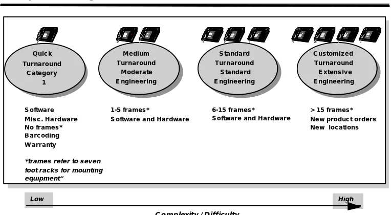
3.2.3 Workloads and mix (Page 5)
S o ftw a r e M is c . H a r d w a r e N o fr a m e s * B a r c od in g W a r r a nty
* fra m e s re fe r to s ev e n
foot r a ck s for m ounting e quipm e nt”
1 -5 fr a m e s *
S o ftw a r e a n d H a r dw a r e
6 -1 5 fr a m e s *
S o ftw a r e a n d H a r d w a r e
> 1 5 fr a m e s * N e w p r o d uc t or d e r s N e w lo c a ti on s M e di um
T ur n a r ou n d M od e r a te E ng in e e r in g Q u ic k
Tu r na r o u nd C a te g or y
1
S ta nd a r d T ur n a r ou n d
S ta nd a r d E ng in e e r in g
C u s tom i z e d T u r n a r o un d E x te n s iv e E n gi ne e r in g T he Jo b C at e g o rie s
C o m p lexit y / D if f icu lt y
Low H igh
Figure 3.2: Job Categories
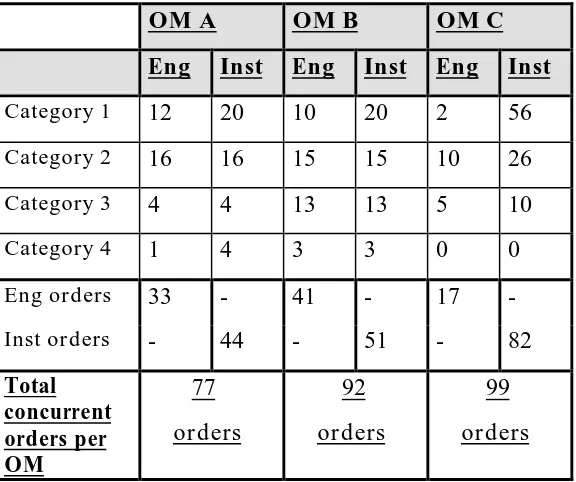
Table 3.1: Survey Results: Workload
OM A OM B OM C
Eng Inst Eng Inst Eng Inst
Category 1 12 20 10 20 2 56
Category 2 16 16 15 15 10 26
Category 3 4 4 13 13 5 10
Category 4 1 4 3 3 0 0
Eng orders 33 - 41 - 17
-Inst orders - 44 - 51 - 82
Total concurrent orders per OM
77 orders
92 orders
99 orders
Engineering and Installation Job Count by Category
3.2.4 Factors influencing Operations Manager activities (Page 5-6)
Table 3.2 Survey Results: Impacting Factors
OM A OM B OM C
Factors Eng Inst Eng Inst Eng Inst
available resources X X X
training requirements reduce hours available
X X
underspending of project
X
Engineering errors X X X X
multiple reschedule of jobs
X X
test equipment available
X
customer relationship
X X X
material shortages X X
Eng. organizational structure
X
project mgrs/site team leader (supervisors)
X X
quality audits / product quality
X
customer coverage X
customer changes X X
X indicates occurrence of item in interview - positive or negative
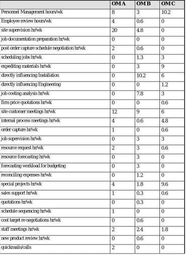
Table 3.3 Survey Results: Hours Per Week by Activity
OM A OM B OM C
Personnel Management hours/wk 8 3 10.2
Employee review hours/wk 4 0.6 0
site supervision hr/wk 20 4.8 0
job documentation preparation hr/wk 0 0 0
post order capture schedule negotiation hr/wk 2 0.6 0
scheduling jobs hr/wk 0 1.3 3
expediting materials hr/wk 0 3 9
directly influencing Installation
activities hr/wk
0 10.2 6
directly influencing Engineering
activities hr/wk
0 0 1.2
job costing analysis hr/wk 0 7.8 3
firm price quotations hr/wk 0 0 0.6
site customer meetings hr/wk 12 9 6
internal process meetings hr/wk 4 0.6 4.8
order capture hr/wk 1 0 0.6
job supervision hr/wk 0 3 3
resource request hr/wk 2 3 0.6
resource forecasting hr/wk 0 3 0
forecasting workload for budgeting
hr/wk
0 3 0
reconciling expenses hr/wk 0 1.2 0
special projects hr/wk 4 1.8 9.6
sales support hr/wk 1 0.3 0.6
quotations hr/wk 0 0.3 0
schedule sequencing hr/wk 1 0 0
cost target re-negotiations hr/wk 0 0.6 0
staff meetings hr/wk 2 2.4 1.8
new product review hr/wk 0 0.6 0
Hours worked were an average 61 hours per week. Responses were mapped into three groups (Appendix 9.1) and are displayed in Table 3.4:
• directly related to Customer orders,
• directly related to people management, and • directly related to other activities.
Table 3.4 Survey Results: Summary Hours By Operations Manager
Activity OM A OM B OM C
Customer order hours 40 44.4 32.4
People management hours 14 6 12
Other hours 9 9.6 15.6
Total weekly hours 63 60 60
Average hrs 61 hours/wk
Using workloads in Table 3.1 and average hours worked by OM in Table 3.4 allowed us to compute the distribution of a typical OM weekly hours as follows:
• Customer order hours 63% (39 hours)
• People management hours 18% (10.7 hours), and
• Other hours 19% (11.4 hours).
3.3 Topic Evaluation and Availability
This section of the evaluation demonstrates the second major phase of model development as noted in Figure 2.1 in Literature Review - Reduction of number of independent variables. Using the pilot survey results, we consider several areas and evaluate the explanatory value of each subject on the dependent variable–the cumulative hours required to manage an order.
As noted in section 3.2, OMs have different comfort levels with engineering and installation as well as experience. Because we do not have this data on each person and each order, we are using a categorical variable, “OM”, in the model. “Category of workload”, another indicator variable, represents complexity of the workloads in the model.
In addition to these three customer-order related variables, we’ve reviewed the items considered most imported by the OMs surveyed (pages 5-6) for inclusion in the model. Some of the factors listed in the survey are repetative; some have too little data variation to be of use; some data are unavailable.
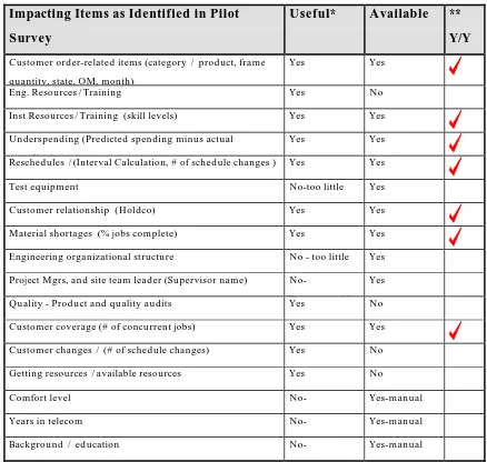
Table 3.5 lists the factors considered most important by the OMs surveyed in the pilot, the usefulness of the data, the availability of the data, and our model inclusion decision. The “Useful” column identifies those items that are represented by other variables or had too little variation during the data
Table 3.5: Impacting Variables
Impacting Items as Identified in Pilot Survey
Useful* Available ** Y/Y Customer order-related items (category / product, frame
quantity, state, OM, month)
Yes Yes
Eng. Resources/Training Yes No
Inst Resources/Training (skill levels) Yes Yes
Underspending (Predicted spending minus actual spending)
Yes Yes
Reschedules /(Interval Calculation, # of schedule changes ) Yes Yes
Test equipment No-too little
variation
Yes
Customer relationship (Holdco) Yes Yes
Material shortages (% jobs complete) Yes Yes
Engineering organizational structure No - too little variation
Yes
Project Mgrs, and site team leader (Supervisor name)
No-Represented by Yes
Quality - Product and quality audits Yes No
Customer coverage (# of concurrent jobs) Yes Yes
Customer changes / (# of schedule changes) Yes No
Getting resources /available resources Yes No
Comfort level
No-Represented by
Yes-manual collection
Years in telecom
No-Represented by
Yes-manual collection
Background / education
No-Represented by
Yes-manual collection
*“No” indicates item was either represented by another item or too little variation during data period. ** Only items with two "Yes" responses were included in model
3.4 Transforming Survey Data into Forecasts
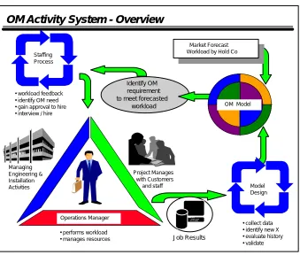
hire new staff. Figure 3.3 represents the cycle of forecasting, staffing, job managing, data collecting, and re-forecasting of the Operations Manager activity. The portion of the Operations Manager Activity System within the scope of this project is: data collection, model design, and definition of an
Operations Manager Model (order related prediction statement plus people hour estimates and non-order related hour estimates) for use with the marketing sales forecast.
Model Design Staffing
Process
OM Model Market Forecast Workload by Hold Co
Managing Engineering & Installation Activities Project Manages with Customers and staff Operations Manager
OM Activity System - Overview
Job Results
• workload feedback • identify OM need • gain approval to hire • interview / hire
• collect data • identify new X • evaluate history • validate • performs workload
• manages resources
Identify OM requirement to meet forecasted
workload
4.0 Sub problem #2 - Final Empirical Study of OM Activity
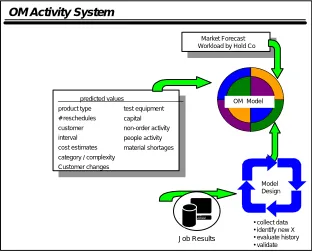
Using the useful and available factors from the pilot survey and assuming the responses were representative of the OM population, we compiled a 1995 dataset for the empirical study. Focusing on the job result variables in the Operations Manager Activity System (Figure 4.1), the dataset includes customer orders collected from week 01 to week 52 in 1995. The subsequent data evaluation relates only to customer order-related results in preparation for Operations Manager load forecasting.
OM Model Market Forecast Workload by Hold Co
predicted values product type
# reschedules customer interval cost estimates category / complexity Customer changes
test equipment capital non-order activity people activity material shortages
Model Design
• collect data • identify new X • evaluate history • validate
OM Activity System
Job Results
4.1 Data Collection and Preparation
Numerous data sources provide a cross sectional dataset of 11677 order-related records for the study. Each observation consisted of information on a particular job conducted by an OM. Observations include job-specific information plus OM characteristics, job location, etc.
Table 4.1: Model Independent Variables Pilot Survey Item Explanatory Variable Description for Model A Indicator Variable Omitted Variable
# of Explanatory
Variables in
Regression
Customer
relationship
Holdco: customer indicator for
this job
NYX 14
Customer
order-related
Month: month of active job as of
material delivery date
May 11
Customer
order-related
OM: Operations Manager
responsible for job
OM43 50
Customer
order-related
St.: State of job (includes Guam) IL 50
Customer
order-related
Cat_#: Category of work
-Appendix 9.5
Cat_2 3
Customer coverage Jobcounx: total concurrent active
installation jobs for OM
No 1
Customer
order-related
Framqty: number of frames
ordered on a job
No 1
Reschedule
-interval
Intervax: number of days job is
active
No 1
Inst Resources/
Training (skill
level)
Installx: Summary of builder,
hardware tester, operational tester,
network tester, and site team
leader competency scores
No 1
Material shortages Shortagx: percentage of material
shortages measured at first week
of installation
No 1
Reschedules RFS_ISX: Number of issues of
schedules for job
No 1
Underspending Prjdextx: Predicted costs minus
actual costs for Installation and
Engineering
Table 4.1 summarizes the independent variables of the first model as well as the characteristics of the variables: whether the variable is categorical or not, the left out category if it is, and the number of included categories for categorical
variables. As noted in Table 4.1, several variables were categorical and required transformation into indicator variables for regression analysis.
The explanatory variables of the analysis are as follows:
Frame quantity (FRAMQTY) - number of frames to install and a measure of job size,
Reschedules (RFS_ISX) - number of times a job is rescheduled,
Customer (indicator variable)- indicator variable for holding company placing the order,
State (indicator variables) - indicator variable for location of the job
Month (indicator variables) - indicator variable for month order was shipped to job location
Operation Manager (OM indicator variables) - indicator variable for OM responsible for the management of the job to proxy for OM characteristics.
Category of work (Cat_1, Cat_3, Cat_4) - an indicator variable for difficulty of workload and a summary measure of job characteristics. This variable is
to manage. The data mapping to create this variable is straight forward and the risk of introducing measurement errors is minimal.
Installation resources and skill levels (INSTALLX) - the cumulative skill of the account’s field workforce measured at two points during 1995. This variable would ideally be based on the skill level of the individuals working on a specific job, but the data did not support this level of disaggregation.
Underspending (PRJDEXTX) - predicted job costs minus actual job costs.
Predicted job costs are calculated on each job by a business analyst and provided to the OM as a budget for each order. Actual expenses are captured as time sheets are entered by engineers and installers. The difference is used in the analysis with a positive value indicating under-spending by the OM.
Material shortages (SHORTAGX) - weekly percentage of jobs shipped complete to an account. This variable would ideally be based on individual job data rather than on an aggregate weekly measure. However, the available data do not support that level of disaggregation. For example, a 57% ship complete score for week 6 for a particular customer would be used as the value for the
SHORTAGX variable for all jobs that were shipped week 6 for this account. A problem with this method is the assumption that all orders have an equal percentage of material shortages in a given week.
Job count (JOBCOUNX) - number of concurrent jobs during the first week of installation for each OM. Job Count was identified in the pilot survey as an indicator of customer coverage issues which impact the effectiveness of the OM during the installation phase of the order.
Records with missing data or data entry errors were researched and manually entered or deleted due to incomplete information. The first regression contained 11434 records and 135 explanatory variables for regression. Dataset and variable information can be found in Appendix 9.4.
4.2 Regression - Model Refinement and Selection
With the dataset defined, the research entered the third major phase of model development - Model refinement and selection (as noted in Figure 2.1 in Literature Review). During this phase, the data were evaluated for group significance and multicollinearity.
4.2.1 Model A - 136 DF
The first model, Model A, includes CUMJOBX and the independent variables noted in Table 4.1. Model A uses 136 degrees of freedom and 11434 observations resulting in a significant model with an F value of 7.732 and a p-value for the F statistic of .0001. The analysis of variance a model with an R-square of .0851, an adjusted R-square of .0741, and a root MSE of 18.65 (see Appendix 9.5 Model A).
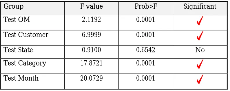
and Month are significant groups while State is not significant (see Table 4.2 for results). State is removed in the next model, Model B.
Table 4.2: Model A-2 - Group Test Results
Group F value Prob>F Significant
Test OM 2.1192 0.0001
Test Customer 6.9999 0.0001
Test State 0.9100 0.6542 No
Test Category 17.8721 0.0001
Test Month 20.0729 0.0001
4.2.2 Model B - 86 DF
Model B is then created by removing the State indicator variables. Model B uses 86 degrees of freedom and 11434 observations (see Appendix 9.6). The results indicate a significant model with an F value of 11.702 and p-value for the F statistic of .0001. Model B has an R-square of .0815, an adjusted R-square of .0745, and a root MSE of 18.64. These results are slightly better than the previous model with increases in adjusted R-square, F value, and root MSE.
Variance Inflation Factor - The VIF test creates a ratio of the actual variance of beta hat to what the variance of beta hat would have been if an independent variable was not correlated with the remaining independent variables4 . The VIF
test performed on Model B reveals significant relationships between the model variables. Comparing the relative position of the model (1/(1-R
squared))=1.08873 to the VIF and a p value of >.15 identifies relationships between a number of independent variables:
• RFS_ISX
• Jobcounx
• Intervax • Installx
• Customers 1 of 14
• Month 6 of 11
• Operations Manager 29 of 51
Of these noted above, Customer (PTL) has an inter-variable relationship as measured via VIF which is greater than five times (1.088 * 5 = 5.44365) the model relationship (see Appendix 9.6 Model B results).
Pearson Correlation - The Pearson Correlation test is a matrix which measures and displays the correlation between variable combinations. A measure of 1.0 is perfect correlation. The Pearson Correlation test confirms the results of the VIF and the presence of multicollinearity. Table 4.3 details the correlation results for all correlation’s greater than 0.30. The Pearson Correlation results identify correlation between
4
• Customer and Customer (e.g.: IND and GTE),
• Operations Manager and Customer (e.g.: OM33 and CTC), and • Reschedules (RFS_ISX) and Interval (INTERVAX).
Table 4.3: Pearson Correlation Results (Model B)
Variable Variable Correlation (+/-)
IND GTE -.32598
OM12 SPR +.71512
OM14 PAL +.36531
OM17 BST +.32204
OM18 BST +.49123
OM20 AMT +.35775
OM21 AMT +.55002
OM22 AMT +.36460
OM33 CTC +.30729
OM40 GTE +.39729
OM41 GTE +.30857
OM44 GTE +.31211
OM54 IND +.33693
OM60 PTL +.56378
OM62 PTL +.32668
OM67 PTL +.57263
OM72 PTI +.94803
OM84 BAT +.38442
RFS_ISX INTERVAX +.43585
To test the subsets as suggested by Maddala, several models are created and compared against Model B. “B-Cust (R)” is model B with all customers
restricted from the analysis. “B-OM (R)” is model B with all OMs restricted from the analysis. . “B-Cust/OM (R)” is model B with all customers and OMs
restricted from the analysis. . “B-Cust/OM/Cat/Mth (R)” is model B with all customers, OMs, categories, and months restricted from the analysis. As noted in Table 4.4, tests of subsets of variables identifies Model B as the model with the best Adj. R-sq, R-square and Root MSE. These results indicate that the
multicollinearity present in Model B is not sufficient to warrant elimination of the variable groups from the overall model.
Table 4.4: Multicollinearity Subset Testing
Model - Restricted Group DF Root MSE
R-sq Adj. R-sq F Value Prob>F
Model B 86 18.6449 .0815 .0745 11.702 0.0001
B-Cust (R) 72 18.71687 .0732 .0673 12.466 0.0001
B-OM (R) 35 18.69388 .0725 .0696 25.450 0.0001
B-Cust/OM (R) 21 18.79685 .0611 .0594 35.356 0.0001
B-Cust/OM/Cat /Mth 7 19.03796 .0357 .0351 60.361 0.0001
Eigenvalues / Variance Proportion - The final evaluation of multicollinearity is a collinearity test that produces Eigenvalues, condition values, and variance
Three data points identify sets of multicollinear variables using Eigenvalues. First, Eigenvalues of zero or near zero, indicating high degrees of
multicollinearity within a dataset, are paired with a second factor, condition values greater than 30, which identify observations with large ratios of largest to smallest Eigenvalues. Lastly, Eigenvalues that meet this criteria are evaluated for Variance Proportion Values greater than 50% identifying the proportion of the variance that is attributable to the multicollinearity. The variables meeting all three data points exhibit strong near linear dependencies and should be re-evaluated by the researcher.6
The results of this analysis on the OM activity dataset reveals one observation that meets all three of the above criteria for re-evaluation:
Obs 137
• Eigenvalue .00387
• Condition Value 48.39119
• Variance Proportion OM84 of .5182%.
With only one variable (OM84), and therefore no significant sets of variable interrelationships in the dataset, the presence of multicollinearity is dismissed as not strong enough to alter the model statement. These results were deemed not sufficient to alter Model B and it remains the best model.
4.2.3. Model B Residual Analysis
Outlier influence identification requires testing of the residual analysis using Cook’s Distance Statistic. Outliers are detected by comparing the Cook’s D to a critical F value (F crit .5, p+1, n-p-1).7 For this dataset, Cook’s D values greater
than .99 are considered significant and an indicator of outliers in the dataset. The SAS evaluations for Model B did not exhibit any Cook’s Distance Values greater than .539 after data entry errors were removed.
Heteroskedasticity of our data is another problem for us to consider. Typically, heteroskedasticity is exhibited as studentized residuals values greater than | 2.5 |, and a funnel pattern in the studentized residual plotted against the predicted values of the dependent variable. Model B exhibits this pattern and has
studentized residuals as high as | 67 |.
To determine the variables introducing the unequal error variances, we examine plots of the non-indicator variables against CUMJOBX for variables that are not in the appropriate form. Unfortunately, these were difficult to use as diagnostic indicators of curvature due to the large dataset and the numerous hidden
observations. Transformation of the independent variables was examined in another model, Model C, to see if heteroskedasticity is reduced. Model C results are listed in Table 4.5 (see Appendix 9.7 for results). Model C continues to exhibit the presence of heteroskedasticity with studentized residuals reaching | 17 |.
A log transformation of the dependent variable, CUMJOBX, is examined in another model, Model B Log, and emerges as the best fit Model. Performing a natural log transformation of the independent variable gives an F value of
7
33.9775 and studentized residuals less than |4.5|. Model B Log is adopted as the best fit for further evaluation. See Table 4.5 for Model B Log results.
Table 4.5: Results of Log Transformation With Previous Best Fit Models
Model Statement
DF Root MSE
R-square
Adj. R-sq
F Value Prob>F
Model B 86 18.6449 .0815 .0745 11.702 0.0001
Model C 90 18.4071 .1051 .0980 14.796 0.0001
Model B Log 86 1.047136 .2033 .1973 33.9775 0.0001
4.2.4. Model B Log Restricted
The final step in model refinement is to review the regression results and
Step History Step 1 2 3 4 5 6 7 8 9 10 11 12 13 14 15 16 17 18 Parameter OM80 INTERVAX INSTALLX APR OM20 OM62 BST OM11 OM64 OM30 OM53 JUL XXX SHORTAGX OM32 OM88 OM65 OM86 Action Removed Removed Removed Removed Removed Removed Removed Removed Removed Removed Removed Removed Removed Removed Removed Removed Removed Removed "Sig Prob" 0.9410 0.9125 0.8357 0.8307 0.8107 0.7803 0.6134 0.7023 0.6955 0.6872 0.6273 0.5355 0.4897 0.4822 0.4691 0.4521 0.3812 0.3134 Seq SS 0.006013 0.013233 0.047159 0.050128 0.0629 0.085307 0.279833 0.160113 0.16788 0.177709 0.258366 0.420758 0.522674 0.541058 0.57421 0.619278 0.83994 1.11312 RSquare 0.2034 0.2034 0.2034 0.2034 0.2033 0.2033 0.2033 0.2033 0.2033 0.2033 0.2033 0.2032 0.2032 0.2032 0.2031 0.2031 0.2031 0.2030 Cp 85.005 83.018 81.061 79.106 77.164 75.241 73.497 71.643 69.796 67.958 66.193 64.577 63.054 61.547 60.071 58.636 57.402 56.417 p 86 85 84 83 82 81 80 79 78 77 76 75 74 73 72 71 70 69
Figure 4.2: Model B Log Step History
Analysis of Variance
Source DF Sum of Squares Mean Square F Ratio
Model 68 3198.247 47.0331 42.9282 Error 11468 12564.600 1.0956 Prob>F
C Total 11536 15762.847 0.0000
Unrestricted model Vs. Restricted model
Summary of Fit
RSquare RSquare Adj Root Mean Square Error Mean of Response Observations (or Sum Wgts)
0.202898 0.198171 1.04672 1.619497 11537
Summary of Fit
RSquare RSquare Adj Root Mean Square Error Mean of Response Observations (or Sum Wgts)
0.203358 0.197373 1.047136 1.619811 11534
.
Analysis of Variance
Source DF Sum of Squares Mean Square F Ratio
Model 86 3204.029 37.2561 33.9775 Error 11447 12551.567 1.0965 Prob>F
C Total 11533 15755.596 0.0000
F Calculation: (12564.6 - 12551.567) / 18
1.0965
= .6603
Studentized Resid LCUMJX -3 -2 -1 0 1 2 3 Normal Quantile
-3.0 -2.0 -1.0 0.0 1.0 2.0 3.0 4.0 5.0
Quantiles maximum quartile median quartile minimum 100.0% 99.5% 97.5% 90.0% 75.0% 50.0% 25.0% 10.0% 2.5% 0.5% 0.0% 5.1469 3.1834 2.1498 1.2372 0.5828 -0.0103 -0.6390 -1.2345 -1.8960 -2.4591 -3.2325 Moments Mean Std Dev Std Err Mean upper 95% Mean lower 95% Mean N Sum Wgts -0.00 1.00 0.01 0.02 -0.02 11537.00 11537.00
Test for Normality
KSL Test
D
0.031297
Prob>D
0.0010
Figure 4.4: Studentized Residuals - Model B Log Restricted
Table 4.6: Results of Final Model with Previous Best Fit Models
Model Statement DF Root MSE R-square Adj. R-sq
F Value Prob> F
Model B 86 18.6449 .0815 .0745 11.702 0.0001
Model C 90 18.4071 .1051 .0980 14.796 0.0001
4.3. Evaluation/Validation of Final Regression Model
Validation is the process of evaluating the reasonableness of the regression results relative to the real world environment. Note that the stepwise regression process removed Installation Skills (INSTALLX), Reschedule -interval
(INTERVAX), and Material shortages (SHORTAGX) from the final model. In the following discussion, we use the pilot survey and the researcher’s knowledge of the business to discuss the parameter estimates of Model B Log Restricted.
Customer relationships (Customer)
-Final: ALL, AMT, BAT, CTC, CTY, GTE, IND, PAL, PTI, PTL, SPR, UNC. Omitted Indicator Variable: NYX
Removed: BST, XXX.
We expected that newer customer relationships would require more effort than the older established customer relationships. Older established customers are those that were deregulated in 1984 from the AT&T monopoly, such as AMT, BAT, NYX, and BST. New customers are smaller, rural, or new industry
entrants, such as GTE, SPR, XXX, ALL, CTC CTY, IND, PAL, PTI and UNC. We expected the more established customers to be removed during the stepwise regression, noting that they would require the same management time as the omitted NYX established customer. Instead, the modeling process reveals that customer relationships that are most like NYX are BST (established) and XXX (less established). XXX customers are the “other” category for undefined customers in the database and on average may be treated by OMs as an established customer. Therefore, our expectations of a simple distinction between customers is not met, and no clear pattern emerges from the data.
segmenting jobs into two orders (1-preparation, 2-equipment placement), a fact which may account for this result.
The remaining customers requiring more hours for OMs to manage than BST, NYX, and XXX are as follows:
• Orders placed by ALL, BAT, CTC, CTY, PAL, IND, and PTI customers
require from 8.6% to 11.2% more hours to manage than orders placed by BST, XXX, and NYX;
• Orders placed by SPR, UNC, and AMT customers require from 6.7% to 7.8% more hours to manage than orders placed by BST, XXX, and NYX.
Customer orderrelated (Months)
-Final: JAN, FEB, MAR, MAY, JUN, AUG, SEP, OCT, NOV, DEC. Omitted Indicator Variable: May
Removed: APR, JUL.
We expected that the order month would affect the cumulative hours required to manage a job. Specifically, we expected typical high volume quarter-bordering months–DEC/JAN, MAR/APR, JUN/JUL, SEP/OCT–to leap above the omitted MAY variable and require more effort to manage these orders. High volume is associated with revenue targets which increase engineering orders in the last month of a quarter and increase installation orders in the first month of the sequel quarter. We expected middle-of-quarter months to be similar to MAY and therefore insignificant for prediction purposes.
compared to MAY. Quarter-bordering months aligning with our expectations are:
• JAN and DEC orders, which require more hours to manage than APR, JUL, and MAY orders by 57.8% and 53% respectively.
• MAR, JUN, and OCT, which require more hours to manage than APR, JUL, and MAY by 13.8%, 8%, and 7%.
The only middle-of-quarter month meeting the expected pattern is NOV, which is insignificant. In contrast, FEB is significantly different from APR, JUL, and MAY with a positive impact (21%) on the hours required to manage a job. FEB installation activities are often more active than other middle-of-quartermonths due to the heavy orders associated with end of year seasonally high volume for this industry. AUG is the only month which has a negative impact (- 13.8%) on the hours required to managed a job as compared to APR, JUL, and MAY. AUG is a period of high vacation for the industry and decisions are often made
without the usual customer bureaucracy. This streamlined processing could account for the impact to the hours required to manage an order.
Customer orderrelated (Category) -Final: Cat_1, Cat_3, Cat_4.
Omitted Indicator Variable: Cat_2 Removed: None.
The model results meet our expectations, with all three included categories significanly different from category 2 and with the ordering as predicted. When compared to the omitted indicator variable (Cat–2), Cat_1 requires fewer hours to manage (-13%), Cat_3 requires more hours to manage (19%), and Cat_4 requires substantially more hours to manage (34.9%).
Customer coverage (Job Count) -Final: JOBCOUNX.
We expected to see a positive relationship between hours required to manage a job and the number of jobs managed concurrently. Specifically, we expected that overhead hours (or fixed job costs) associated with multiple job start-ups– becoming familiar with the logistics of the jobs, staffing to numerous locations, and attending numerous meetings to engage and maintain the communications with the customers–would slow down the OM as he/she changed from job to job, thus increasing the hours required to manage each of the jobs.
The model supports this expectation and reveals that job count is significant and slightly positive. For each job added to an OM’s weekly activities, the hours required to manage each order increases less than 1%.
Underspending (Predicted cost minus actual costs) -Final: PRJDEXTX.
Supporting our expectation, the coefficient of PRJDEXTX is significant and positive. Surprisingly, the OM’s time increases a small .038% to underspend a job by one thousand dollars. For example, to underspend a project by $5000 would require an additional .19% of an OM’s time. This result may be explained by the process and structure surrounding the predicted hours and dollars
applied to an order. In 1995, targeted hours were established for an order by an employee of the OM, thus providing opportunity to manipulate this budget. Another explanation for inaccurate targeted hours are the standards, which are established the year prior to the order and do not include efficiencies gained in processes.
Customer orderrelated (Frame quantity) -Final: FRAMQTY.
The number of frames engineered, shipped and installed on an order was expected to be significant and demonstrate a positive relationship between the size of the job and the hours required to manage the job.
As expected, this variable is significant and slightly positive with each
Reschedules (number of RFS issues) -Final: RFS_ISX.
The reschedule variable is a measure of the number of times a schedule changes during the life of the order. We expected this variable to be significant and have a positive effect on the hours required to manage a job.
Instead, the model notes RFS–ISX as insignificant. This result is surprising since we assume that order churn and project planning changes are costly and cause the managers to spend additional time negotiating dates and adjusting the job plan. Perhaps the cost and time are factors, but because of the way churn is measured, we cannot detect the advantage of an order with lower reschedules in this analysis.
Customer orderrelated (Operations Managers)
-Final: OM# 10, 12, 13, 14, 15, 17, 18, 21, 22, 24, 24, 31, 33, 40, 41, 42, 44, 45, 46, 50, 54, 55, 57, 59, 60, 63, 66, 67, 68, 69, 70, 71, 72, 73, 81, 82, 83, 84, 85, 87.
Omitted Indicator Variable: OM#43
Removed: OM# 20, 62, 11, 64, 30, 53, 32, 88, 65, 86.
We expected the most (least) skilled managers to have significant negative (positive) signs in the final analysis. Because we did not have data denoting the characteristics of the Operations Managers, we expected this analysis to identify the OMs with more (less) experience, comfort levels, background, and other interpersonal skills that reduce (increase) the hours required to manage an order.
• More efficient managers were indicated in the model with a negative
coefficient and significant t values: OM# 12, 14, 18, 22, 31, 33, 50, 54, 55, 57, 63, 70, 71, 72, 73, 81, 82, 84, 85, and 87. More efficient managers reduce the hours required to manage orders from 20% to 185%.
5.0 Next Steps: Predict Operations Managers Required
Model B Log Restricted (OM Model) is now ready to be used in the Staffing Process as displayed in Figure 5.1. We expect our model to provide predictions for evaluating OM requirements for the forecasted workloads. Values will then be reconciled with existing OM capacity to drive the Staffing Process.
OM M od e l M a rk et Forec a s t W ork l oa d b y Ho l d C o
O M A c tiv ity S y s te m - S ta ffin g
Values from Model rec onc iled with
O M c apac ity driv e hiring
S taffi n g P roc e s s
Figure 5.1: Operations Manager Activity System - Staffing Process
by hiring or re-deploying OMs based on the forecast. Job results will be continually captured for re-evaluation in subsequent empirical studies to continue the Operations Manager Activity System.
Staffing Process
Job Results
• workload feedback • identify OM need • gain approval to hire • interview / hire
• performs workload • manages resources
OM hiring starts cycle for data collection and model re-evaluation
Managing Engineering & Installation Activities
Project Manages with Customers and staff
Operations Manager • workload feedback • identify OM need • gain approval to hire • interview / hire
• performs workload • manages resources
OM Activity System - OM Hiring
6.0 Summary of Significant Findings
The significant findings of this activity-based model analysis are summarized below:
1. Category of work is a significant indicator of effort required by the OM with the most difficult category 4 orders requiring 34% more hours to manage than category 2 orders. Orders noted as slightly less difficult than category 4 orders–category 3– require 19% more hours to manage.
Less difficult category 1 orders require 13% fewer hours to manage.
2. The size of an order, as measured by the number of frames, is an indicator of the effort required to manage the order. Specifically, each frame increases the effort by 4.3%.
3. Customer relationships have an impact on the hours required to manage an order. Specifically, OMs responsible for managing PTL customer orders expend fewer hours than other OMs. Orders placed by ALL, BAT, CTC, CTY, PAL, IND, and PTI customers require from 86% to 112% more hours to manage than orders placed by BST, XXX, and NYX. And orders placed by SPR, UNC, and AMT customers require from 67% to 78% more hours to manage than orders placed by BST, XXX, and NYX. There is no clear pattern in this grouping.
5. The hours required to manage an order increase slightly as the number of concurrent jobs increase for an OM.
6. Interval, schedule churn, material shortages, and installation skills are not significant factors in forecasting OM hours required for a job, at least in this dataset.
7. OM assigned to an order is an impacting factor on hours required to manage an order. Specifically, one group of OMs require 25% to 56% more hours to manage orders than other groups of OMs. One group of OMs require 20% to 185% fewer hours to manage orders.
8. Orders that result in underspending slightly increase the OM’s time requirement for each order, at least in this dataset.
Readers of this analysis are cautioned to consider the following caveats and qualifications surrounding this dataset when using the results:
• Consideration of an activity-based model requires accurate data design and capture. Securing appropriate data for this analysis was a difficult task and resulted in variables that may have been significant, but were unavailable in sufficient detail to provide useful information (e.g.: shortage variable,
installation skills).
pilot survey may be incorrect. In addition, some of the components used to derive this variable were in the model and may have biased the results (e.g.: job count, OM). The introduction of bias in this way was a risk that was taken for the model in the absence of actual time information.
7.0 Recommendations for Further Research
In light of the findings of this study, there are several paths available for additional definition of this model.
Noting the indication from the model estimates that there are three grouping of OMs, investigate and solicit data to explain this occurrance. In addition,
researchers could create three separate models segmenting according to the results of this model to further evaluate other factors, such as efficiency and expertise of each segment of the OM population. The expert, the norm, and the novice OM models could be built using time studies of each group along with the survey / interview approach. Simulations of the three behavior patterns could also be created to determine more accurately the time required to manage orders. Alternately, the researcher could design a variable and collect data which captures OM expertise.
One could collect data and create variables not included in this model that may have a greater impact on Operations Manager forecasting, such as meetings per week, site visits made, and customer meetings per week. This study could approach the interval and shortage information in a more direct manner by capturing the job by job information instead of the start day/stop day and weekly average.
Another research option is to evaluate other types of management activity–such as Order Management, New Product Introduction, Sales, and Market
8.0 List of References
Becker, W.W. and R. Kitamura. “Activity-based Travel Analysis.” In
Transportation and Mobility in an Era of Transition (Studies in regional science and urban economics: v. 13) Ed Gijsbertus R.M., Jansen, Peter Nijkamp and Cees J. Ruijgrok. New York: Elsevier Science, 1985.
Berenson, Mark L., and David M. Levine. Basic Business Statistics Concepts and Application. 6th ed. New Jersey: Prentice Hall, 1996.
Capps, Jr., Oral. “Course notes: Economic Modeling and Forecasting.” Virginia: The Institute for Professional Education, 1995.
Cleland, Keith. “The Flip Side of ABC...Contribution-based Activity.” Management Accounting, 75n5 (May 1997), pp. 22-25.
Freund, Rudolf J. and Ramon C Littell. SAS System for Regression. 2nd ed. Cary, NC: SAS Institute Inc, 1991.
Goodrich, Robert L. Applied Statistical Forecasting. Mass: Business Forecast Systems, 1989.
Granger, C.W.J. Forecasting in Business and Economics. San Diego, California: Academic Press, Inc, 1989.
Hanssens, Dominique M., Leonard J. Parsons and Randall L. Schultz. Market Response Models: Econometric and Time Series Analysis. Boston: Kluwer Academic Publishers, 1989.
Hurwood, David L. Sales Forecasting. New York: The Conference Board, Inc, 1978.
Kress, George J. and John Snyder. Forecasting and Market Analysis Techniques, A Practical Approach. Conn: Quorum Books, 1994.
Maddala, G.S. Introduction to Econometrics. New Jersey: Prentice Hall, 1992.
Makridakis, S., et al. The Forecasting Accuracy of Major Time Series Methods. Great Britain: Wiley & Sons Ltd, 1989.
Appendix 9.1 Survey
Operations Manager 9/15/95
Interview Questions
Objectives of the survey:
Determine typical-day activities Define job load and mix
Identify variables impacting engineering job management Identify variables impacting installation job management Identify key indicators of issues for engineering job management Identify key indicators of issues for installation job management
Identify customer order related activities, key indicators, and key metrics Identify characteristics impacting job management potential
Interviewee Profile Sheet
Name ________________________________________________________ Area of responsibility
State (s) Customer(s) Network Size number of hosts number of remotes number of network elements Workload Growth Potential - forecast as % of today's activity
Education/Experience:
Education (highest level) Degree(s) Professional Organizations: Military Experience
Telephone and Data Communications Background:
Years of experience in operations management in engineering and/or installation Years managing people in engineering and/or installation
Note percentage of experience managing in a dispersed work environment Years in telecommunications
Years with Nortel Years in Installation
Note roles / positions held Years in Engineering
Note your comfort level with each of the following in terms of engineering and installation. Note your experience as follows:
4 - high degree of comfort with product / process (able to engineer or install ); 3 - medium degree of comfort with product / process;
2 - low degree of comfort with product / process; 1 - heard of product / process, but no experience; 0 - unfamiliar with product / process
Product / Process Engineering Installation
Transport node - ring ____________ ____________ Transport node - point to point ____________ ____________
AccessNode ____________ ____________
FMT150 ____________ ____________
OC 48 ____________ ____________
DMS-100 SN Extension ____________ ____________
DMS-10 ____________ ____________
DMS-100 Remotes ____________ ____________
XPM+ ____________ ____________
Dual RSC ____________ ____________
Sonet RSC ____________ ____________
SN Retrofit ____________ ____________ Initial DMS-100 SN ____________ ____________ Initial STP ____________ ____________ Link Rehoming ____________ ____________ Half-tapping ____________ ____________
Hot slides ____________ ____________
ENET Retrofit ____________ ____________ Gate Review Process ____________ ____________
IR Process ____________ ____________
Job Planning ____________ ____________ Job Costing ____________ ____________ BRISC upgrade ____________ ____________ Software Delivery ____________ ____________
listing continued:
Note your comfort level with each of the following in terms of engineering and installation. Note your experience as follows:
4 - high degree of comfort with product / process (able to engineer or install ); 3 - medium degree of comfort with product / process;
2 - low degree of comfort with product / process; 1 - heard of product / process, but no experience; 0 - unfamiliar with product / process
Product / Process Engineering Installation
Urban ____________ ____________
TR303 Remote Terminals ____________ ____________
FD-565 ____________ ____________
SL100 ____________ ____________
SNSE ____________ ____________
Power Plants ____________ ____________ Re-Engineering Processes ____________ ____________ Strategic Planning ____________ ____________
Budgeting ____________ ____________
1. Review the category chart.
In a given month, what is your average job workload and mix? (quantity is number of job starts for engineering, H dates for installation)
Category Engineering Installation Quantity Quantity
Category 1 _____ _____ Category 2 _____ _____ Category 3 _____ _____
Category 4 _____ _____ note # per year of category 4 jobs
2. What variables impact / influence your job management effectiveness for Engineering? Note if impact is positive or negative and explain your reasons.
Engineering Positive Why? Variables or Negative?
______________ ______________ ________________________ ______________ ______________ ________________________ ______________ ______________ ________________________ ______________ ______________ ________________________ ______________ ______________ ________________________ ______________ ______________ ________________________ ______________ ______________ ________________________
3. What variables impact / influence your job management effectiveness for Installation? Note if impact is positive or negative and explain your reasons.
Installation Positive Why? Variables or Negative?
4. What are your key metrics for engineering and installation operations management?
Key Engineering OM Metric Target
____________________________________________ ____________ ____________________________________________ ____________ ____________________________________________ ____________ ____________________________________________ ____________ ____________________________________________ ____________
Key Installation OM Metric Target
____________________________________________ ____________ ____________________________________________ ____________ ____________________________________________ ____________ ____________________________________________ ____________ ____________________________________________ ____________
5A. JOB RELATED ISSUES: What are your key indicators for identifying job related issues? Note the source of the indicator of each.
Engineering indicator / Source Installation indicator / Source
_________________________________ _________________________________ _________________________________ _________________________________ _________________________________ _________________________________ _________________________________ _________________________________
5B. CUSTOMER ORDER RELATED ISSUES: What are your key indicators of your customer order-related activities? Note the source of the indicator of each.
Engineering indicator / source Installation indicator / source
_________________________________ _________________________________ _________________________________ _________________________________
6. What characteristics of your position uniquely impact your responsibilities and therefore your workload capacity as Operations Manager?
Characteristic/Area Reason for compliance Frequency
7. How much time (%) do you spend on the following activities in a one week period: _____ personnel management
_____ MFA reviews _____ site supervision
_____ job package preparation _____ post CI schedule negotiation _____ scheduling jobs with order planning _____ expediting materials
_____ directly influencing installation activities _____ directly influencing engineering activities _____ job costing analysis
_____ firm price quotations _____ site customer meetings _____ internal process meetings _____ CI capture
_____ job supervision _____ resource request _____ resource forecasting
_____ forecasting workload for budgeting _____ reconciling expenses
_____ special projects _____ sales support _____ quotations
_____ schedule sequencing _____ target re negotiations _____ staff meetings _____ new product review
TOTAL HOURS WORKED PER WEEK
COMMENTS:
Survey mapping of Question #7
7. How much time (%) do you spend on the following activities in a one week period:
Activity Map
_____ personnel management people
_____ MFA reviews people
_____ site supervision customer order-related _____ job package preparation customer order-related _____ post CI schedule negotiation customer order-related _____ scheduling jobs with order planning customer order-related _____ expediting materials customer order-related _____ directly influencing installation activities customer order-related _____ directly influencing engineering activities customer order-related _____ job costing analysis customer order-related _____ firm price quotations other
_____ site customer meetings customer order-related _____ internal process meetings other
_____ CI capture customer order-related
_____ job supervision customer order-related _____ resource request customer order-related
_____ resource forecasting other
_____ forecasting workload for budgeting other
_____ reconciling expenses customer order-related
_____ special projects other
_____ sales support other
_____ quotations other
_____ schedule sequencing customer order-related _____ target re negotiations customer order-related
_____ staff meetings people