ABSTRACT
SREEPATHI, SREERAMA (SARAT). Cyberinfrastructure for Contamination Source Characterization in Water Distribution Systems. (Under the direction of G. Mahinthakumar.)
Urban water distribution systems (WDSs) are vulnerable to accidental and intentional contamination
incidents that could result in adverse human health and safety impacts. This thesis research is part of a
bigger ongoing cyberinfrastructure project. The overall goal of this project is to develop an adaptive
cyberinfrastructure for threat management in urban water distribution systems. The application
software core of the cyberinfrastructure consists of various optimization modules and a simulation
module. This thesis focuses on the development of specific middleware components of the
cyberinfrastructure that enables efficient seamless execution of the core software component in a grid
environment. The components developed in this research include: (i) a coarse-grained parallel
wrapper for the simulation module that includes additional features for persistent execution and hooks
to communicate with the optimization module and the job submission middleware, (ii) a seamless job
submission interface, and (iii) a graphical real time application monitoring tool. The threat
management problems used in this research is restricted to contaminant source characterization in
water distribution systems.
CYBERINFRASTRUCTURE FOR CONTAMINATION SOURCE
CHARACTERIZATION IN WATER DISTRIBUTION SYSTEMS
by
SREERAMA (SARAT) SREEPATHI
A thesis submitted to the Graduate Faculty of North Carolina State University
in partial fulfillment of the requirements for the Degree of
Master of Science
COMPUTER SCIENCE
Raleigh, North Carolina
2006
APPROVED BY:
________________________ __________________________
Dr. G.(Kumar) Mahinthakumar Dr. Xiaosong Ma
Chair of Advisory Committee Co-chair of Advisory Committee
________________________ __________________________
ii
This work is dedicated to my parents, Purushottama Rao and Kameswari Sreepathi, to my
iii
BIOGRAPHY
Sarat Sreepathi was born on December 18, 1982 in Bhimavaram, a town in the state of Andhra
Pradesh in India. He was the first of two sons to Purushottama Rao and Kameswari Sreepathi. He
graduated with a Bachelor of Technology in Computer Science and Engineering degree from V.R.
Siddhartha Engineering. College in Vijayawada, AP, India. He moved to the US and started his
graduate studies at North Carolina State University in Raleigh, NC, in August, 2004. He plans to
iv
ACKNOWLEDGEMENTS
I would like to express my heartfelt gratitude to Dr.Kumar, who had been a great mentor and
provided invaluable insight, guidance and support for my Master’s thesis research. I am forever
indebted to him for introducing me to the exciting world of Supercomputing and its applications.
I’m thankful to Dr.Ma, for sharing her knowledge initially through her ‘Parallel Computing’ course
and later through her guidance in my thesis research as my co-advisor. I would like to thank Dr.
Ranjithan for his insightful and thought provoking discussions. I would like to thank Dr. Mueller for
sharing his insight and time I’m grateful to Dr. Patrick Worley of Oak Ridge National laboratories
who mentored me during my summer internship at the labs and provided valuable guidance during
my previous research project on ‘Performance Analysis’. I would like to thank Dr. Downey Brill for
his encouraging words during the project meetings, thus providing motivation to work in an
interdisciplinary research team. I wish to thank Dr. Emily Zechman for her feedback, insightful and
fun filled discussions.
I’m grateful to my parents for their unwavering support, encouragement and blessings. I would also
like to thank my uncles, especially Sharma Vemuri who encouraged me to come to the US for
graduate studies.
I would like to thank my brother, Vamsi Sreepathi and my friends, Shivakar Vulli, Praveen Chitturi,
Chandu Gandikota, Pavan Akella, Kavitha Raghavachar, Mike Grace, Sina Bahram, Vamsi
Venigalla, Praveen Gollakota and Jitendra Kumar for their support and feedback
I would like to acknowledge the following organizations for providing financial support for my
graduate studies, the National Science Foundation (NSF) and Department of Energy’s SciDAC
v
TABLE OF CONTENTS
LIST OF TABLES ...vii
LIST OF FIGURES...viii
1 Introduction ... 1
1.1 Problem overview... 1
1.2 Research Objectives ... 2
1.3 Related Work... 3
1.4 New Contributions... 3
1.5 Architecture ... 5
2 Problem Description and Optimization Methods ... 6
2.1 Contamination Source Characterization... 6
2.2 Optimization Methods ... 8
2.2.1 Classical Random Search (CRS) ... 8
2.2.2 Parallel Implementation... 9
2.3 Evolution Strategies... 10
3 Simulation Model Enhancements... 11
3.1 Simulation Engine Overview ... 11
3.2 Wrapper ... 11
3.2.1 Design Goals ... 11
3.2.2 Implementation... 12
3.3 Parallelization ... 13
3.3.1 Parallel Implementation... 13
3.4 Motivation for Middleware Development... 15
3.5 Persistent Wrapper... 16
vi
3.6 Middleware... 17
3.7 Teragrid deployment ... 18
3.7.1 Workflow... 18
3.8 SURAgrid deployment ... 18
3.8.1 Grid Workflow ... 19
3.9 Advanced functionality ... 20
3.9.1 Helper programs ... 20
3.9.2 Intelligent Resource Requisition ... 21
3.10 Performance... 22
3.10.1 Test Platforms... 22
3.10.2 Wrapper Performance... 22
3.10.3 Application Performance on Neptune ... 24
3.10.4 Application Performance on Teragrid ... 26
4 Visualization... 32
4.1 Motivation ... 32
4.2 Representation ... 33
4.3 Node mapping ... 33
4.4 Initial design ... 34
4.5 Final design ... 36
4.5.2 Source Location... 38
4.5.3 Concentration profile... 39
4.6 Visualizing Optimization method progress ... 40
4.7 Performance... 44
5 Conclusions and Future work... 46
vii
LIST OF TABLES
Table 3.1 Wait time distribution (Total generations -100)... 26
viii
LIST OF FIGURES
Fig 1.1 Basic Architecture of the Cyberinfrastructure ... 5
Fig 2.1. Water distribution network schematic and contaminant source mass loading profile. Node numbers are labeled at the source and at the sensors. ... 6
Fig 3.1. Detailed design of the parallel wrapper... 14
Fig 3.2 Detailed workflow within individual simulation ... 15
Fig 3.3 Basic functionality of the Middleware ... 18
Fig 3.4. Runtime for 600 Trials by Number of Processors on Neptune ... 22
Fig 3.5. Runtime for 6000 Trials, by Number of Processors on Neptune ... 23
Fig 3.6. Runtime for 60000 Trials, by Number of Processors on Neptune ... 23
Fig 3.7.Runtime for 100 Generations (Population 600)by Number of Processors on Neptune ... 24
Fig 3.8. Runtime for 100 Generations (Population 6000), by Number of Processors on Neptune ... 25
Fig 3.9 Performance improvements on Neptune ... 26
Fig 3.10 Runtime for 100 Generations (Population 600), by Number of Processors on Teragrid ... 27
Fig 3.11. Runtime for 100 Generations (Population 6000), by Number of Processors on Teragrid .... 27
Fig 3.12 Performance improvements obtained using better file system and consolidating middleware communications on Teragrid... 28
Fig 3.13 Performance improvements obtained by consolidating middleware communications for population size of 600 per generation for 100 generations ... 29
Fig 3.14 Performance improvements obtained by consolidating middleware communications for population size of 6000 per generation for 100 generations ... 29
Fig 3.15. Teragrid Read/Write Time for 100 Generations (Population 600) ... 30
Fig 3.16. Teragrid Read/Write Time for 100 Generations (Population 6000... 30
Fig 3.17. Teragrid Read/Write time for 100 Generations (Population 600)... 31
Fig 3.18. Neptune Read/Write Time for 100 Generations (Population 6000)... 31
Fig 4.1. Initial Visualization Tool Rendering... 35
ix
Fig 4.3. Visualization Tool View of Source Location... 38
Fig 4.4. Concentration Profile Shown by the Visualization Tool... 39
Fig 4.5 Source Location – Generation 0... 40
Fig 4.6.Concentration Profile – Generation 0... 41
Fig 4.7 Source Location – Generation 47... 41
Fig 4.8. Concentration Profile – Generation 47... 42
Fig 4.9. Source Location – Generation 65... 43
Fig 4.10. Concentration Profile – Generation 65... 43
1
1
Introduction
This thesis research is part of a bigger ongoing cyberinfrastructure project [1] under National Science
Foundation’s Dynamic Data Driven Application Systems [2] initiative. The overall goal of the project
is to develop an adaptive cyberinfrastructure for threat management in urban water distribution
systems (WDS). The threat management problems used in this research is restricted to contaminant
source characterization in water distribution systems.
The term "cyberinfrastructure"[3] refers to the distributed computer, information and communication
technologies combined with the personnel and integrating components that provide a long-term
platform to empower the modern scientific research endeavor. This thesis focuses on designing an
end to end solution for contamination source characterization problem in WDS through development
of specific cyberinfrastructure components that enable efficient seamless execution of the core
software component in a grid environment. The remainder of this introductory chapter provides an
overview and motivation to the problem, related work, research objectives and new contributions.
1.1
Problem overview
Urban water distribution systems (WDSs) are vulnerable to accidental and intentional contamination
incidents that could result in adverse human health and safety impacts [4]. The pipe network in a
typical municipal WDS includes redundant flow paths to ensure service when parts of the network are
unavailable, and is designed with significant storage to deliver water during daily peak demand
periods. Thus, a typical network is highly interconnected and experiences significant and frequent
fluctuations in flows and transport paths. These design features unintentionally enable contamination
at a single point in the system to spread rapidly via different pathways through the network,
unbeknown to consumers and operators due to uncertainty in the state of the system. This uncertainty
2
detected via the first line of defense, e.g., data from a water quality surveillance sensor network and
reports from consumers, the municipal authorities are faced with several critical questions as the
contamination event unfolds: Where is the source of contamination? When and for how long did this
contamination occur? Where should additional hydraulic or water quality measurements be taken to
pinpoint the source more accurately? What is the current and near future extent of contamination?
What response action should be taken to minimize the impact of the contamination event? What
would be the impact on consumers by these actions?
Real-time answers to such complex questions will present significant computational challenges. We
envision a dynamic integration of computational approaches (the conjunctive use of simulation
models with optimization methods) and spatial-temporal data management methods, enabled within a
grid-based software framework.
1.2
Research Objectives
The primary objective of this research is to facilitate solution of a computation intensive problem by
utilizing the computational resources across the grid effectively to minimize the turnaround time. The
problem being addressed here is the contamination source characterization problem in water
distribution systems.
A communication model had to be designed to facilitate interactions between the simulation and
optimization components. This model has to contribute to the overall goal of minimizing the
turnaround time but with due consideration to flexibility and usability. Hence the communication
model has to be carefully designed with compromise between these objectives.
The first step in this direction is to design a well-defined interface between the simulation and
3
providing an abstraction to the complexities of the underlying grid environment. Concurrently, it
needs to operate within the security constraints in a grid environment.
1.3
Related Work
Community Grid (CoG) Kits [5][6] allow application developers to use, program and administer
Grids from a higher-level framework. The Java CoG Kit provides middleware for accessing Grid
functionality from the Java framework. Access to the Grid is established via Globus Toolkit
protocols, allowing the Java CoG Kit to communicate also with the services distributed as part of the
C Globus [7] Toolkit reference implementation. The Java CoG Kit focuses on execution of the
applications as part of the experiment, and the interactions involved in planning and organizing such
experiments and the experiment infrastructure.
The Kepler[8] scientific workflow system enables domain scientists to capture scientific workflows.
The scientific workflows focused while designing Kepler are often data-orientied in that they operate
on large complex and heterogenous data, and produce large amounts of data that must be archived for
use in reparameterized runs or other workflows. Kepler builds upon an earlier dataflow-oriented
workflow system, Ptolemy II system. Ptolemy focuses on visual and module-oriented programming
for workflow design.
1.4
New Contributions
As mentioned earlier, this research focuses on developing a framework for an optimization driven
simulation environment facilitating seamless interactions among the various components in a grid
environment. This differs in perspective from the existing workflow systems in that this framework is
focused on providing a performance conscious middleware for interactions between the constituting
components across the grid. In current workflow systems, the interactions between the components
4
results, whereas the emphasis in this research is at a finer granularity on facilitating efficient runtime
interactions among simulation and optimization components to reduce the time to solution. Evidently,
the interactions that are dealt in this project are more sensitive to performance of the communication
protocol. A file based communication mechanism has been designed to provide seamless interactions
across the grid and a well-defined interface among the various components.
Existing workflow systems require the computation time of the core component (like simulation) to
be significantly large in order to amortize the overhead induced by the workflow. But in our scenario,
a single instance of the simulation is finished within a short duration. Hence it would not be feasible
to use the existing workflow systems without a significant performance penalty. To address this, we
developed a framework that efficiently deals with a very large number of small computational tasks
instead of a single large computational task
The existing workflow systems do not provide support for real time monitoring of the application’s
progress. Hence a real time visualization tool has been developed as part of this research to inform the
quantitative progress of the application to the domain scientists. Moreover, it also helped enhance the
understanding of the inner workings of the optimization methods and their convergence patterns,
5
1.5
Architecture
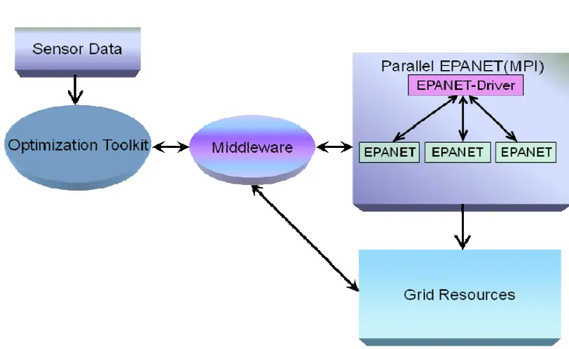
Fig 1.1 Basic Architecture of the Cyberinfrastructure
The above figure shows the high level architecture of the current cyberinfrastructure. The
optimization toolkit (which is a collection of optimization methods) interacts with the simulation
component (parallel EPANET) through the middleware. The middleware also communicates with the
grid resources for resource allocation and program execution. The various components of the
cyberinfrastructure are explained in detail in the following chapters. Simulation code enhancements
and middleware are discussed in the next chapter. Visualization, an important component of the
cyberinfrastructure is described in chapter 4 and conclusions and future work are presented in chapter
6
2
Problem Description and Optimization Methods
2.1
Contamination Source Characterization
Characterization of contaminant sources in a water distribution system (WDS) forms an integral part
of the overall threat management in urban WDSs. The source characterization problem involves
finding the contaminant source location and its temporal mass loading history (“release history”). The
release history includes start time of the contaminant release in the WDS, duration of release, and the
contaminant mass loading during this time.
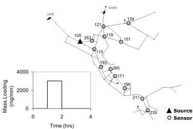
Fig 2.1. Water distribution network schematic and contaminant source mass loading profile. Node
numbers are labeled at the source and at the sensors.
For simplicity, we assume the existence of a single contamination source. This source is assumed to
be at one of the nodes in the water distribution system. With time, this contaminant spreads across the Sensor Source 105 263 121 129 151 119 115 193 265 171 199 211 239 0 2000 4000
0 2 4
7
system. Multiple source scenarios will be considered in future. The contaminant source is also
assumed be non reactive; i.e., it does not undergo any chemical reactions.
A few nodes are selected as the sensor locations in the water distribution system (See Fig 2.1). During
a contamination event, concentration readings are obtained at these locations at specified time
intervals. In the current scenario, the sensor locations are arbitrarily selected. Sophisticated algorithms
do exist for optimizing the placement of such sensors but that has not been the focus of this research.
A contamination source is assumed to be present at an arbitrary location in the water distribution
system for a predetermined period of time. Presently, we do not obtain the concentration
measurements from the real sensors on site. Instead a water quality simulation is run assuming the
existence of the contaminant at the specified location. The concentration readings which are obtained
from the simulation are then recorded for each sensor during every timestep. All these concentration
readings constitute a set of true source concentration profile readings.
To identify the true source, one starts out with a guess for the source location and its release history
i.e. start time of the contaminant, duration and the amount of contaminant present. For every such
guess, the water quality simulation is run to obtain the resulting concentration profiles for all the
sensor locations for every timestep.
The difference between the true source location readings and the guess source location readings is
then obtained. This amounts to one value for every sensor location for every timestep. The greatest
such difference is selected and the goal of the optimization method is to minimize the maximum error
value. The source characterization problem is thus posed as an inverse problem. The goal then is to
8
Mathematically, the source characterization problem can be expressed as
Find: NodeID, M(t), T0
Minimize Prediction Error ∑i,t || Cit(obs) – Cit(NodeID, M(t), T0) ||, where
• NodeID – contamination source location
• M(t) – contaminant mass loading(quantity) history at time t
• T0 – contamination start time
• Cit(obs) – observed concentration at sensors (readings for the guess source)
• Cit(NodeID, M(t), T0) – concentration from system simulation model (readings for the true
source)
• i – observation (sensor) location
• t – time of observation
2.2
Optimization Methods
This section describes the various optimization methods that were developed as part of this research.
2.2.1 Classical Random Search (CRS)
For solving a contamination source characterization problem, the goal is to find a source that
generates concentration profiles similar to those from the true source. A brute force approach to solve
this problem is to randomly generate a large number of source configurations (location and release
profile) and pick the one leads to concentration profiles that closely matches the observed values. We
term this approach “classical random search”.
For every trial (guess source), a number of parameters need to be generated (like the source location,
start time of contamination, duration of contaminant release, and the amount of contaminant release at
9
parameters have predetermined bounds. Hence random numbers need to be generated within the
respective bounds for each parameter for every trial.
After generating the parameters, the water quality simulation is run and the concentration profiles at
various sensor locations are obtained. If the difference between these readings and those of the true
source is below a certain threshold, the contamination source is correctly identified. Otherwise, a new
set of parameters (for next guess source) are generated and the process is repeated. The terminating
condition for the search could be a fixed number of trials or until a certain error threshold is reached.
2.2.2 Parallel Implementation
The Conventional Random Search (CRS) was initially a serial implementation and the limitations of
using a single processor were evident straightaway. The serial version was not able to handle a large
number of trials within a reasonable amount of time. Hence a parallel version of the CRS was
developed.
The total number of trials is divided equally among the available processors. If the number of trials is
not exactly divisible among the available processors, then the remaining trials are allocated to the
processors in order. The parallelization is implemented using MPI [9]. In a typical MPI program,
every processor hosts one process of the parallel program. Each process generates a different set of
random numbers to evaluate its allocated number of trials (guess sources). Every process uses a
different seed for initializing the random number generator and hence they are able to generate
different sets of random numbers. After computing all the trials, each process sends the results to the
master process. The master process aggregates all the results, computes the best result from them and
10
2.3
Evolution Strategies
Evolutionary algorithms (EA) are investigated as a search technique for solving the source
characterization problem by other members within the research group [10]. Beginning with a random
set of solutions, EAs evolve the population to iteratively converge to higher quality solutions. These
methods are flexible and can easily incorporate a simulation model into the search. Through the use
of a population of solutions, these algorithms explore the decision space independent of local gradient
information.
The EA investigated for solution of the source characterization problem is evolution
strategies (ES). As an archetypical EA, ES uses a population of solutions, or individuals, to search.
Each individual is comprised of a set of genes that, once decoded, represent the decision variables
that compose a solution to the problem. The performance of each individual to solve the problem is
represented by the fitness value; for the source characterization problem, fitness is the ability of an
individual to match closely chemical observations at sensor nodes. A fit solution is indicated by a
small value for the fitness, or prediction error. ES uses a set of search operators, including those that
create new individuals from old individuals and those that select high quality individuals to survive
11
3
Simulation Model Enhancements
3.1
Simulation Engine Overview
EPANET [11] is an extended period hydraulic and water-quality simulation toolkit developed at EPA.
It is originally developed for the Windows platform and provides a C language library with a well
defined API [12].
3.2
Wrapper
The original EPANET that was developed at EPA was customized to solve the source
characterization problem by developing a wrapper around the original version. The wrapper was
developed with the following design goals in mind.
3.2.1 Design Goals
Prior to the development of the wrapper, several optimization methods [10][13] were already created
for use in the project using diverse development platforms like Java and MATLAB respectively.
Hence the primary design goal was to interoperate with existing optimization methods.
The above mentioned optimization methods are based on evolutionary computation techniques. Every
stage of a typical evolutionary algorithm requires evaluation of a large number of simulations using
different contamination source parameters. Invoking a separate instance of the program for every
evaluation will be costly and unnecessary. Moreover there are aspects of the simulation which remain
unchanged between successive evaluations (e.g., hydraulic component of the simulation need not be
rerun between evaluations)
Thus the second design goal for the wrapper is to aggregate computation by evaluating multiple
12
sources within a single run. This will amortize the startup costs as well as eliminate redundant
computation.
3.2.2 Implementation
The wrapper was designed to receive different contamination source parameters from an input file.
The input file is chosen to be a normal text file in order to facilitate smooth interaction between the
wrapper and existing optimization methods.
During a single instantiation, the wrapper can successively perform EPANET simulations for each
trial contaminant source location. It evaluates the components of the simulation that are common to
all evaluations only once (e.g., reading the main input file, hydraulic part of the simulation if demands
do not change for different evaluations) and evaluates the varying portion of the simulation for the
different source locations (e.g., water quality component) thus saving considerable time. The results
are then written to an output file which can be fed back into the optimization method. The output file
is also a plain text file.
3.2.2.1 Input and Output
The input file contains the global simulation parameters including:
• EPANET input and output file names
• Total simulation time
• Number of timesteps
• Number of release timesteps (used to determine the duration of the contamination)
• Number of sensors and their location
13
The remainder of the input file contains the parameters for one contamination source per line. The
parameters for each source include the location, start time of the contaminant release and the amount
of contaminant during each of the release timesteps (known as release history).
The output file contains the prediction error value for each contaminant source location in the input
file.
3.3
Parallelization
The initial version of wrapper is a serial program. To effectively deal with problems of large size and
improve turnaround time, the wrapper had to be parallelized.
An individual EPANET evaluation can take anywhere from milliseconds to minutes depending on the
size of the WDS network, the number of time steps involved, and processor speed. Furthermore, the
problems that are currently being studied fall into the lower end of this spectrum. Therefore, the
computational burden arises from the large number of evaluations rather than each individual
evaluation. Hence there is no pressing need for performing fine grain parallelization where each
individual evaluation is parallelized.
3.3.1 Parallel Implementation
The parallel version of the wrapper is developed using MPI [8] and referred to as 'pepanet'. The following figure shows the details of the parallel implementation. Within the MPI program, the
master process reads the input file and populates data structures for storing global simulation
14
Fig 3.1. Detailed design of the parallel wrapper
The total contamination sources are then divided among all the processes. Each process then
simulates the assigned group of contamination sources successively. The root process collects results
from all the member processes and writes it to an output file. The workflow involved in computing
15
Fig 3.2 Detailed workflow within individual simulation
The parallel version of the wrapper (‘pepanet’) conforms to the same interface as the original
wrapper. Hence the changes made for parallelization are transparent to the optimization methods. If
needed, a serial version of the wrapper can still be obtained by compiling ‘pepanet’ using a
preprocessor switch
3.4
Motivation for Middleware Development
This section describes the motivation behind the development of the Cyberinfrastructure and its
components. The simulation code has evolved from a single simulation serial program (EPANET) to
16
The requisite computational resources may not be available on a single cluster. If the required
resources can be acquired at multiple sites, the parallel version can make use of grid enabled MPI
using Globus [7] Toolkit services (MPICH-G2) [14]. Still there is a performance penalty whenever
there is communication between the processes on different sites. Moreover every time the simulation
program needs to be invoked, one needs to submit the job to a batch scheduling system. This usually
results in a long wait time in the queue before the program is started.
Considering our scenario, the optimization method needs to invoke the simulation program at every
generation. If the simulation code experiences significant delays in the queue every time it starts up,
the total application will be a substantial amount of time waiting for the resources in the queue thus
increasing the overall wall clock time. Wall clock time is defined as the amount of time it took from
start to finish of the simulation-optimization package.
3.5
Persistent Wrapper
The evolutionary computing based optimization methods that are currently in use within the project
exhibit the following behavior. The method submits some evaluations to be computed, waits for the
results and then generates the next set of evaluations that need to be computed. There is unnecessary
cost associated with invoking the wrapper separately for every generation.
In addition to amortizing the startup costs, the wrapper significantly reduces that wait time in the
queue in a job scheduling system. As explained in section 4.1 above, if the simulation code were to be
separately invoked every generation, the simulation program needs to wait in a queue for acquiring
the requisite resources. But if the wrapper is made persistent, the program needs to wait in the queue
just once when it is first started. Hence the wrapper (‘pepanet’) has been modified to create a version
17 3.5.1 File based Communication
The persistent wrapper achieves this by taking out some of the common computation from
evaluations submitted to it across generations. It then loops around waiting for a sequence of input
files whose filenames follow a pattern. This pattern for the input and output file names can be
specified as command line arguments facilitating flexibility in placement of the files as well as
standardization of the directory structure.
The current version of the persistent wrapper is still generic enough and does include certain amount
of redundant computation across generations. This is by design since the wrapper has been initially
designed to be stateless across generations. If needed, the persistent wrapper could be optimized to
run a particular problem scenario by eliminating redundant computation that is presently involved.
3.6
Middleware
Consider the scenario when the optimization toolkit is running on a client workstation and the
simulation code (‘pepanet’) is running at a remote supercomputing center. Communication between
the optimization and simulation programs is difficult due to the security restrictions placed at today’s
supercomputing centers. The compute nodes on the supercomputers cannot be directly reached from
the external network.
In light of these obstacles, a middleware framework has been developed to facilitate the interaction
between the optimization and simulation components. The middleware component utilizes public key
cryptography to authenticate to the remote supercomputing center from the client site. The
middleware then transfers the input file from the optimization component to the simulation
component on the remote site. It then waits for the computation to be finished and then fetches the
output file back to the client site. This process is repeated till the solution is reached. The basic
18
Fig 3.3 Basic functionality of the Middleware
3.7
Teragrid deployment
In this scenario, the optimization toolkit (JEC) is executed on Neptune, the local cluster at NCSU.
The simulation component (persistent ‘pepanet’) is executed on a remote supercomputer, in this case,
the Teragrid Itanium cluster at NCSA (Mercury).
3.7.1 Workflow
A public and private key combination is generated on Neptune. The public key is then copied over to
the NCSA cluster and added to the list of authorized keys to be permitted access. The private key is
present on Neptune and is used by ‘ssh-agent’ to authenticate to the NCSA cluster automatically
whenever authorization is requested.
Now, the file transfer between the client site (Neptune) and remote site (Mercury) is entirely
transparent to the optimization toolkit on the local site.
3.8
SURAgrid deployment
The Southeastern Universities Research Association (SURA) is a consortium of over sixty
universities across the US. SURAgrid is a consortium of organizations collaborating and combining
19
deployment scenario, the optimization toolkit (JEC) is executed on Neptune, the local cluster at
NCSU. The simulation component (persistent ‘pepanet’) is executed on a remote SURAgrid resource.
3.8.1 Grid Workflow
To be able to run jobs on SURAgrid, the NCSU user applies for an affiliate user certificate issued by
SURAgrid site Georgia State University (GSU), who has a Certificate Authority (CA) that has been
cross-certified with the SURAgrid Bridge CA (BCA). Cross-certification enables SURAgrid resource
sites to trust the user certificate being presented by the NCSU user and when the SURAgrid User
Administrator at GSU also creates a SURAgrid account for the NCSU user, the user essentially has
single-sign-on access to SURAgrid resources at cross-certified SURAgrid sites1. After they’ve
authenticated to the SURAgrid resource, the user add the user’s public key on Neptune to the
authorized keys list on the SURAgrid resource. The user then invokes the optimization method on
the client workstation which initiates the middleware. The middleware directly communicates with
the specific SURAgrid resource (authenticated through ssh keys) for job submission and intermediate
file movement. Currently the application needs to be pre-staged by the user but this functionality will
be integrated into the middleware.
NCSU users running the integrated simulation-optimization system software will use its
“middleware” feature, which uses public key cryptography to provide a seamless, python-based
application interface for staging initial data and executables, data movement, job submission, and
real-time visualization of application progress. The interface uses commands over ssh to create the
directory structure necessary to run the jobs and handles all data movement required by the
application. It launches the jobs at each site in a seamless manner, through their respective batch
commands. The middleware is able to minimize resource queue time by querying the resource at a
1NCSU users may also need to obtain a local account from cross-certified resource sites that have additional authorization
20
given site to determine the size of resource to request. Most of the middleware functionality has been
implemented at least at a rudimentary level and efforts are now focused on enhancing integration and
sophistication.
3.9
Advanced functionality
The ultimate goal of this research is to produce a cyberinfrastructure that will be able to harness
multiple grid resources in order to perform real-time, on-demand computing to solve water
distribution threat management problems. This infrastructure will integrate various components such
that the measurement system, the analytical modules and the computing resources can mutually adapt
and steer each other. In the future, the team plans to improve application’s functionality in grid
environments by focusing on the dynamic aspects of resource demand, availability, and allocation.
To utilize multiple grid resources, one has to be able to divide the required computation task among
the available grid resources. For instance, consider the scenario where you need to evaluate 10k
simulations using 64 processors and the available grid resources are 48 processors at one site and 16
processors at the other site. Then the task is distributed by allocating 7500 simulations to be
performed at the first site and the remaining 2500 are performed at the second site. This method could
be applied to divide any computation task among multiple grid resources.
3.9.1 Helper programs
For the above method to work, one needs to have access to helper program to split a simulation input
file into the requisite number of parts containing the specified number of simulation parameters. Such
a helper program has been developed. In the above example, the program can take the original input
file and split it to produce two input files containing 7500 and 2500 simulation parameters
21
Likewise, there should be another helper program that could take the output files produced from
evaluating fragmented input files like those in our example and merge them to form a single output
file in the correct order. Such a program is needed to ensure transparency of the fragmentation
process from the perspective of the optimization method. This program has also been developed and
successfully demonstrated.
3.9.2 Intelligent Resource Requisition
Whenever a program is submitted to a job scheduling system, the resource requisition can be made in
such a way as to reduce the wait time in the queue. This may improve the turnaround time of the job
in some cases but is not assured. But if the job requirement is to make progress as soon as possible
then the following strategy could be used. This could be achieved by requesting the amount of
resources equivalent to those that will become available at the earliest. This is achieved on a PBS
(Maui/Moab) job scheduling system using the ‘showbf’ command. This command provides
information regarding the backfill window in the scheduling system as well as information regarding
the earliest availability of resources. But unfortunately this does not guarantee the availability of such
resources at the predicted time.
Recent interaction with the staff at Cluster Resources Inc. shed some light on other facilities in the
scheduling system that give a better prediction of the resource availability and provide a programmer
friendly interface. These include features that allow the collection of statistics regarding job
submission and resource availability. Then the expected start time of a program can be calculated
based on historic data or the current reservation data. The middleware will include this functionality
22
3.10
Performance
3.10.1 Test Platforms
Neptune is a 11 node Opteron Cluster at NCSU. It has 22 2.2 GHz AMD Opteron(248) processors
and a GigE Interconnect.
The Teragrid Linux Cluster at NCSA has 887 IBM nodes of which 256 nodes have dual 1.3 GHz Intel
Itanium 2 processors and 631 nodes have dual 1.5 GHz Intel Itanium 2 processors and are connected
using a Myrinet interconnect
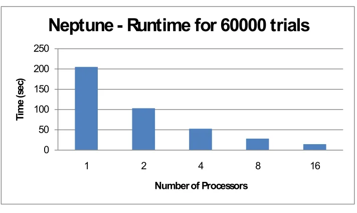
3.10.2 Wrapper Performance
The following figures show the performance of the wrapper for different simulation sizes. In each
case, the input file has been pre-generated. It can be noticed that the wrapper scales well with the
increase in number of processors as well as with simulation size.
0 0.5 1 1.5 2 2.5
1 2 4 8 16
Ti
m
e (
se
c)
Number of Processors
Neptune - Runtime for 600 trials
23 0 5 10 15 20 25
1 2 4 8 16
Ti
m
e (
se
c)
Number of Processors
Neptune - Runtime for 6000 trials
Fig 3.5. Runtime for 6000 Trials, by Number of Processors on Neptune
0 50 100 150 200 250
1 2 4 8 16
Ti
m
e (
se
c)
Number of Processors
Neptune - Runtime for 60000 trials
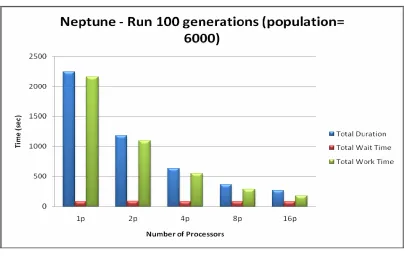
24 3.10.3 Application Performance on Neptune
The following figures show the performance of simulation and optimization components working in
conjunction through middleware for various problem sizes. It can be noticed that the entire
application scales well with the increase in number of processors as well as with simulation size.
0 50 100 150 200 250
1p 2p 4p 8p 16p
Ti
m
e (
se
c)
Number of Processors
Neptune - Run 100 generations
(population= 600)
Total Duration
Total Wait Time
Total Work Time
JEC runtime - 8.6 - 10.2 sec
25
Fig 3.8. Runtime for 100 Generations (Population 6000), by Number of Processors on Neptune
Preliminary performance analysis revealed that the total waiting time within the simulation code
increased when the optimization toolkit and root process of the wrapper are on different nodes on the
cluster. When both of them are placed on the same compute node, wait time reduced substantially. At
this stage, it had been identified that the sleep timer resolution served as the lower bound for the
application’s wait time. Hence the timer resolution has been tuned both within the wrapper and the
middleware to achieve tradeoff between polling interval and reducing wait time. The results of these
26 0 500 1000 1500 2000 2500 3000 3500
16p - JEC,Root process(Wrapper)
- Different nodes
16p - JEC,Root process (Wrapper)- same
node
16p - JEC,Root process(Wrapper) - same node,optimal sleep timers Ti m e( se c)
Neptune – Improvements
Total Duration
Total Wait Time
Total Work Time
Fig 3.9 Performance improvements on Neptune
3.10.4 Application Performance on Teragrid
In this case, the optimization toolkit resided on the local cluster Neptune and the simulation
component was executed on NCSA Teragrid cluster. The following figures show the performance of
simulation and optimization components working in conjunction through middleware for various
problem sizes. Compared to the earlier scenario on Neptune, it can be noticed that the wait time has
increased substantially due to the communication overhead involved in transferring files from local
cluster to Teragrid cluster. The wait time distribution is shown in the following table.
Table 3.1 Wait time distribution (Total generations -100)
Simulation size per gen
Total JEC time(s)
Input size Total Input copy time(s)
Output size Total Output copy time(s)
600 trials 13-14 200 KB 240-250 5.3 KB 50-60
27 0 200 400 600 800 1000 1200
1p 2p 4p 8p 16p
Ti
m
e (
se
c)
Number of Processors
Teragrid - Run 100 generations
(population=600)
Total Duration Total Wait Time Total Work Time
Fig 3.10 Runtime for 100 Generations (Population 600), by Number of Processors on Teragrid
0 500 1000 1500 2000 2500 3000
4p 8p 16p
Ti
m
e (
se
c)
Number of Processors
Teragrid - Run 100 generations
(population=6000)
Total Duration Total Wait Time Total Work Time
28
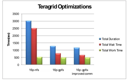
Performance analysis of the application revealed that the file system used to execute the simulation
had a significant impact on the wait time. The performance improved when the application is moved
from a NFS file system to a faster GPFS file system. Further improvement in wait time has been
achieved by consolidating the network communications within the middleware. The following figure
shows the performance gains achieved in each case.
0 500 1000 1500 2000 2500 3000 3500
16p-nfs 16p-gpfs 16p
-gpfs-improved comm
Ti
m
es(
se
c)
Teragrid Optimizations
Total Duration
Total Wait Time
Total Work Time
Fig 3.12 Performance improvements obtained using better file system and consolidating middleware
communications on Teragrid
The following figures show the performance improvements obtained by consolidating middleware
29 0 100 200 300 400 500 600 700 Ti m e ( se c)
Number of Processors
Teragrid - (Improved)Run 100 generations
(population=600)
Total Duration
Total Wait Time
Total Work Time
Fig 3.13 Performance improvements obtained by consolidating middleware communications for
population size of 600 per generation for 100 generations
0 200 400 600 800 1000 1200 1400
16p 16p-imp 32p-imp
Ti
m
e (
se
c)
Teragrid - (Improved) Run 100
generations (population=6000)
Total Duration Total Wait Time Total Work Time
Fig 3.14 Performance improvements obtained by consolidating middleware communications for
30
The following figures show the read/write performance for the different simulation sizes on Teragrid.
The read/write times remain constant even as the number of processors increased since only the root
process performs the input/output.
0 0.2 0.4 0.6 0.8 1
1p 2p 4p 8p 16p
Ti
m
e (
se
c)
Number of Processors
Teragrid - 100g-600pop Read/ Write
Total Read Time Total Write Time
Fig 3.15. Teragrid Read/Write Time for 100 Generations (Population 600)
0 0.5 1 1.5 2 2.5 3 3.5 4
4p 8p 16p
Ti
m
e (
se
c)
Number of Processors
Teragrid - 100g-6000pop Read/ Write
Total Read Time Total Write Time
Fig 3.16. Teragrid Read/Write Time for 100 Generations (Population 6000
31 0 0.01 0.02 0.03 0.04 0.05 0.06 0.07 0.08
1p 2p 4p 8p 16p
Ti
m
e (
se
c)
Number of Processors
Neptune- 100g-600pop Read/ Write
Total Read Time Total Write Time
Fig 3.17. Teragrid Read/Write time for 100 Generations (Population 600)
0 0.1 0.2 0.3 0.4 0.5
1p 2p 4p 8p 16p
Ti
m
e (
se
c)
Number of Processors
Neptune- 100g-6000pop Read/ Write
Total Read Time Total Write Time
32
4
Visualization
4.1
Motivation
During the course of this research, we identified the need for a visualization tool as it was
cumbersome and practically impossible to sift through the final and intermediate output of the
optimization methods and understand the search patterns, efficiency and convergence of the methods.
Eventually, the visualization tool became an important component of the cyberinfrastructure
providing support for real time visualization for monitoring application’s progress.
The visualization tool has been developed using Python [15], Tkinter [16][17] and Gnuplot [18]. The
tool was developed keeping the following goals in mind.
1. Visualize the water distribution system and help understand the locations where the
optimization method is currently searching
2. Visualize how the search is progressing from one generation to the next
3. Facilitate understanding of the convergence pattern of the optimization method
The tool provides the following functionality.
1. Visualizes the water distribution network
2. Displays the true location of the contamination source
3. Displays the source locations where the optimization algorithm is currently searching
4. Displays the best estimate for the location of the contamination source
33
6. Displays the concentration profile of the best estimate of the contamination source
4.2
Representation
A water distribution system is modeled as a graph where the edges represent the pipes connecting the
nodes and nodes represent a junction of pipes or a water source (like a tank or a lake).
The concentration profile of a contamination source is depicted in a graph plotting the mass loading
(quantity) of the contaminant versus the timestep.
4.3
Node mapping
For simulation of a water distribution system (WDS) using EPANET, the information for the WDS is
provided in a specific input format. The input file contains vital information that is used for
visualizing the WDS.
The information includes details of the node connections and coordinates for the locations of the
various nodes. But the optimization methods use a different numbering for the nodes instead of the
numbering used in the input file. The numbering scheme used by the optimization methods is actually
equivalent to an internal numbering scheme within the EPANET simulation program. So, a helper
program has been written to perform this mapping between the different numbering schemes.
To perform the mapping, the program utilizes the EPANET toolkit functionality to obtain the
information regarding the internal numbering scheme. It also captures the information for every pipe
that provides information regarding the connections among the nodes. All this information is then
written to an output file which is used by the visualization tool. The output file also contains a section
34
4.4
Initial design
The visualization tool reads in an input file containing the WDS information as well as the output
from the node mapping helper program described above. It generates the WDS map. The tool also
needs information about the optimization method search pattern.
Please recall that the optimization method generates an input file every generation for use by the
simulation code (‘pepanet’ in our case) and the results from the simulation code are written to an
output file. This output file is then used by the optimization method to generate the next input file for
the next set of evaluations.
So, the visualization tool needs to access the above two files for every generation before updating the
WDS map with the search pattern information.
The initial design for the visualization tool had a single thread of control handling both I/O and
visualization aspects. So the tool rendered the WDS map and then would wait for the input and output
files from the optimization method. After it receives both files, the tool updates the WDS map
showing the locations where the method is currently searching. It also displays the best estimate of
35
Fig 4.1. Initial Visualization Tool Rendering
4.4.1.1 Limitations
The initial design of the tool paved way for certain usability issues. Since the tool had a single thread
of control, the user will not be able to interact with the graphical interface of the tool while it is
waiting for the files. The tool would not respond to the user input during this wait period.
The initial version of the tool needed manual input (clicking ‘Next Generation’ button shown above)
from the user to proceed to the next generation. Hence this is not amenable to real time visualization
36
4.5
Final design
The final version of the visualization tool includes a major redesign of the backend as well as
enhanced functionality. Some of the salient enhancements are:
• Multithreaded design that eliminated the usability problems
• Provided automatic updating of the map whenever new data (next generation) is available.
• Included ‘pause’ and ‘resume’ functionality for the automatic updating enabling an user to
use the visualization tool at his own pace
• Displays concentration profiles of the true and estimated sources
• Generates and archives the images of the WDS map and the concentration profiles for every
generation.
37
Fig 4.2 Improved Visualization Tool User Interface
4.5.1.1 Multithreading
To overcome the limitations of the initial design, the visualization tool has been rewritten using a
38
interface and the other thread taking care of the I/O. So the user can interact with the tool while the
background thread is waiting for the files to update the display.
Whenever the files become available, the background thread reads the files, parses them and extracts
the requisite information like the source locations currently searched. It also calculates the best
solution among all the trials within that generation. It then puts all this information onto a queue data
structure for consumption by the other thread.
The thread handling the GUI periodically checks the queue for any data. Whenever it finds any data,
it dequeues the data and updates the WDS map with the information.
4.5.2 Source Location
39
This section describes the interface elements representing the source locations on the WDS map. All
nodes in the WDS are marked by a ‘white’ circle by default. The source locations that are currently
being searched are indicated by a ‘cyan’ colored circle. The true contaminant source location is
indicated by a ‘red’ circle. The best estimate of the contaminant location is indicated by a relatively
large ‘green’ circle.
4.5.3 Concentration profile
Fig 4.4. Concentration Profile Shown by the Visualization Tool
The concentration profile of the contaminant source is plotted using Gnuplot. The graph plots the
contaminant mass loading (quality) against the release timesteps. The graph depicts two concentration
40
4.6
Visualizing Optimization method progress
The following screenshots illustrate the important stages of the optimization method’s search process.
During the initial generations of the optimization algorithm, the estimated solution and concentration
profile do not coincide with those of the true source.
41
Fig 4.6.Concentration Profile – Generation 0
After several generations, the optimization method is able to identify the contaminant source location.
Hence the true and estimated source locations coincide.
42
Still, the concentration profiles of the true and estimated sources may not match completely.
Fig 4.8. Concentration Profile – Generation 47
After further searching, the optimization method is able to more accurately identify the concentration
43
Fig 4.9. Source Location – Generation 65
44
4.7
Performance
The visualization tool has been successfully tested and is capable of visualizing large water
distribution systems. The larger WDS that we used for scalability testing consists of 12,527 nodes and
14,831 links and is shown below.
Fig 4.11. The Large Water Distribution System
The smaller network has 97 nodes and 119 links. The large WDS has 12,527 nodes and 14,831 links.
The following table shows the file read time and map rendering time for both water distribution
45
Table 4.1 Read Time and Rendering times for different water distribution networks
Water Distribution Network
Map File Read Time (sec) Map Rendering Time (sec)
Small network 0.0083 0.1970
46
5
Conclusions and Future work
To address the need for solving the contamination source characterization problem in water
distribution systems, an end to end solution was developed. The framework was successfully
deployed in a grid environment, and the application demonstrated that the overall turnaround time has
been minimized. The visualization tool developed as part of this research facilitated real-time
monitoring of the application’s progress.
An illustrative water distribution network was used to demonstrate the framework. The simulation of
this small system represents a worst case scenario, as the computation to communication time ratio is
relatively small. In the future, the framework will be applied for large water distribution systems,
involving longer simulation times and more computation within a single EPANET evaluation (by
recalculating hydraulics more frequently). As the input and output files will remain the same size, the
communication time will remain unchanged, while the computation time increases significantly.
Hence the wait time of the application will be considerably lower than the computation time thereby
improving the utilization of the computational resources.
The significant communication times incurred while deploying the framework on Teragrid cluster
emphasize the need for using low latency, high bandwidth backbone networks for communication.
Moving forward, specialized file transfer clients [19] using GridFTP [19], a high-performance,
secure, reliable data transfer protocol optimized for high-bandwidth, wide-area networks must be
utilized to leverage the benefits of such backbone networks. Additionally, the middleware
functionality demonstrated in this research will be integrated into existing workflow systems like
Kepler [8] and CogKit [6] to provide a improved feature set for the benefit of the end user, the
47
The inherent design of the current optimization methods requires synchronization at every generation
inducing a delay before generating parameters for the next set of evaluations thereby restricting the
amount of computation that could be performed per generation. Hence the need for asynchronous
optimization methods has been identified and future work will focus on development of such
48
6
References
1. G. Mahinthakumar, G. von Laszewski, S. Ranjithan, E. D. Brill, J. Uber, K. W. Harrison, S.
Sreepathi, and E. M. Zechman, An Adaptive Cyberinfrastructure for Threat Management in
Urban Water Distribution Systems, Lecture Notes in Computer Science, Springer-Verlag, pp.
401-408, 2006.( International Conference on Computational Science (3) 2006: 401-408)
2. Darema, F. Dynamic data driven applications systems: New capabilities for application
simulations and measurements. Lecture Notes in Computer Science 3515, pages 610–615, 2005.
3. Daniel E.Atkins et al, Report of the National Science Foundation Blue-Ribbon Advisory Panel
on Cyberinfrastructure January 2003 http://www.communitytechnology.org/nsf_ci_report/
4. Water Science and Technology Board, A Review of the EPA Water Security Research and
Technical Support Action Plan: Parts I and II, The National Academies Press, 2003.
5. von Laszewski, G. and Hategan, M. Java CoG Kit Workflow Concepts, in Journal of Grid
Computing, Jan. 2006. http://www.mcs.anl.gov/~gregor/papers/vonLaszewski-workflow-jgc.pdf.
6. von Laszewski,G., Jarek Gawor, Peter Lane, Nell Rehn, Mike Russell, and Keith Jackson ,
Features of the Java Commodity Grid Kit. in Concurrency and Computation: Practice and
Experience
,14:1045-1055,2002.http://www.mcs.anl.gov/~gregor/papers/vonLaszewski--cog-features.pdf.
7. The Globus Project. Web Page. Available from: http://www.globus.org.
8. Kepler: An Extensible System for Design and Execution of Scientific Workflows, I. Altintas, C.
Berkley, E. Jaeger, M. Jones, B. Ludäscher, S. Mock, system demonstration, 16th Intl. Conf. on
Scientific and Statistical Database Management (SSDBM'04), 21-23 June 2004, Santorini Island,
Greece.
9. The Message Passing Interface (MPI) standard Web Page http://www-unix.mcs.anl.gov/mpi/
49
in Engineering Design, submitted to: Genetic and Evolutionary Computation Conference
(GECCO) 2006, ACM.
11. Rossman, L.A.., EPANET Users Manual. Risk Reduction Engrg. Lab., U.S. Evnir. Protection
Agency, Cincinnati, Ohio, 1994.
12. Rossman, L.A.. The EPANET programmer’s toolkit. In Proceedings of Water Resources
Planning and Management Division Annual Specialty Conference, ASCE, Tempe, AZ, 1999.
13. Liu, L. and S. R. Ranjithan, Adaptive Niched Co-Evolutionary Algorithm (ANCEA) for
Dynamic Optimization, submitted to: Genetic and Evolutionary Computation Conference
(GECCO) 2006, ACM.
14. MPICH-G2 Project. Web Page. http://www3.niu.edu/mpi/
15. The Python programming language. Web Page. http://www.python.org/
16. Tkinter: GUI Programming toolkit for Python. http://wiki.python.org/moin/TkInter
17. Fredrik Lundh, An Introduction to Tkinter, Available online at
http://www.pythonware.com/library/tkinter/
18. Gnuplot Project. Web Page. http://www.gnuplot.info/
19. GridFTP Usage on Teragrid. Web Page. http://www.teragrid.org/userinfo/data/gridftp.php