CHILD BENEFITS AND WELFARE FOR CURRENT AND FUTURE
GENERATIONS:
SIMULATION
ANALYSES
IN
AN
OVERLAPPING-GENERATIONS MODEL WITH ENDOGENOUS FERTILITY
Kazumasa Oguro
Associate Professor, Institute of Economic Research Hitotsubashi University, Japan
Manabu Shimasawa
Senior Researcher, National Institute for Research Advancement, Japan
Junichiro Takahata
Assistant Professor, Dokkyo University, Japan
ABSTRACT
We constructed an overlapping-generations model with endogenous fertility to analyze the effects of child benefits and pensions on the welfare of current and future generations. The following results were obtained. First, in the case without pension and accelerated fiscal reforms, the best policy to improve the welfare of future generations is to finance the provision of child benefits by capital taxation, followed by issuing government debt, consumption taxation (VAT), and wage taxation, in that order. Second, debt reduction coupled with increasing child benefits is preferable to debt reduction alone to reduce public debt for future generations. In particular, coupling increased child benefits and fiscal reform simultaneously stands out as the most desirable option. Third, from the viewpoint of pension reform, maintaining pension benefits by increasing VAT is better than cutting benefits coupled with increasing child benefits for future generations.
Keywords:
Overlapping-generations model; child benefit; endogenous fertility; theorem of zero capital taxAsian Economic and Financial Review
INTRODUCTION
This paper aims to analyze the effect of child benefits and pensions on the welfare of current and future generations, by constructing an overlapping-generations (OLG) model with endogenous fertility1.
The decline in fertility rate is a major concern for the Japanese economy. The reason for this is that an economy with a low birth rate and an aging population has created serious problems in terms of the sustainability of fiscal and social security systems, including public pension. In order to maintain sustainability, we have several policy choices. The first is to promote fiscal reform, e.g., increase consumption tax. The second is to carry out social security reform, e.g., decrease public pension benefits. The third is to revise the population trends, e.g., increase fertility rate by expanding child benefits. The Japanese government has attempted to work with the first and the second policies. However, due to conflicting interests between younger and older generations, obtaining an agreement on the reform by both generations is often too difficult for the government to achieve. Therefore, the government is trying to promote child benefits expansion as the third policy. Consequently, we should consider how to finance child benefits expansion. In general, the financial resource selection to provide child benefits determines the type of welfare effects on current and future generations. At this point, key research results on the OLG models with exogenous versus endogenous fertility should be compared.
For the standard OLG model represented by Diamond (1965) and others, it is well established that consumption taxation (VAT) is the most effective method to raise financial resources for the welfare of future generations, followed by wage taxation and capital taxation, the second and third methods of choice, respectively, given the future path of government expenditure. This can be explained as follows. The first benchmark is the theorem of zero taxation of capital income, derived from (Atkinson and Stiglitz, 1972) the orem of optimal tax. The theorem is best understood by considering the OLG model with two generations, working and retired, living concurrently. At the first period (working period), each generation earns wage income by providing labor force, consumes a part of that income, and saves the remainder. At the second period (retired period), the retired generation consumes the principal and the interest derived from that saving. In this setting, Atkinson and Stiglitz (1976) have proved that the case in which the consumption tax of the first
period is different from that of the second period is not optimal. In addition, since these respective differing consumption taxes have the taxation property for the interest on the savings consumed in
1
In our paper, child benefits cover the total cost of child rearing and child care, but we do not distinguish between benefits
in cash (e.g., child benefit) and benefits in kind (e.g., subsidies for using nursery and forreceiving high education).
the retired period, this theorem suggests that zero taxation of capital income is optimal; it holds in the OLG model with multi-concurrent generations and exogenous fertility2. Similarly, Chamley (1986) and Judd (1985) also indicate that zero taxation of capital income in the OLG model with
exogenous fertility and taking over inheritance among generations is most effective in the long term. Moreover, on the steady state, the equation (1 – wage tax rate) × (1 + consumption tax rate) = 1 holds and consumption taxation becomes equivalent to wage taxation with no borrowing constraint and no change in government policies. Because of this, a switch in government policies from wage-based to consumption-based taxation, if implemented at a tax rate equivalent to that described previously, may have no influence on the generation immediately after the policy change, but the effect during the transition period may differ. Taxation on the retired generation’s consumption in the early stage of the transition period presents less distortion as it works like a lump-sum tax. In other words, considering intertemporal government budget constraints with the zero-sum feature of intergenerational income transfer, this policy would result in a transfer of income from the retired generation to the working and future generations. An increase in the public debt tends to instigate the crowding-out effect, which may lead to a restrained accumulation of capital and a decrease in future economic growth. In the same manner, according to Hatta and Oguchi (1999), among others, the pay-as-you-go public pension also carries an ―implicit debt‖ of
approximately 150% of GDP and may inhibit future growth. Although public pensions transfer income from the working and future generations to the retired generation, implementation of the above-mentioned policies would have the opposite effect, transferring the income from the retired generation to the working and future generations, resulting in an increase in capital accumulation and enhanced future growth. From this we can infer that, in the standard OLG model with exogenous fertility and given the future path of government expenditure, consumption taxation (VAT) would most often be the optimal source of funding for expenditure, followed by wage taxation and capital income taxation, in that order. However, as the assumptions in the OLG model with exogenous fertility are realistically modified, the conclusions drawn—such as the theorem of zero taxation of capital income—begin to differ. For example, Cremer and Gahvari (1995) indicated that if the wage income in the second (retired) period is uncertain, it is desirable that the taxation imposed on the second-period consumption is higher than that of the first (working) period. This means that capital income taxation is desirable.
Similarly, Conesa et al. (2007) suggest that, when life expectancy and wage income are uncertain, a capital income tax is desirable. Saez (2002) adds that zero capital taxation is not always optimal, as the desirable savings rate differs with varying levels of individual skill. Moreover, Weinzierl
2
The reader should remember that Atkinson and Stiglitz’s (1976) partial equilibrium analysis greatly influences the optimal
tax rule,while considering the OLG model with exogenous fertility based on the evaluation criteria of the growth process
(2007) shows that, when wage income varies with age and there are heterogeneous demographics, a
15% tax would increase social welfare more than the zero-taxation scenario. In addition, Hubbard and Judd (1986) found that, when the capital market is incomplete and there are borrowing
constraints, the implementation of capital taxation can be justified. As described above, modifications by Atkinson and Stiglitz (1976) suggest that there are various justifications for the implementation of capital taxation. However, these are based on the OLG model with exogenous fertility; research on the justification of capital taxation, assuming the OLG model with endogenous fertility, remains insufficient. Our results show that the child-rearing cost is the key parameter in the OLG model with endogenous fertility. For example, zero capital taxation may no longer be considered optimal if the child-rearing cost is an increasing function of lifetime income. This can be explained as follows. First, zero capital taxation is desirable in the standard OLG model with exogenous fertility; however, in comparison to nonzero capital taxation, both lifetime income and child-rearing costs increase for future generations. If the positive effect of increased lifetime wages is overshadowed by a larger negative effect of increased child-rearing costs, the relative value of lifetime wages for child-rearing costs decreases due to the lifetime budget constraints of each generation. In such a case, although the implementation of capital income taxation is in fact justified, research based on the OLG model with endogenous fertility is not being pursued.
On the basis of the findings of Oguro et al. (2009), we construct an OLG model with multi-concurrent generations and endogenous fertility, assuming consumption, wage, capital, and other taxations as potential funding sources for increased child benefits, to analyze the effect on the welfare of each generation. We then analyze the effect on the welfare of each generation from the perspective of future social security reforms in two hypothetical cases: reducing pension benefits and using consumption tax to partially fund pension benefits. According to our simulation results, the welfare for the future generation in the case with child benefits expansion funded by capital income tax is greater than in the case with child benefits expansion funded by consumption tax. This indicates that zero taxation of capital income in the OLG model with endogenous fertility is not the most effective in the long term. Our research is organized as follows. In Section 2, we explain the OLG model with multi-concurrent generations and endogenous fertility used in this paper. In Section 3, we describe the data, as well as the calibration and simulation scenarios used in our research. In Section 4, we evaluate the simulation results. Finally, in Section 5, we summarize our results and suggest topics for future discussion.
The Model Structure
utility function with consumption and the number of children. The representative competitive firm has a standard Cobb–Douglas production technology and maximizes its profits. In our model, not only the goods market but also factor markets are perfectly competitive. The model has five main building blocks: (1) household behavior, (2) firm behavior, (3) the public pension, (4) the government, and (5) market equilibrium. Details of each block follow.
Household Behavior
There is a representative individual for each generation in the household sector. We assume that preference forms are the same for all agents in all generations. Moreover, each individual lives for a fixed number of periods. In each period of the model, the oldest generation dies and a new one enters. Further, the representative individuals maximize their intertemporal utility function with consumption and the number of children subject to their lifetime income. They are also assumed to be rational and with perfect foresight. Each generation enters the labor market at age 21, bears and brings up their children at ages 21 to
M
+ 20, retires at ageQ
1, is granted a pension atQ
, and dies at age Z. In addition, each supplies labor inelastically, and the utility functions of the t-th generation born in year t are specified as:2 1 , 20
1 1
1
1 1
1 )
1 ( 1
2 1
j t Z
j
j t
t
c n
U (1)
where refers to the weight between number of children and consumption, 1 the preference parameter of number of children, j the j-th period of life, the pure rate of time preference, and
2 the reverse of the elasticity of intertemporal substitution of consumption. The arguments of the
utility function are the number of children (nt) and the consumption per period (ct,j).
In addition, we assume that the number of children (nt,j) whom the t-th generation bears at the j-th
period of life is the following:
t j j t p n
n, (where pj 0 (if 1 j M 20) and pj 0 (if j M 20)), (2)
wherepj refers to the possibility that each generation bears the children at the j-th period of life
and this parameter is assumed to be exogenous.
Moreover, the technological progress is assumed to be exogenous and labor embodied. We model age-specific labor productivity by assuming a hump-shaped age-earnings profile, that is, a
quadratic form of its age j, so its age-wage profile
e
j takes the following form:2 2 1
0
j
j
e
j , 0, 1 0and 2 0 (3)t Z
j j
k tk
j t j t M
j g j g
k tk
j t g j t g j t NW RN c tc RN n
tc 2 0
1
1 2 0 , 2 0 2 0 1 2 0 1 1
1 2 0 , 2 0 1 2 0 ) 1 ( ) 1 ( ) 1 ( 2 0 2 0
1 2 0
2 0 2 0 2 1
1
1 2 0
2 0 2 0
2 0
2 0 ) (1 ) (1 )
1
( Z
Q
j j
k tk j t j t Q j j
k tk
j j t j t j t j t RN q p RN e w w tw ,(4)
where 1/ RN refers to the factor of the present discounted value derived from the gross interest
rate after tax RNt 1 (1 trt)rt, the rate of returnrt, and the capital tax trt in year t, and g is the
child-rearing cost at the g-th period of life; t is the government subsidy in year t; tct is the consumption tax rate in year t; twt is the labor income tax rate in year t; wtis the public pension premium rate in year t; NWtis the net lifetime income of generation t; wtis the wage rate in year t;
t
p is the tax for pension benefit in year t; and qt stands for the pension benefit in year t.3 In addition, the child-rearing cost is assumed to be proportional to net lifetime income; that is,
) 1
/( t
t g
g NW tc , where g is the constant parameter and tct the average rate of
consumption tax imposed on the t-th generation.
Each generation maximizes its utility function (1) under the budget constraint (4).
When , the maximization procedure differentiating the household utility function (2)
with respect to and , subject to the individual’s lifetime budget constraint (4), yields the
following equations concerning consumption per period and number of children.
/ 1
1 20 20
, (1 )
1 1 ) 1 ( j
k tk
j t j j t RN tc c , / 1 20 1 20 1 1 1 20 20 1 20 ) 1 ( ) 1 ( M
j g j g
k tk
j g j t g j t t RN p tc
n , (5)
and
t Z
j
j k tk
j t
j
M
j g j g
k tk
j g j t g j t NW RN tc RN p tc 2 0
1 1/ 1
1 2 0
2 0 / / 1 1 / 1 2 0 1 2 0 1 1
1 2 0
2 0 1 2 0 / 1 / 1 ) 1 ( 1 1 ) 1 ( ) 1 ( ) 1 (
3
In Japan, there are some indirect taxes (e.g., alcohol and tobacco tax) other than consumption tax. We calculatethe indirect
tax rate from the total amount of indirect tax revenue in the national account. The rate is about 12%. 5% is the consumption
tax rate and 7% the other indirect tax rate. Therefore, the effect of the other indirect tax rate is also considered in our
simulation. However, in the simulation, we focus on the effect of increased consumption tax. Hence, we let tct represent
the consumption tax only in our paper. 2
1
If the parameter is stable, these equations dictate the following two relationships: (1) as in any
life-cycle model, the trade-off between current and future consumption is determined by the ratio of the interest rate and the time preference rate, and by the degree of risk aversion, and (2) the number of children declines when the child-rearing cost increases or the government subsidy decreases. Moreover, from these equations, the following forms can be shown:
20 1 , 20 Z j j j t t
t N c
C , 20 1 , 20 M j j j t t
t N n
N
(6)
whereCt is the aggregated consumption in year t and Nt indicates the ordinal number of the
generation born in year t. In addition, we can also derive the following physical wealth accumulation equation: j t j t j t j t j t j t j t j t j
t a tr R tw w w tc c
a, , 1(1 ( 1)20) ( 1)20 (1 20 20) , (1 20) ,
j
g g t j tjg j
t n
tc
1 20 , 1
20) (1 )
1
( , and
20 1 , 20 Z j j j t t
t N a
PA (7)
where
a
t,j is the physical wealth asset of generation t at the j-th period of life and PAt is theaggregated private asset in year t.
Firm Behavior
The input/output structure is represented by the Cobb–Douglas production function with constant return to scale. The firm decides the demand for physical capital and effective labor in order to maximize its profit with the given factor prices of wage and rent, which are determined in the perfect competitive markets.
1 ,t
e t t AK L
Y , 20
1 20
, (1 )
Q
j j t j t t
e e N
L (8) 1 ) 1 ( t t
t I K
K (9)
whereYt is the output, stands for capital income share, A is a scale parameter, Ktis the physical
capital stock, and
L
e,t is the effective labor.We can derive two factor prices, the rate of return rt and the wage rate per unit of effective labor wt, by the first-order conditions for the firm’s maximum profit:
) 1 (
1 ,1
1
t e t t
t r AK L
R , wt (1 )AKt Le,t
(10)
where is the depreciation of physical capital.
The Public Pension
The pension sector grants a pension to the retiring generations while a pension premium is collected from the working generations.
t e t t t w wL
wherePt stands for the aggregated pension premium.
The aggregated pension benefits in year t is given by the product of the retirement-age population,
the replacement rate, and the average earnings of each generation during the working period Wt.
20 19 20 20 20 19 20 20 Z Q j j t j t Z Q j j t j t
t q N N
B W (12)
where denotes the replacement rateand Bt the aggregated pension benefit.
We explicitly model the public pension system as a pay-as-you-go scheme. The budget constraint of the pension sector can be shown as follows:
t
t sp B
P (1 ) (13)
wherespdenotes the public subsidy to the pension scheme, financed by government expenditure
t
G .
Moreover, we assume that the public pension sector maintains a fixed replacement rate exogenously. As a result, in our model, the pension premium rate is endogenously determined in order to keep the budget constraint (13).
The Government
The government sector imposes four types of taxes: the wage tax, the consumption tax, the capital tax, and the pension benefit tax.
t t t t t t t t t t e t t
t tw w L tc C tc CH tr R PA tp B
T , (14)
We keep all tax rates constant. The role of the government is to endogenously determine the rate of the public debt issue as a residual of government expenditure and revenue.
1
) 1
( t t
t t
t G T r D
D (15)
whereGtstands for government expenditure in year t, Ttdenotes tax revenue in year t, and Dt
denotes public debt in year t.
Market Equilibrium
Finally, in our closed-economy model, we require a financial market equilibrium, in which the aggregate value of assets equals the market value of capital stocks plus the value of outstanding government bonds:
t t
t K D
PA (16)
Data, Calibration, and Scenarios
Data and Calibration
First, we present the values of the main parameters and exogenous variables of the model in Table 1. The parameter values for the households’ and firms’ behaviors are derived from Auerbach and Kotlikoff (1987) and various early OLG simulation studies in Japan.4 These parameters, such as the technological and preference parameters except the weight parameter , are assumed to be constant. The exogenous variables, such as the macroeconomic, fiscal, and public pension variables, are derived mainly from OECD (2007) and Whitehouse (2007).In addition, the child-bearing possibility parameter is derived from the ―age-specific fertility rate‖ data provided by the National Institute of Population and Social Security Research (2007), and the parameter values of
the child-rearing cost and the government subsidy are derived from the special research report on the social cost of rearing children, provided by the Director-General for Policies on a Cohesive Society, Cabinet Office, Japan (2005).
Second, by controlling the weight parameters during the years 1900–2007, we calibrate our demographic projection to fit the data’s trend in ―Population by Age (generation born in 1900– 2007),‖ provided by the Statistics Bureau, Ministry of Internal Affairs and Communications (MIAC), with the collaboration of other ministries and agencies in Japan5. Fig. 1 reports the actual and computed values of demographic projections. Note the close correspondence between the actual and calculated values. In addition, since the model is simulated over 500 periods from 2007, the base year of our simulation, we ensure a sufficiently long period for a steady state to be achieved. In the simulation, we also keep the outstanding government debt to GDP at the same level after 2035, by controlling consumption tax. Table 2 reports the actual values of some key variables in 2007 and the computed values in the model. Further, it is observed that the actual values closely correspond to the calculated values.
Scenarios
Next, we present the simulation scenarios. The scenarios are classified into nine categories (See Table 3). Japan’s government recently announced that the rate of consumption tax will increase to 10% by the mid-2010s. In addition, International Monetary Fund (2011) has suggested that the Japanese government should begin a gradual increase in consumption tax from 5% to 15% over several years, in order to maintain fiscal sustainability. Therefore, Scenario 1 assumes the baseline case with no expansion of child benefits, no reduction of public pension, and consumption tax
4
See Sadahiro and Shimasawa (2001, 2003), Uemura (2002), and Ihori et al. (2006).
5 On the calibration with the demographic projection, we also control the weight parameter in equation (1) during the
years 1900–2007. Concretely, we adapt the following operation. Let N*
t denote the population of the generation born in year t, provided by MIAC, and Nt, the population of the generation born in year t in equation (6). The parameter t in the utility
reform (an increase in consumption tax to 10% from 2015 to 2024 and to 15% from 2025 to 2034).Scenarios 2 to 5 assume 100% increase in child benefit after 2015. Then, the additional financial resource in Scenario 2 is covered by the increase in consumption tax, in Scenario 3 by the increase in wage tax, in Scenario 4 by the increase in capital tax, and in Scenario 5 by the increase in government bond revenue. On the other hand, Scenarios 6 and 7 are those of the public pension reform. Scenario 6 assumes 50% reduction of the aggregated pension premium by increasing the consumption tax after 2015. Scenario 7 assumes 10% reduction of the public pension benefit and 100% increase in child benefit after 2015.Finally, Scenarios 8 and 9 are those of the accelerated fiscal reform. Scenario 8 assumes no expansion of child benefits but an increase in consumption tax to 15% (consumption tax reform) from 2015. Scenario 9 is the policy mix of Scenario 2 (permanent expansion) and Scenario 8.
SIMULATION RESULTS
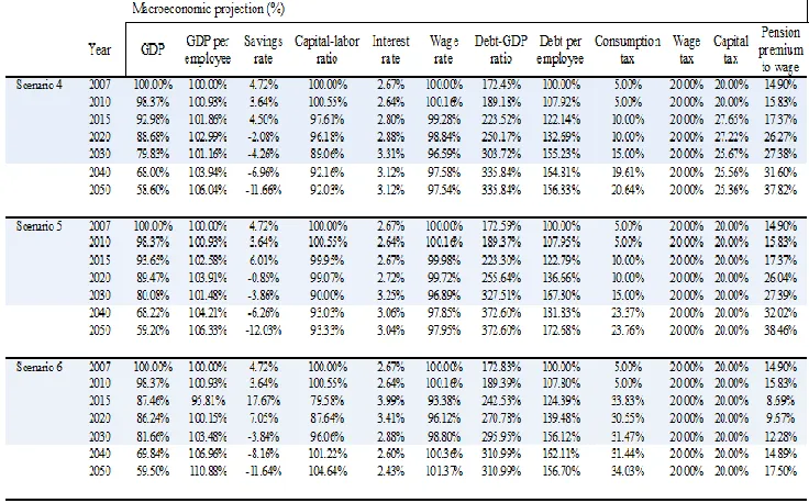
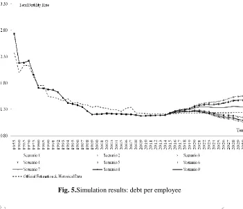
In this section, we will describe the simulation results reported in Table 4 and Figs. 2 to 6.
Demographic Projection and Macroeconomic Variables
First, we describe the demographic projection. Fig. 2 shows the population projection of future generations born in the period 2000–2050. The projection in Scenario 1 closely corresponds to the official estimation provided by theNational Institute of Population and Social Security Research (2008). In contrast to Scenario 1, Scenarios 2 to 5 (100% permanent child benefits increases) and 9
Fig. 4 shows the total fertility rate (TFR) from 1995 to 2030. The projections in Scenario 1 closely correspond to the official estimation provided by the National Institute of Population and Social Security Research (2007). Fig. 2 shows a TFR projection for all scenarios. For example, Scenario 5
shows the highest TFR with 1.55, followed by Scenario 3 with 1.48, in 2030.Fig. 3 shows a projection of the retired population ratio from 2010 to 2050. The projection in Scenario 1 closely corresponds to the official estimation provided by the National Institute of Population and Social Security Research (2007). In comparison to Scenario 1, the 2030 retired population ratio in
Scenarios 2 to 5, with permanent child benefit increases, decreases between 0.33% of a point and 0.42% of a point. Similarly, the ratio in Scenario 9 decreases by 0.22% of a point, not a highly significant difference. Further, the 2050 retired population ratio in Scenarios 2 to 5, with permanent child benefit increases, decreases between 2.5% of a point and 2.0% of a point, compared to the other scenarios. Regardless of the long-term improvements, in the short term, it seems unlikely that the retired population rate will decrease to any significant degree in response to child-rearing benefits. Next, we simply explain the projection from a macroeconomic perspective. As our model employs a life-cycle hypothesis, the savings rate is highly influenced by the aging population. Looking at the transition of macroeconomic variables shown in Table 4, all scenarios show a decrease in the savings rate between 2010 and 2050, compared to the 2007 rate of 4.72%. However, in comparison to Scenario 1, Scenarios 2 (child benefits expansion financed by consumption tax, and permanent child benefits increases), 4 (funded by capital income tax), 5 (funded by government debt), and 6 (50% reduction of the aggregated pension premium by increasing consumption tax) show a rise in the savings rate in 2030. Further, Scenarios 2 to 9 show a rise in the savings rate in 2050, as compared to Scenario 1.Finally, the factor price shows a stable transition in all scenarios, fluctuating between the interest rates of 2.43% (wage rate) and 3.99% (93.38% to 101.37%). In general, increased child benefits lead to more births, creating a greater workforce. However, an expanded workforce will lower the capital-labor ratio, possibly increasing the interest rate while simultaneously restraining the wage rate. Table 4 shows Scenarios 2 to 5 (permanent child benefits increases) reflecting a lower capital-labor ratio for 2030 than that of Scenario 1, along with lower GDP and GDP per employee. On the other hand, pension and fiscal reforms, as implemented in Scenarios 6 through 9, result in a higher capital-labor ratio, GDP, and GDP per employee.
Fiscal Variables
shows more improvement in Scenarios 7 to 9 than in Scenario 1. In particular, the public debt-to-GDP ratio after 2035 is projected at roughly 311% in Scenario 1, 281% in Scenario 7, 261% in Scenario 8, and 272% in Scenario 9.On the other hand, Scenarios 2 (child benefits expansion financed by increase in consumption tax), 3 (increase in wage tax), 4 (increase in capital income tax), and 5 (child benefits expansion financed by government debt) are worse in terms of debt per employee in comparison to Scenario 1; Scenarios 2 to 4 show increased interest due to the lower capital-labor ratio and Scenario 5 shows increased public debt due to the lower capital-labor ratio and the issue of government bonds to fund child benefits. Therefore, the public debt-to-GDP ratio after 2035 is projected at roughly 327% in Scenarios 2, 320% in Scenario 3, 335% in Scenario 4, and 372% in Scenario 5.The tax changes in Table 4 also show that the funding required for increased child benefits ranges from 2.12% to 3.44% in Scenario 2 (consumption tax funding), 2.40% to 3.12% in Scenario 3 (wage tax funding), and 5.36% to 7.65% in Scenario 4 (capital income tax funding).
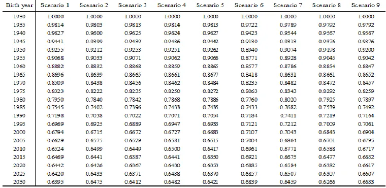
Welfare
effect of child-rearing cost on the welfare of the generation. In addition, among Scenarios 2 to 5, the welfare of the generations born in the period 1955 to 1980 is lowest in Scenario 2 (child benefits expansion financed by consumption tax). An additional tax on the retired generation’s consumption in the early stage after the child benefits expansion of Scenario 2 presents less distortion as it works as a lump-sum tax. This indicates that child benefits expansion funded by consumption tax results in an intergenerational income transfer from the retired to the younger generation.
On the other hand, the welfare for the generation born in 2075 is the highest in Scenario 9 (accelerated fiscal reform and child benefits expansion). The next highest figure is for Scenario 4 (child benefits expansion financed by capital income tax), followed by Scenario 5 (financed by government debt), Scenario 2 (financed by consumption tax), and Scenario 3 (financed by wage tax), in that order. All these scenarios have child benefits expansion. The sixth highest figure is that for Scenario 6 (maintains half of the pension premium through VAT), followed by Scenario 7 (pension benefits cut by 10% and child benefits expansion), Scenario 8 (accelerated fiscal reform), and, finally, Scenario 1, ranking ninth (baseline). All these scenarios (except Scenario 7) do not have child benefits expansion. Generally, public pension and accelerated fiscal reforms have the pressure of rising capital-labor ratio in the long period. In our model, while increased capital-labor ratio improves lifetime wage, it also increases child-rearing cost. Then, if the positive effect of improved lifetime wage is overshadowed by the negative effect of increased child-rearing cost, the welfare of future generations does not improve. The above order of the welfare for the generation born in 2075 indicates this mechanism, except for in Scenario 9. On the other hand, child benefits expansion leads to more births, creating a greater workforce, and has the pressure of reducing capital-labor ratio in the long run. This mitigates the negative effect of increased child-rearing cost. In addition, in our model, each generation obtains the welfare gain from more births. Therefore, the welfare for the generation born in 2075 is higher in Scenarios 2 to 5 and 9, as compared to in other scenarios6.Placing the highest importance on the welfare of future generations, Scenario 9 (accelerated fiscal reform and child benefits expansion) stands out as the most desirable option.
Conclusion and Future Issues
In this paper, we presented an OLG model with multi-concurrent generations and endogenous fertility to analyze the effects of increased child benefits and reduced pension benefits on the welfare of the working and future generations. The following results were obtained through the analysis. First, we considered increased child benefits without pension and accelerated fiscal
6
In Scenario 7, the effect of public pension reform on capital-labor ratio is greater than the effect of child benefits expansion
on the same. Therefore, the welfare for the generation born in 2075 is lower in this scenario, as compared to in Scenarios 2
reforms. Among Scenarios 2 to 5, the welfare of future generations improved most through child benefits funded by capital income tax. This indicates that the best policy is to cover child benefits via capital income taxation, followed by government bonds, VAT, and wage taxation, in that order. We also looked at the existing method of accelerated fiscal reform. In this case, rather than fiscal reform alone, coupling increased child benefits and fiscal reform simultaneously improves the welfare of future generations more. In particular, according to our simulation, it stands out as the most desirable option. Public pension reform was also examined. We found that using consumption tax to partially fund the pension premium, rather than cutting pension benefits coupled with increasing child benefits, yields a higher welfare for future generations.
Finally, we would like to address some relevant topics for future research.
endogenize the externality of pay-as-you-go public pensions and (2) an attitude of regarding children as investments, not as consumption. Finally, enhancing the framework of analysis, for example, expanding it from a closed- to an open-economy model and incorporating uncertainties, will certainly stimulate further research.
REFERENCES
Atkinson, A.B. and J.E. Stiglitz, 1972. The structure of indirect taxation and economic
efficiency. Journal of Public Economics, 1: 97-119.
Atkinson, A.B. and J.E. Stiglitz, 1976. The design of tax structure: Direct versus indirect
taxation. Journal of Public Economics 6(1-2): 55-75.
Auerbach, A.J. and L.J. Kotlikoff, 1987. Dynamic fiscal policy. Cambridge: Cambridge
University Press.
Chamley, C., 1986. Optimal taxation of capital income in general equilibrium with infinite
lives. Econometrica, 54(3): 607-622.
Conesa, J.C., S. Kitao and D. Krueger, 2007. Taxing capital? Not a bad idea after all!
Nber.
Cremer, H. and F. Gahvari, 1995. Uncertainty, optimal taxation and the direct versus
indirect tax controversy. Economic Journal, 105: 1165-1179.
Diamond, P.A., 1965. National debt in a neoclassical growth model. American Economic
Review, 55(5): 1126-1150.
Hatta, T. and Y. Oguchi, 1999. The theory of public pension reform: Transform to funding
system. Nikkei Publishing, Inc. [in Japanese].
Hubbard, R.G. and K.L. Judd, 1986. Liquidity constraints, fiscal policy, and consumption.
Brookings Papers on Economic Activity, 1: 1-59.
International Monetary Fund, 2011. Raising the consumption tax in japan: Why, when,
how? Available from IMF Staff Discussion Note No. 2011/13.
Judd, K.L., 1985. Redistributive taxation in a simple perfect foresight model. Journal of
Public Economics, 28(1): 59-83.
National Institute of Population and Social Security Research, 2007. Population statistics
of japan [in Japanese].
National Institute of Population and Social Security Research, 2008. Available from
Population Projections for Japan: 2006-2055.
Oguro, K., J. Takahata and M. Shimasawa, 2009. Child benefit and fiscal burden: Olg
model with endogenous fertility. IPSS Discussion Paper Series 2009-E01.
Weinzierl, M., 2007. The surprising power of age-dependent taxes. Available from
http://www.econ.yale.edu/seminars/jr-fac/jf08/Weinzierl_JMP.pdff.
Whitehouse, E., 2007. Pensions panorama: Retirement-income systems in 53 countries.
The World Bank.
Table-1.Parameter values of the model
PARAMETER VALUE
Utility function
Time preference rate 0.01
Intertemporal elasticity of substitution 1/ 2.0
Weight parameter between number of children and consumption
0.84*
Production function
Technology progress 0.002
Capital share in production 0.3
Physical capital depreciation 0.05
Tax policy parameters
Wage tax
tw
20.0%Capital tax
tr
20.0%Consumption tax
tc
5.0%Pension benefit tax tp 10.0%
Pension policy parameters
National subsidy to pension sp 25.0%
Replacement ratio 50.0%
Other parameters
Child-rearing cost to net lifetime income
0 to 5 0.78%
6 to 10 0.46%
11 to 15 0.55%
16 to 20 0.58%
Childbearing possibility
1 to 5 3.0%
6 to 10 7.4% 11 to 15 7.0%
16 to 20 2.6%
Government subsidy to child-rearing cost 0.1
Age-wage profile 0
1
2
88.3 7.08 -0.146 j
p
g g=
Age limit for childbearing
M
40Age of retirement Q 65
Average life expectancy Z 85
* This parameter is fixed after year 2007.
Table-2.Year 2007 of the baseline scenario
OFFICIAL MODEL
National Income (% of GDP)
Private consumption 74.1% 81.8%
Government purchases of goods and services
21.0% 24.3%
Saving rate 3.1% 4.7%
Government Indicators
Pension premium to wage 14.9% 14.9%
Gross public debt (% of GDP) 170.6% 172.4%
Primary balance (% of GDP) -2.4% -4.3%
Tax revenues (% of GDP) 18.4% 19.8%
Other Indicators
Capital output ratio 2.9 4.4
Interest rate 1.7% 2.6%
Source: OECD Economic Outlook No. 84, 2008, and ―Annual Report on National Accounts,‖ the Japanese
SNA statistics (Cabinet Office).
* In each simulation scenario, we keep the outstanding government debt to GDP after 2035 at the same level,
by controlling consumption tax.
Table 4. Simulation results
Table-4. Simulation results (continued)
Fig-2.Simulation results: demographic projection of future generations
Fig. 4.Simulation results: total fertility rate
Fig. 6.Simulation results: welfare with equivalent variation
Additional Information Simulation results: welfare with equivalent variation