Article
1
Reconstruction of a segment of the UNESCO World
2
Heritage Hadrian’s Villa tunnel network by
3
integrated GPR, magnetic
−
paleomagnetic, and
4
electric resistivity prospections
5
Annalisa Ghezzi1,*, Antonio Schettino1, Pietro Paolo Pierantoni1, Lawrence Conyers2, Luca Tassi1,
6
Luigi Vigliotti3, Erwin Schettino4, Milena Melfi5, Maria Elena Gorrini6 and Paolo Boila7
7
1 University of Camerino – School of Science and Technology, Camerino, Italy; E-Mails:
8
[email protected] (A.S.); [email protected] (P.P.P.); [email protected] (L.T.)
9
2 Department of Anthropology, University of Denver, Denver, CO 80210, USA; E-Mail: [email protected]
10
(L.C.)
11
3 Istituto di Scienze Marine , CNR, Bologna, Italy; E-Mail: [email protected] (L.V.)
12
4 Instituto Andaluz de Ciencias de la Tierra, CSIC – Universidad de Granada, Spain; E-Mail:
13
[email protected] (E.S.)
14
5 Faculty of Classics - University of Oxford, Oxford, UK; E-Mail: [email protected] (M.M.)
15
6 Dipartimento di Studi Umanistici, Università degli studi di Pavia, Pavia, Italy; E-Mail:
16
[email protected] (M.E.G.)
17
7 Idrogeotec S.N.C. - Perugia - Italy; E-Mail: [email protected] (P.B.)
18
19
* Correspondence: [email protected] (A.G.); Tel.: +39−0737−402641
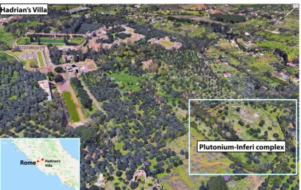
20
21
Abstract: The UNESCO World Heritage Hadrian’s Villa lies over the Colli Albani volcanic district
22
near Rome. Magnetic, paleomagnetic, radar, and electric resistivity surveys were performed in the
23
Plutonium–Inferi sector to detect buried buildings and outline a segment of the underground
24
system of tunnels that link different zones of the villa. In particular, a paleomagnetic analysis of the
25
bedrock unit allowed to accomplish an accurate geomagnetic field modelling and characterize the
26
archaeological sources of the magnetic field anomalies. We used a computer−assisted forward
27
modelling procedure to generate a structural model of the sources of the observed anomalies. The
28
intrinsic ambiguity of the magnetic field modelling was reduced with the support of ground
29
penetrating radar amplitude slices and an analysis of radar and electric resistivity profiles. The
30
bedrock lithology in this area is an ignimbrite tuff characterized by abundant iron oxides. The
31
high−amplitude magnetic anomalies observed in the Plutonium–Inferi area are due to strong
32
bedrock remnant magnetization and susceptibility contrasts between topsoil infill of cavities and
33
the surrounding tuff. The resulting magnetization model of the Plutonium–Inferi complex shows
34
that the observed anomalies are mostly due to the presence of tunnels, skylights and a system of
35
ditches excavated in the tuff.
36
Keywords: Archaeological geophysics; magnetic methods; ground penetrating radar; tunnel
37
detection; data integration.
38
39
1. Introduction
40
Hadrian’s Villa is a UNESCO World Heritage site near Rome (Figure 1). It was built starting
41
from 117−118 A.D. as one of the residences of the Roman Emperor Hadrian. Its location was chosen
42
for its scenic location, proximity to Rome, and the presence of four aqueducts directed to Rome.
43
44
Figure 1. Hadrian’s Villa Archaeological Site.
45
46
The villa lies over the Quaternary Colli Albani volcanic district, a ~600 ka to present
47
undersaturated K−rich magmatic province that is part of the ~250 km long peri−Thyrrhenian
48
volcanic belt [1]. The geological framework of this site consists of a complex volcano−sedimentary
49
succession made of ignimbrite sheets interposed with fall deposits and lava flows [2]. Irregularity in
50
geometry and thickness, as well as lateral facies variations and heterogeneous alteration of the
51
stratigraphic units are related to the paleotopographic control on the transport and depositional
52
mechanisms of the volcanic products. The outcropping lithology at Hadrian’s Villa consists of the
53
Pozzolanelle ignimbrite, the upper depositional unit of the Villa Senni eruption unit, which
54
represents the youngest (355 ka) mafic caldera−forming eruption of the Colli Albani [3,4]. The
55
Pozzolanelle unit is a chaotic, ignimbritic tuff massive deposit, ranging in thickness from < 2 to 40 m,
56
characterized by an ash matrix support texture abundant with phenocrystals (leucite, clinopyroxene,
57
and biotite), holocrystalline xenoliths, and reddish vesicular scoria clasts [5] (Figure 2).
58
The archaeological structures of this large villa include many monumental buildings and an
59
important underground network of tunnels that was created to link different parts of the complex
60
and, possibly, for the transport of supplies [6]. Nowadays only a small part of this network can be
61
travelled by non−speleologists. The first systematic description of Hadrian’s Villa was carried out by
62
Pirro Ligorio in the XVI [7]. Ligorio was the first to draw a complete map of the site and to attempt
63
an identification of the function of any specific feature of the villa by assigning names to its various
64
parts. One century later, Contini drew a more accurate map of the system of tunnels that run beneath
65
the villa on the basis of the earlier study by Ligorio [8]. His map was accepted without substantial
66
modifications by all the following draughtsmen, including Piranesi ([6] and references therein).
67
However, an important contribute to the characterization of the architectural elements of the villa
68
was provided at the beginning of the XIX by [9], who accurately described and recorded both
69
exposed structures and the accessible subterranean features (already mapped by earlier authors).
70
More recently, an accurate topographic survey of the network of tunnels was performed by [6]
71
(Figure 3), who divided the underground features in four categories according to their functionality.
72
The first category includes brick dressed cryptoportica and ambulacra. The second category
73
comprises underground tunnels for use of both pedestrians and carts, occasionally interrupted by
74
open−air segments. The third category includes underground pedestrian passages linking different
75
buildings of the villa, smaller in size than those of the former category. Finally, the last category
76
78
79
Figure 2. Stratigraphic section of the substratum of Hadrian’s Villa. The picture was taken along the Via
80
Tiburtina close to the highway entrance to Tivoli.
81
82
Figure 3. Hadrian’s Villa general plan (modified from [6]). PIC = Plutonium−Inferi complex; A = Accademia.
83
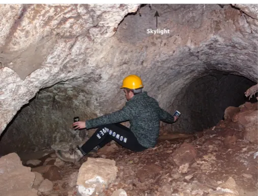
84
Despite the paramount archaeological importance of Hadrian’s Villa, there is a very scarce
85
record of published geophysical investigations at this site. Franceschini and Marras [10] applied for
86
the first time electric resistivity methods to reconstruct the layout of the subterranean tunnels in the
87
sector of the villa. A ground penetrating radar (GPR) survey of the area around the Plutonium−Inferi
89
complex (Figure 1) was undertaken in 2016 by a team of the British School at Rome [11] to facilitate
90
successive excavations in the context of a joint project of the universities of Oxford and Pavia [12].
91
The radar survey was performed using a 400 MHz antenna, which did not allow sufficient
92
penetration for investigating the system of tunnels that had been dug in the tuff units underlying the
93
Plutonium–Inferi area. The maximum penetration depth of this survey was ~100 cm, thereby the
94
resulting amplitude maps only showed archaeological features buried in the topsoil, and not the
95
cavities in the underlying rock formation. To date, the most used geophysical technique at Hadrian’s
96
Villa has probably been the laser scanner (an interesting example can be found in [13]). Finally, it is
97
worth mentioning the sophisticated surveying techniques (probes and robots) used in recent years
98
by the Centro Ricerche Speleo Archeologiche of Rome, which explored a segment of the
99
underground road system known as the “Strada Carrabile” [14].
100
We performed an integrated geophysical survey at one of the least known sectors of Hadrian’s
101
Villa, the Inferi−Plutonium complex (Figure 1), with the objective of reconstructing a segment of the
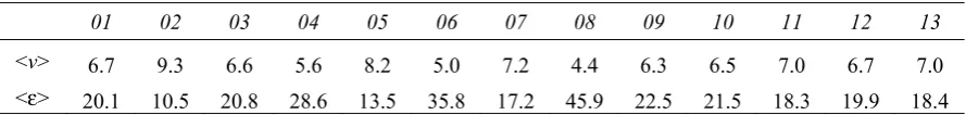
102
underground tunnel network in this area (Figure 4).
103
104
105
Figure 4. Tunnels in the Plutonium – Inferi complex.
106
107
The buildings in the Inferi−Plutonium area have been generally understood as related to the
108
belief of an after−life existence and the cult of death [15]. According to this hypothesis, that dates
109
back to the first explorations by Pirro Ligorio, the Inferi, a large ditch dug in the tuff, would
110
represent the River Styx and the entrance to the Underworld, while the Plutonium would be a
111
temple devoted to Pluto, king of the Underworld. The present study aims at detecting cavities in the
112
tuff units by combining several sources of data, obtained from different geophysical methods:
113
electric resistivity, magnetometry, GPR, paleomagnetism, and aerial photogrammetry. The whole
114
area was covered by the GPR survey, but because of the presence of fences or iron scraps, the
115
magnetic data were collected only in the central and western portion of the complex.
116
117
The strong magnetic susceptibility χ and natural remnant magnetization (NRM) of the tuff
118
units on which Hadrian’s Villa was built has amplified the contrast with the buried structures and
119
the cavities in the substratum, so that the corresponding magnetic anomalies reach amplitudes up to
120
~2200 nT. In a sense, the bedrock geology of this site is a unique example of a natural “amplifier” of
121
magnetic anomalies associated with archaeological features. Consequently, we used the magnetic
122
data set as the primary source for reconstructing the layout of the tunnel network by using a
123
technique of forward modelling, but the whole procedure and the results were constrained and
124
assessed, respectively, by the other sources of data. In particular, the integration with GPR data
125
allowed to extend the reconstruction beyond the area surveyed with magnetic methods, while both
126
magnetization model. In the next sections, we first discuss the various techniques used for the data
128
acquisition and processing, then we show how the different sources of data were integrated in order
129
to reconstruct the topology of the tunnel network underneath the Plutonium−Inferi area. Our results
130
confirm the presence of tunnels whose existence was already known, but also reveal the existence of
131
additional underground tunnels and of a system of ditches dug at the top of the tuff, which probably
132
served as irrigation channels.
133
2. Methods
134
Initially, magnetic, radar, and electric resistivity surveys performed in 2017–2018 had the
135
primary objective of assessing potential security issues during the excavations around the
136
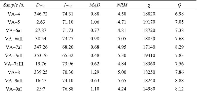
Plutonium−Inferi complex. In addition, paleomagnetic and precise topographic data were acquired
137
in view of the creation of a reliable magnetization model of the buried structures and cavities. Below
138
we describe in detail the acquisition and processing methods for each of the geophysical techniques
139
used in this survey.
140
2.1. GPR Data Acquisition and Processing
141
GPR data were acquired using a GSSI SIR 4000 system equipped with a 200 MHz antenna,
142
which in principle should have allowed sufficient penetration for investigating the system of tunnels
143
that had been dug in the tuff units underlying the Plutonium–Inferi complex. However, the soil of
144
this area includes abundant clays that formed by weathering of the volcanic substratum. In moist
145
conditions, these clays display strong electric conductivity and attenuation, thereby the maximum
146
depth of penetration did not generally exceed 2.5 m. GPR data were acquired using the following
147
basic parameters:
148
149
• Survey mode = Distance mode (with odometer)
150
• Scans/m = 50
151
• Samples/scan = 1024
152
• Range = 300 ns
153
• Bits/sample = 32
154
• Line spacing = 0.5 m
155
• Antenna = GSSI 5106, 200 MHz
156
157
To improve the coupling with the ground, the survey lines were travelled using three operators,
158
one at the console and two who drove the large 5106 antenna along the tracklines (Figure 5). Other
159
people were responsible for the setup of the survey geometry, for the GPS positioning, and for the
160
deployment of metric tapes. A local reference frame was established, in order to combine GPR data
161
coming from different areas. We divided the survey region in 13 areas (Figure 6) of variable
162
geometry. In all cases, the survey lines were travelled in bi–directional mode and the local
163
coordinates of the end points were recorded by an operator directly in the field. A set of 14 reference
164
points was established, with assigned local coordinates (
ξ
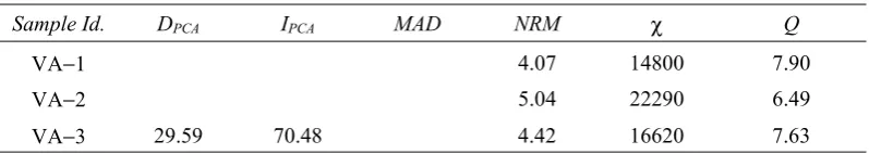
i,
ψ
i) and known geographic coordinates165
(
x
i,
y
i) obtained by GPS measurements and expressed in the UTM 33 reference frame. A computer166
algorithm then calculated the best–fitting rigid transformation from local coordinates to UTM by
167
weighted least squares minimization of corner location errors relative to the measured GPS
168
locations. The best–fitting orientation of the local reference frame relative to the UTM datum is
169
illustrated in Figura 5, along with the GPS reference points. In all cases, the misfit between reference
170
point locations and best–fitting UTM coordinates resulted to be less than 1.5 m. The resulting data
171
set underwent the following basic processing steps:
172
173
• Band pass filtering (~100 – 300 MHz)
174
• Background removal
175
• Migration
176
• Normalization
178
• Equalization
179
• Knitting
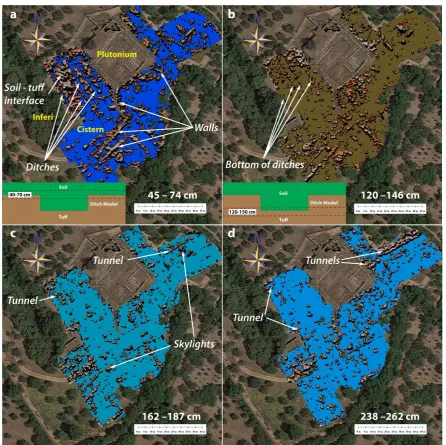
180
181
182
Figure 5. GPR system used to investigate the area and arrangement of operators.
183
184
185
Figure 6. System of 14 GPS points used to define the local reference frame (yellow dots) and GPR
186
survey areas (red lines). The direction of the survey lines is indicated by the white arrows. The
187
coordinate axes (x,y) show the best–fitting reference frame through the assigned GPS points.
188
189
To perform the data migration, we searched and fit reliable hyperbolae for each area. Then,
190
laterally homogeneous velocity models were built subdividing the substratum into horizontal
191
layers, different for each area. The average velocity, <v>, and relative dielectric permittivity, <ε>, of
192
each area of Figure 6 is listed in Table 1. These parameters were calculated over a reference two−way
193
travel time (TWTT) interval T = 100 ns starting from the pairs (Tk,vk) provided by the velocity
analysis, Tk and vk being the TWTT to the bottom of layer k and the corresponding velocity through
195
the same layer, respectively:
196
(
1)
1
k k k k
v
v T
T
T
−=
−
(1)197
2
2
c
v
ε =
(2)198
199
where c = 30 cm ns−1 is the speed of light.
200
201
Table 1. Average velocity (in cm ns−1) and dielectric constant of the 13 areas of Figure 6
01 02 03 04 05 06 07 08 09 10 11 12 13
<v> 6.7 9.3 6.6 5.6 8.2 5.0 7.2 4.4 6.3 6.5 7.0 6.7 7.0
<ε> 20.1 10.5 20.8 28.6 13.5 35.8 17.2 45.9 22.5 21.5 18.3 19.9 18.4
202
At the next step, 30 cm thick amplitude slices were generated for all the 13 areas, with a 50%
203
overlap between successive slices. From this data set, we chose four meaningful time slices that were
204
representative of shallow, intermediate, and deep-burial depths. These slices were normalized to
205
reduce amplitude differences associated with diverse conditions of the ground. To obtain a mosaic
206
of the 13 areas at each depth, the knitting procedure of the amplitude slices required an equalization
207
step to ensure continuity along the edges of adjacent areas.
208
2.2. Magnetic Field Intensity Acquisition & Processing
209
Total field magnetic intensities were collected using a Geometrics G–858 caesium vapor
210
magnetometer. The whole survey area was divided in 10 rectangles having variable dimensions,
211
which were assembled at the end of the processing in the UTM 33N reference frame (Figure 7).
212
213
214
Figure 7. Area covered by the magnetic survey.
215
216
The magnetic data were acquired at 10 Hz frequency (corresponding to an average 11 cm
217
distance between successive readings) along bi–directional survey lines equally spaced 0.5 m. All the
218
and the data underwent standard pre–processing consisting into despiking and decorrugation
220
procedures. Then, the total field data of each area were decorrugated and combined into a mosaic
221
through an equalization and knitting procedure that ensured continuity along the edges of adjacent
222
areas.
223
2.3. Paleomagnetic Acquisition & Processing
224
We sampled 13 cores from the Pozzolanelle unit by using a portable drill. The cores were
225
oriented using a magnetic compass. The sampling was integrated by soil specimens of the
226
substratum in the survey area. The measurements were carried out in the paleomagnetic laboratory
227
of ISMAR−CNR in Bologna. The NRM of the tuff was acquired by these rocks at the time of their
228
deposition and cooling. Therefore, it is an expression of the Earth’s magnetic field direction at that
229
time. The induced magnetization of the tuff and soil units depends from their magnetic
230
susceptibility and is directed as the Earth’s magnetic field at survey time in the Plutonium−Inferi
231
area. Both the tuff NRM and the magnetic susceptibility of the tuff and soil units represent
232
fundamental quantities that will be used in the subsequent magnetic field modelling procedure.
233
To determine the magnetic minerals that are responsible for the tuff remnant and induced
234
magnetization components, we applied a Mössbauer spectroscopy technique. This is a powerful
235
method that can be used for the identification of iron−bearing minerals when the magnetic
236
properties of the material are due to a mixture of ferromagnetic minerals. In particular, this
237
technique is very useful when the sample contains minerals with similar magnetic properties, not
238
easily distinguishable using traditional rock magnetic methods, or when weakly magnetic minerals
239
like hematite are mixed with minerals characterized by stronger magnetization, for example
240
magnetite [16]. The absorption spectrum of the Pozzolanelle ignimbrite is shown in Figure 8. The fit
241
to these data is dominated by three strong paramagnetic doublets, but also includes a broad central
242
singlet indicative of the presence of small grains of superparamagnetic iron oxides above their
243
blocking temperature. Finally, the observed spectrum shows four weaker ferromagnetic sextets. The
244
Mössbauer parameters of the doublets are characteristic of Fe+3 or Fe+2 in octahedral coordination, as
245
it is often observed in the spectrum of biotites, but much more likely arise from the presence of
246
superparamagnetic iron oxyhydroxides such as goethite or ferrihydrite, which are common
247
alteration products in volcanic rocks. These components account for 64% of the spectral area, while
248
another 13% is represented by the superparamagnetic iron oxides. The remaining four ferromagnetic
249
components suggest the presence of maghemite (9%), non−stoichiometric magnetite (7%), and
250
possibly superparamagnetic hematite just below the blocking temperature (8%). Although the
251
interpretation of the latter component is only a tenable hypothesis, it is supported by the large
252
amount of hematite visible on the sample (see Figure 2) and by a preliminary X−ray diffraction
253
analysis performed on the specimen.
254
In order to obtain the characteristic remnant magnetization (ChRM) of the rock unit, a stepwise
255
alternating field (AF) demagnetization process was applied to the collected samples. The bulk
256
volume susceptibility χ was measured using a Bartington MS2 susceptibility meter and the results
257
were used to calculate the induced magnetization. The rock exhibits a single component of
258
magnetization with only a minor viscous magnetization easily removed after 5 mT of AF field
259
(Figure 9a).
260
The results listed in Table 2 show that these rocks have strong NRM and a relevant induced
261
magnetization, in agreement with the results of Mössbauer spectroscopy. From these data, we obtain
262
an average volume magnetic susceptibility χ
=
18126.92×10−6 SI units. Therefore, assuming a263
reference field vector F with intensity F = 46,489.2 nT and direction (D0 = 3.14°, I0 = 58.16°) on Feb 9th
264
2018 at 41.937567° N, 12.779273° E, it results a mean induced magnetization MI = (χ/μ0)F = 0.67 A m–1.
265
The average NRM intensity results to be MR = 4.82 A m–1 (13 specimens mean) with a mean direction:
266
(D = 4.1°,I = 72.8°) (10 samples average), the statistical parameters k and α95 being respectively: k
267
=141.3 and
α
95 = 4.1° (Figure 9b). Taking into account of the rapid deposition and cooling of the268
pyroclastic flow, this paleomagnetic direction can be considered as representative of the
269
271
Figure 8. Room temperature 57Fe Mössbauer spectrum of a Pozzolanelle unit specimen. Dots are
272
original data points, black line is the best fitting envelope of the eight spectral components.
273
274
275
Figure 9. (a) AF demagnetization plot; (b) Paleomagnetic directions (red dots) with resulting mean (green dot).
276
277
Table 2. Results of palaeomagnetic analysis
Sample Id. DPCA IPCA MAD NRM χ Q
VA−4 346.72 74.31 0.88 4.58 18820 6.98
VA−5 2.63 71.10 1.06 4.71 19170 7.05
VA−6aI 27.87 71.73 0.77 4.81 18720 7.38
VA−6aII 38.54 73.77 0.98 5.05 18850 7.68
VA−7aI 347.26 68.20 0.68 4.95 17140 8.29
VA−7aII 353.76 65.32 0.48 5.30 19410 7.83
VA−7aIII 19.76 73.96 0.62 4.84 18360 7.56
VA−8 339.25 70.30 1.29 5.00 18250 7.86
VA−9aII 16.47 74.10 0.63 5.65 18240 8.88
Table 2. Continued
Sample Id. DPCA IPCA MAD NRM χ Q
VA−1 4.07 14800 7.90
VA−2 5.04 22290 6.49
VA−3 29.59 70.48 4.42 16620 7.63
DPCA = NRM declination from principal components analysis [°deg]
IPCA = NRM inclination from principal components analysis [°deg]
MAD =Maximum angular deviation from mean [°deg]
NRM = Remnant magnetization intensity [A m–1] χ = Magnetic susceptibility [×10–6]
Q = Koenigsberger ratio
2.4. Electric Resistivity Acquisition & Processing
278
Electrical resistivity data were acquired using a Geopulse Tigre 128 resistivity meter. The
279
acquisition parameters were set to optimize input current, shape of the current signal input, number
280
of averaged potential readings, and sampling time. This instrument is able to automatically cancel
281
the spontaneous potentials that are eventually generated in the ground and that, in the case of small
282
drops in potential during the measurements, would have been one of the major sources of noise.
283
Before carrying out the measurements, a control test was carried out on the value of the contact
284
resistance between the electrodes and the ground, accepting a resistance value lower than 2000 Ω.
285
We performed ten resistivity acquisitions using 32 electrode spreads. Eight 2D geoelectric profiles
286
out of ten were created using a Wenner−α geometry and 1 m electrode separation, while the
287
remaining two profiles were acquired using a dipole−dipole configuration with 2 m electrode
288
separation. The former array is relatively sensitive to vertical changes in subsurface resistivity below
289
the center of the array and less sensitive to horizontal changes in the subsurface resistivity. The
290
advantage is that a smaller amount of acquisitions is necessary to build a pseudosection. For each
291
profile, the repetition time interval of the square sampling wave was set to 2.8 s, while the number of
292
averaged readings for the estimate of the resistivity was set to 4.
293
The resulting data set was processed using the software Res2DInv (Geotomo Software), and a
294
search criterion based on the minimum data heterogeneity [17]. In the initial pre−inversion step, we
295
analyzed the data quality of each electric resistivity profile through a test inversion and displayed
296
the resulting root mean square (rms) errors. The subsequent inversion step adopted a strategy based
297
on a 10% increase in the thickness of the layers as the depth increased.
298
2.5. Aerial Photogrammetry
299
We used unmanned aerial vehicle (UAV) photogrammetry to create a digital terrain model
300
(DEM) of the Plutonium−Inferi complex (Figure 10) according to the Structure from Motion technique.
301
The UAV was a DJI Phantom 4 equipped with an RGB visible light camera, flying at 40 m altitude at
302
~4 m/s speed. A GPS supported by regional network was used for georeferencing a set of ground
303
control points and scale the aerial photogrammetric survey. The bare−Earth extraction from the
304
DSM was accomplished using the software Photoscan and a point clouds segmentation and
305
classification algorithm. The final DEM was created using the software Thopos (Studio Tecnico
306
Guerra) and covered an area of 30230 m2 with a pixel size of 0.0456 × 0.0456 m2.
309
Figure 10. UAV orthophoto of the study area (Plutonium−Inferi complex).
310
3. Results
311
We compiled four depth slices, corresponding to the intervals: 45–74 cm, 120–146 cm, 162–187
312
cm, and 238–262 cm. They are shown in Figure 11. In these maps, the presence of reflectors is
313
indicated by brown colours while their absence is shown in green or blue. The colour intensity is
314
always proportional to the corresponding reflection amplitude. However, it is worth noting that the
315
nature of the reflectors cannot be established by the mere visual inspection of these depth slices. It
316
can be only determined after an analysis of individual radar profiles. The interpretation of
317
amplitude slices is complicated by the fact that structures (and associated reflectors) that are inclined
318
with respect to the Earth surface may be subdivided between different slices and slightly displaced
319
with respect to each other. Excluding long reflectors associated with the contact between
320
stratigraphic units, in general strong localized reflections are produced by: 1. cavities, 2. water–
321
saturated soil, 3. walls and other building remains, 4. modern public utilities, and 5. modern artifacts
322
[18]. However, significant reflections may also be locally associated with partial decoupling of the
323
antenna (for example, as a consequence of a ground surface irregularity), scatterers (e.g., stones), and
324
nearby metals (e.g., fences). All the radar profiles in the data sets 01 through 13 (Figure 6) were
325
analyzed individually to give a precise characterization of the sources of each relevant feature
326
detected on the amplitude slices.
327
An interesting feature of the 45−74 cm depth slice (Figure 11a) is represented by linear regions
328
characterized by the lack of reflections. An analysis of profiles through these regions shows that they
329
correspond to ditches excavated at the top of the tuff layer, according to the conceptual model
330
shown at the bottom of Figure 11a. This interpretation is in agreement with the 120−146 cm slice
331
333
334
Figure 11. GPR amplitude maps for the depth intervals : (a) 45–74 cm (12−20 ns); (b) 120–146 cm (33−41 ns); (c)
335
162–187 cm (47−55 ns); (d) 238 – 262 cm (72−80 ns).
336
337
Both the 45−74 cm and 120−146 cm amplitude slices show the presence of structures that can be
338
interpreted as walls [12], but an analysis of these features goes beyond the scope of this paper. The
339
next 162−187 cm and 238−262 cm depth slices (Figure 11c−d) show the first evidence of structures
340
that can be interpreted as tunnels and skylights. This interpretation will be discussed in the next
341
section.
342
The magnetic field intensity grid obtained by the procedure described in the previous section
343
was used to create a magnetic anomaly grid (Figure 12a) according to the method developed by [19].
344
In particular, the magnetic anomalies ΔT were calculated by subtraction of a 3th degree polynomial:
345
346
(
) ( )
≤ +
− =
Δ
N m n
m n m nb x y
a y
x T N y x
T , ; , (3)
347
348
where T(x,y) are observed total field intensities, N = 3 is the polynomial degree of the reference
349
field, and the coefficients an and bm were calculated by statistical regression on the observed data.
352
Figure 12. (a) The magnetic anomaly map of the Plutonium-Inferi complex; (b) Uncertainty grid.
353
354
Figure 12a shows that the magnetic anomalies observed in the Plutonium–Inferi area have very
355
strong intensity. They are mostly due to air−filled and soil−filled cavities embedded in the highly
356
magnetized bedrock. In particular, the strong circular negative anomalies visible in the map are the
357
magnetic expression of the buried skylights observed on the GPR amplitude slices (Figure 11c−d),
358
while the narrow linear negative anomalies reveal the presence of the ditches excavated in the tuff
359
layer (Figure 11a−b). Differently from the maps in Figure 11, the unique visual evidence of tunnels in
360
the magnetic anomalies consists into a small 20 m stripe of negative amplitudes aligned with the
361
sequence of skylights (Figure 12a).
362
The uncertainty ε associated with the magnetic anomaly map of Figure 12a is shown in Figure
363
12b. It was obtained by the following expression [19,20]:
364
365
( )
2 1/30
, p / 2
x y T
ε = ε ∇ + ε (4)
366
367
where ⏐∇T⏐ is the analytic signal of the observed total field intensities, εP is the maximum
368
estimated positioning error, and ε0 is the background uncertainty associated with the statistical
369
regression of the observed total field intensities to a polynomial surface [19]. On the basis of the field
370
conditions, we estimated a maximum positioning error εP = 0.15 m, while the regression uncertainty
371
resulted to be ε0 = 5.29 nT. Figure 12b shows that the highest uncertainty values are found where the
372
magnitude of the anomalies exceeds 1000 nT. An estimate of the uncertainty associated with the total
373
field observations is necessary for the modelling of the magnetic sources (see below) to avoid
374
overfitting of magnetic anomalies that have been calculated on the basis of a magnetization model to
375
anomalies that are associated with observed total field intensities at a level of accuracy exceeding the
376
actual uncertainty.
377
We also generated the radially averaged power spectrum [21] of the magnetic anomaly grid,
378
with the primary objective of checking that the ensemble with the highest slope had a depth
379
compatible with the maximum expected depths of the archaeological features [19,20,21]. However,
380
this kind of analysis also provides a quantitative estimate of the average depths associated with the
381
statistical ensembles that constitute the magnetic sources, which will be used in the subsequent
382
procedure of forward modelling. The radially averaged power spectrum of Figure 13 shows the
383
existence of four ensambles at different depths, which are in perfect agreement with the observed
384
archaeological features in the Plutonium−Inferi area. The deepest set of sources can be found at
385
depths exceeding 2.6 m and is most probably due to the presence of tunnels, while ditches dug at the
386
remains of archaeological features that are present at shallower depths (< 0.5 m) are represented by
388
the two ensambles at 0.42 m and 0.26 m (Figure 13).
389
390
391
Figure 13. Radially averaged power spectrum of the magnetic anomalies in Figure 12a.
392
393
We performed a quantitative modelling of the magnetic anomalies [19,20], with the objective of
394
assigning precise locations to tunnels and ditches but excluding from the model the much smaller
395
signal associated with walls and other shallow features. As mentioned above, Hadrian’s Villa lies on
396
a substratum composed by an ignimbrite tuff massive deposit with very high magnetic
397
susceptibilityχand strong NRM. In this area, the tuff is also covered by a ~0.5 m layer of very
398
magnetic soil with susceptibility χ0 = 9500×10–6 SI units. The magnetization model shown in Figure
399
14 does not include archaeological features buried in this topsoil layer, thereby the fit between
400
calculated and observed anomalies is rather coarse, although it explains most of the high−amplitude
401
anomalies observed in this area. These two layers were modelled as slabs underneath the whole area
402
at depths 0.5−5 m and 0−0.5 m respectively. To model empty tunnels and skylights in the tuff, we
403
used rectangular prisms and cylinders, respectively, embedded in the tuff unit and with opposite
404
magnetization parameters: MR = −4.82 A m−1, D = 4.1°, I = 72.8°, χ = −18127 ×10–6 SI units. Similarly, to
405
create a model of soil−filled ditches carved in the tuff, we defined vertical prisms that overlapped
406
the uppermost part of the tuff layer with opposite NRM and susceptibility χ = χ0−18127×10–6 SI units
407
= −8627×10–6 SI units.
410
Figure 14. Magnetization model (yellow lines with barbs) of the tunnels, skylights and ditches detected in the
411
Plutonium-Inferi area on a shaded magnetic anomaly map.
412
4. Discussion
413
The data presented in the previous section allowed us to draw a realistic layout of the tunnel
414
network beneath the Plutonium−Inferi area. We used a computer−assisted procedure of forward
415
modelling to generate a magnetization model that explained the observed anomalies in the western
416
portion of the complex. An example of the accuracy of the magnetization model in Figure 14 in
417
explaining the observed anomalies is illustrated in Figure 15. The very good fit between observed
418
and theoretical anomalies in the two profiles suggests that the voids and soil−filled structures in the
419
tuff are responsible for most of the magnetic signal in this area, while the walls and other artifacts
420
embedded in the topsoil account only for a minor contribution to the observed data.
421
The magnetization distribution shown in Figure 14 was constrained and complemented by GPR
422
and electric resistivity data, because of the intrinsic ambiguity of potential field data modelling. A
423
meaningful example of the data integration procedure is illustrated in Figure 16, which shows a
424
correlation between the three data sources. The GPR profile of Figure 16 shows a large hyperbole at 7
425
m offset, generated by a metallic lid covering the skylight [6]. The presence of a 5 m large tunnel
426
flanking the Inferi (Figure 3) is confirmed by the very high resistivity region (in brown) on the
427
revealed by the low resistivity regions (in blue), by the interrupted radar reflections of the soil−tuff
429
interface, and by the displaced reflections associated with their bottom surface. Finally, the GPR
430
profile also shows the bottom of a 180 cm high void space (20−32 ns) above the soil that partially fills
431
the tunnel .
432
433
434
Figure 15. Magnetic profiles across the ditches, skylights, and the main tunnel of areas M15, M16, and M18 of
435
Figure 7 (shapes bounded by black lines). The two profiles show observed and calculated anomalies as black
436
and blue lines, respectively, while the grey area shows the local uncertainty.
437
438
439
Figure 16. Correlation chart between magnetic, radar, and resistivity data showing ditches, skylights, and the
440
main tunnel in areas M15, M16, and M18 of Figure 7. From top to bottom: magnetic profile along the trace A−A′
441
of Figure 15, conceptual magnetization model, radar profile, and projected electric resistivity profile. C = cover
442
The magnetization model in Figures 15 and 16 does not necessarily provide a complete
444
representation of the underground structures. For example, some ERT and GPR profiles parallel to
445
the one shown in Figure 16 suggest the presence of a narrow tunnel below the irregular ditch
446
running parallel to the Plutonium. Further surveys are necessary to confirm the existence of such
447
deep structure. Instead, the pattern of ditches illustrated in Figure 15 provides a very good
448
representation of the system of irrigation ducts and planting pits described by [22] and indicates the
449
presence of a garden surrounding the Plutonium.
450
The tunnel crossing areas M15, M16, and M18 (Figure 14) corresponds to the main Strada
451
Carrabile [14] (see Figure 3). This important 5 m large underground pathway continues in SSE
452
direction towards areas M20−M22, where it reaches a shallower depth generating a strong linear
453
negative magnetic anomaly, clearly visible along the skylights alignment (Figure 14). Figure 17
454
shows radar and ERT profiles supporting this magnetization pattern. Beyond the modern fence that
455
surronds the archaeological park, the Strada Carrabile is linked southwards to a large four−sided
456
system of tunnels known as the “Grande Trapezio” (Figure 3) [6].
457
458
459
Figure 17. ERT and GPR evidence of the main tunnel and skylights in area M22 of Figure 7.
460
461
Two important findings in this sector were: 1. the identification on a series of radar profiles of
462
an entrance to the main tunnel (Figure 18), and 2. the detection on three ERT profiles of a deep
463
transversal tunnel running below the Strada Carrabile (Figure 19). The profiles in Figure 18 show
464
clear evidence of two retaining walls flanking a downgoing, 1.7 m large, stairway or ramp
465
orthogonal to the Strada Carrabile, similar to the one described by [10] for the Accademia sector. The
466
ERT profile of Figure 19 shows a very high resistivity region that can be interpreted as a tunnel
467
having the ceiling at ~4.5 m depth. Such a deepness can explain why the segment of Strada Carrabile
468
located in area M22 raises towards the surface. In fact, it is likely that the deep transversal tunnel
469
was built at an earlier time, possibly an aqueduct of Republican age [6], preceding the construction
470
of Hadrian’s Villa.
471
472
474
475
Figure 18. GPR evidence of a stairway entrance to the main tunnel. The existence of two retaining walls is
476
evident on four radar profiles, which also show steps or a ramp at increasing depth. The stairway location is
477
indicated by the parallel red lines on the background 162–187 cm GPR amplitude slice (Figure 11c).
478
479
480
Figure 19. ERT evidence of a large deep transversal tunnel.
481
482
The eastern portion of the Plutonium−Inferi complex has not been investigated by magnetic
483
methods due to the presence of fences. However, both GPR and electric resistivity data revealed
484
interesting features of this sector. The ERT and GPR profiles of Figure 20 show evidence of a couple
485
of tunnels in the direction of the northeastern slope, which could represent a way out from the villa
486
towards the ancient Via Tiburtina. The radar profiles also show the presence of a skylight and a well
487
filled by a jumbled assemblage of stones. The two tunnels had never been documented in previous
488
maps. Figure 20 also shows an ERT profile with evidence of cavities flanking the eastern wall of the
489
491
492
Figure 20. ERT and GPR evidence of a couple transversal tunnels linking the Plutonium to the northwestern
493
slope. W is interpreted as a well, S is a skylight.
494
495
The map in Figure 21 combines the results presented so far, based on magnetic field modelling
496
and the integration of radar and resistivity data. In addition to the structures discussed above, it
497
shows a portion of a large ditch having circular shape and 32 m diameter, excavated at the soil-tuff
498
interface. There is some archaeological evidence that this structure served to accumulate and
499
distribute water, as it is confirmed by the finding of lead pipes during the recent excavations [12].
500
Together with the evidence of a garden, the presence of this structure and possibly that of a large
501
pool within the circular area point to a reconstruction of the Plutonium−Inferi complex that included
502
a monumental primary entrance to the Plutonium [12].
503
505
Figure 21. Final model for the tunnel network in the Plutium−Inferi area. Ditches are also displayed. Excavated
506
walls are displayed in white [12].
507
508
5. Conclusions
509
In this paper, we have presented a model of the tunnels running beneath the Plutonium−Inferi
510
area and a description of buried structures that were presumably part of a garden. The latter features
511
consist into a system of ditches that were carved on the top of the tuff. The proposed pattern of
512
buried structures is based on the forward modelling of magnetic anomalies, supported by GPR
513
amplitude slices and the analysis of individual GPR and ERT profiles. In addition to the primary
514
goal of delineating the precise location of known tunnels across the Plutonium−Inferi area, we found
515
evidence of: a) an entrance to the main underground tunnel; b) a pair of previously unknown parallel
516
tunnels in the eastern sector, which probably represent a way out from the villa towards the Via
517
Tiburtina, and c) a previously unknown deep transversal tunnel in the western sector, probably an
518
aqueduct of Republican age.
519
520
Author Contributions: Conceptualization of the methodology, design of the field experiments, design of the
521
modelling software, formal analysis of magnetic and GPR data, and integration of the various sources of data,
522
A.G. and A.S.; interpretation of radar profiles, A.G. and L.C.; acquisition, treatment, and formal analysis of
523
paleomagnetic data, L.V. and A.G.; acquisition and formal analysis of electric resistivity data, L.T. and P.B.;
524
mineralogical analysis of rock samples, E.S.; acquisition and formal analysis of aerial photogrammetry data,
525
P.B.; GPS data acquisition and design of the field survey geometry, A.S., P.P.P., and A.G.; geological data
526
original draft preparation, A.G.; review and editing, A.S., M.M., L.T., E.S., L.V., and L.C.; project supervision,
528
A.S.; project coordination, M.E.G.
529
Funding: This research was funded by the Università degli Studi di Camerino, grants FAR Schettino 2016−2018
530
and FAR Pierantoni 2016−2018, and by the University of Oxford, Eugene Ludwig Fund, New College.
531
Acknowledgments: The authors are grateful to the Director of the Villa Adriana and Villa d’Este, Dr. Andrea
532
Bruciati, for kindly allowing to survey the archaeological area and to Drs. Benedetta Adembri and Sabrina
533
Pietrobono for facilitating the research on site. We are also grateful to Francesco Ferruti and the students that
534
helped us in the data acquisition. Finally, we thank Alessandro Bertani for his help in the acquisition and formal
535
analysis of aerial photogrammetry data.
536
Conflicts of Interest: The authors declare no conflict of interest. The funders had no role in the design of the
537
study; in the collection, analyses, or interpretation of data; in the writing of the manuscript, or in the decision to
538
publish the results.
539
540
References
541
542
1. Funiciello, R.; Giordano, G.; De Rita, D. The Albano maar lake (Colli Albani Volcano, Italy): recent volcanic
543
activity and evidence of pre-Roman Age catastrophic lahar events.J. Volcanol. Geotherm. Res. 2003, 123,
544
43-61.
545
2. Giordano, G.; De Benedetti, A.A.; Diana, A.; Diano, G.; Gaudioso, F.; Marasco, F.; Miceli, M.; Mollo, S.;
546
Cas, R.A.F.; Funiciello, R. The Colli Albani mafic caldera (Roma, Italy): Stratigraphy, structure and
547
petrology. J. Volcanol. Geotherm. Res.2006, 155, 49-80.
548
3. Soligo, M.; Tuccimei, P. Geochronology of Colli Albani volcano. In The Colli Albani Volcano; Funiciello, R.,
549
Giordano, G. Eds.; Special Publications of IAVCEI, 3. The Geological Society of London, London, 2010; pp.
550
154-196.
551
4. Vinkler, A.P.; Cashman, K.; Giordano, G., Groppelli, G. Evolution of the mafic Villa Senni caldera-forming
552
eruption at Colli Albani volcano, Italy, indicated by textural analysis of juvenile fragments. J. Volcanol.
553
Geotherm. Res.2012, 235-236, 37-54.
554
5. Watkins, S.D.; Giordano, G.; Cas, R.A.F.; De Rita, D. Emplacement processes of the mafic Villa Senni
555
Eruption Unit (VSEU) ignimbrite succession, Colli Albani volcano, Italy. J. Volcanol. Geotherm. Res. 2002,
556
118, 173-203.
557
6. Salza Prina Ricotti E. Criptoportici e Gallerie sotterranee di Villa Adriana nella loro tipologia e nelle loro
558
funzioni. Publications de l'École Française de Rome1973,14(1), 219-59.
559
7. Ligorio, P. Codice Vaticano latino 5295,Trattato delle Antichità di Tivoli et della Villa Hadriana fatto da Pyrrho
560
Ligorio Patritio 72 Napoletano et dedicato all'Ill.mo Cardinal di Ferrara. Biblioteca Apostolica Vaticana, Cod.
561
Vat. Lat. 5295 fol. 1r - 32 v.
562
8. Contini, F. Hadriani Caesaris immanem in agro tiburtino villam, Roma, Italy, tav. VIII, 1668.
563
9. Penna, A.; Viaggio pittorico della Villa Adriana composto di vedute disegnate dal vero ed incise da Agostino Penna
564
con una breve descrizione di ciascun monumento; tipografia Pietro Aureli, Roma,1836.
565
10. De Franceschini, M.; A. M. Marras. New discoveries with geophysics in the Accademia of Hadrian's Villa
566
near Tivoli (Rome) Advances in Geosciences2010, 24, 2.
567
11. Hay, S. The Plutonium at Hadrian’s Villa: Geophysical Survey Report 2016, 1-29.
568
12. Gorrini, M.E.; Melfi, M.; Montali, G.; Schettino, A. Il progetto Plutonium di Villa Adriana: Prime
569
considerazioni a margine del nuovo rilievo e prospettive di ricerca. In G.E. Cinque et al. eds., Adventus
570
Hadriani, Convegno internazionale di studi, Roma-Tivoli 4-7 luglio 2018, in press.
571
13. Verdiani, G. Cryptoporticus, La rete delle strade diventa sotterranea a Villa Adriana, Tivoli, Firenze
572
Architettura 2017, 21(1), 162-169. DOI 10.13128/FiAr-21071.
573
14. Placidi, M.; Fresi, V. Tivoli, Villa Adriana, Strada sotterranea cd “Strada Carrabile”, Campagna di studio
574
2007-2008, breve sintesi dei risultati. The Journal of Fasti Online2010, 190, 1-6.
575
15. Colvin, H. Architecture and the After-Life; Yale University Press: 47 Bedford Square London WC1B 3DP,
576
U.K., 1992.
577
16. Solheid, P.A. Mössbauer revisited. The IRM Quaterly, 1998, 8(3), 1-6.
578
17. Loke MH, Barker RD. Least-squares deconvolution of apparent resistivity pseudosections. Geophysics
579
18. Conyers, L. B. Ground-penetrating radar and magnetometry for buried landscape analysis; Springer, 2018.
581
19. Schettino, A., Ghezzi, A. and Pierantoni, P.P. Magnetic field modelling and analysis of uncertainty in
582
archaeological geophysics. Archaeological Prospection2018, doi:10.1002/arp.1729
583
20. Ghezzi A., Schettino A., Tassi L. and Pierantoni P.P. Magnetic modelling and error assessment in
584
archaeological geophysics: The case study of Urbs Salvia, central Italy. Annals of Geophysics 2018, 61,
585
doi: 10.4401/ag-7799.
586
21. Spector A. and Grant F.S. Statistical models for interpreting aeromagnetic data. Geophysics 1970, 35,
587
293-302.
588
22. Jashemski W.F. and Salza Prina Ricotti E. Preliminary excavations in the gardens of Hadrian's Villa: the