1
MRST-Shale: An Open-Source Framework for Generic Numerical Modeling of
1
Unconventional Shale and Tight Gas Reservoirs
2
Bin Wang1 3
1. Craft and Hawkins Department of Petroleum Engineering, Louisiana State University; [email protected] 4
5
Highlights
6
A generic numerical model for shale gas flow in tight reservoir is proposed 7
A flexible open-source framework OpenShale is developed with EDFM
8
EDFM can lead to large error for shale gas flow without help of grid refinement 9
A new geomechanics model for hydraulic and natural fractures is proposed and evaluated
10
OpenShale successfully applied in field history matching and new model evaluation 11
12
Abstract
13
We present a generic and open-source framework for the numerical modeling of the expected 14
transport and storage mechanisms in unconventional gas reservoirs. These unconventional reservoirs 15
typically contain natural fractures at multiple scales. Considering the importance of these fractures in 16
shale gas production, we perform a rigorous study on the accuracy of different fracture models. The 17
framework is validated against an industrial simulator and is used to perform a history-matching 18
study on the Barnett shale. This work presents an open-source code that leverages cutting-edge 19
numerical modeling capabilities like automatic differentiation, stochastic fracture modeling, 20
multi-continuum modeling and other explicit and discrete fracture models. We modified the 21
conventional mass balance equation to account for the physical mechanisms that are unique to 22
organic-rich source rocks. Some of these include the use of an adsorption isotherm, a dynamic 23
permeability-correction function, and an embedded discrete fracture model (EDFM) with 24
fracture-well connectivity. We explore the accuracy of the EDFM for modeling 25
hydraulically-fractured shale-gas wells, which could be connected to natural fractures of finite or 26
infinite conductivity, and could deform during production. Simulation results indicates that although 27
the EDFM provides a computationally efficient model for describing flow in natural and hydraulic 28
fractures, it could be inaccurate under these three conditions: 1. when the fracture conductivity is 29
very low. 2. when the fractures are not orthogonal to the underlying Cartesian grid blocks, and 3. 30
when sharp pressure drops occur in large grid blocks with insufficient mesh refinement. Each of 31
these results are very significant considering that most of the fluids in these ultra-low matrix 32
permeability reservoirs get produced through the interconnected natural fractures, which are 33
expected to have very low fracture conductivities. We also expect sharp pressure drops near the 34
fractures in these shale gas reservoirs, and it is very unrealistic to expect the hydraulic fractures or 35
complex fracture networks to be orthogonal to any structured grid. In conclusion, this paper presents 36
2
an open-source numerical framework to facilitate the modeling of the expected physical mechanisms 1
in shale-gas reservoirs. The code was validated against published results and a commercial simulator. 2
We also performed a history-matching study on a naturally-fractured Barnett shale-gas well 3
considering adsorption, gas slippage & diffusion and fracture closure as well as proppant embedment, 4
using the framework presented. This work provides the first open-source code that can be used to 5
facilitate the modeling and optimization of fractured shale-gas reservoirs. To provide the numerical 6
flexibility to accurately model stochastic natural fractures that are connected to 7
hydraulically-fractured wells, it is built atop other related open-source codes. We also present the 8
first rigorous study on the accuracy of using EDFM to model both hydraulic fractures and natural 9
fractures that may or may not be interconnected. 10
Source code is available at https://github.com/BinWang0213/MRST_Shale 11
Key words: shale gas; MRST; embedded discrete fracture model; open-source implementation 12
1 Introduction
13
Unconventional gas resources gain great interest recently due to successful economic development 14
and strong energy supply around the world. Advancement of horizontal well drilling and hydraulic 15
fracturing technology as well as better understanding unconventional reservoirs drives substantial 16
growth of shale gas production (Bowker, 2007). Unlike conventional reservoirs, unconventional 17
shale gas reservoirs can be characterized by ultra-low permeability, low porosity, complex transport 18
mechanism and multi-scale fractures (Akkutlu et al, 2018). Development of unconventional 19
resources is more technology-demanding and expensive. Thus, accurate modeling and numerical 20
simulation of shale gas flow is critical for evaluating, designing and managing stimulation and 21
production processes. 22
Well-established flow and transport theory for conventional reservoir rocks are not directly 23
applicable to unconventional porous media (Gensterblum et al, 2015). For decades, researchers have 24
been investigating the storage and transport mechanisms for unconventional reservoirs, which 25
includes gas desorption, adsorbed gas porosity, gas slippage, and Knudsen diffusion, etc (Javadpour 26
et al, 2007; Wang and Reed, 2009; Civan et al, 2010,2011; Sakhaee and Bryant, 2012; Akkutlu and 27
Fathi, 2012, Yu et al, 2016 and Tan et al, 2018). In addition, the fractured shale matrix is comprised 28
of a hierarchical network of pores down to a few nanometers, cracks and micro-fractures, which 29
makes the formation a multi-scale porous medium with large heterogeneity and anisotropy (Akkutlu 30
3
pose a great challenge to accurately and efficiently evaluate and simulate well performance in shale 1
gas reservoirs. 2
3
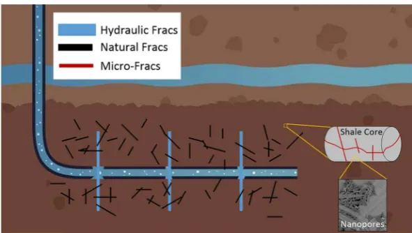
Fig 1 – Multi-scale natural of shale gas production 4
5
6
Fig 2 – Multi-scale shale gas storage and transport 7
In recent years, significant efforts have been made to model gas flow in unconventional reservoirs. 8
These methods can be categorized into analytical model, semi-analytical model and numerical 9
simulations. The analytical method dates back to 1970s, where the line-source fundamental solution is 10
derived for simple fracture geometry such as single bi-wing hydraulic fractures and pseudo-pressure is 11
applied to linearized the non-linear real gas equation (Gringarten et al, 1974, Cinco et al, 1978 and 12
Agarwal 1979). Recently, the analytical method is extended into semi-analytical method to consider 13
complex fracture networks and shale gas storage mechanism based on the boundary element method 14
(Zuo et al, 2016, Chen et al, 2015, 2016, 2017, 2018; Yang et al, 2016a, 2016b, 2017, Yu et al, 2016b, 15
2017 and Li et al, 2018). Although analytical-based method is fast and accurate, it is difficult to handle 16
4
shale gas flow problems (Houze et al, 2010 and Olorode et al, 2013). On the other hand, numerical 1
simulation has been proven to be is the most general and rigorous method to account for arbitrary 2
non-linear physics and fracture geometry for unconventional reservoirs (Olorode et al, 2013,2017 and 3
Cipolla et al, 2012). Highly coupled non-linear physics and treatment of multi-scale fractured system 4
are two key issues in shale gas flow simulation. Fully implicit scheme with Automatic Differentiation 5
(AD) is a robust and generic method to solve the highly coupled non-linear problem accurately and 6
efficiently (Zhou et al, 2011 and Krogstad et al, 2015). In terms of multi-scale fractured system, dual 7
continuum method (Warren and Root, 1963) and discrete fracture method (Karimi-fard et al, 2004, 8
Hoteit and Firoozabadi, 2005, Hajibeygi et al, 2011 and Moinfar et al, 2014) are generally used to model 9
highly connected fractures and long, disconnected hydraulic/natural fractures (Fig. 1), respectively. A 10
hierarchical method is also proposed by integrating continuum method and discrete fracture method for 11
multi-scale fractured system where the micro-fractures are upscaled into matrix permeability tensor and 12
hydraulic/natural fractures are modeled explicitly (Lee et al, 2001and Karimi-Fard et al, 2006). 13
Unstructured gridding with local grid refinement (LGR) is generally used to capture the irregular 14
fracture geometry and sharp pressure gradient near the fractures. However, it is are still challenging to 15
generate conforming mesh efficiently for complex fracture networks (Karimi-Fard, Durlofsky, 2016). 16
Recently, an embedded discrete fracture model is developed to resolve the complex gridding issue. 17
Using EDFM, the complex fractures are embedded in conventional matrix grids without conforming the 18
matrix grids with fracture plane, thus it is more efficient for complex fracture networks. In addition, it 19
can be easily integrated into well-established reservoir simulator without accessing the code (Xu, 2015 20
and Olorode et al, 2017). Table 1 shows the advantages and disadvantages of these method where 21
unstructured grid and EDFM are the two most promising methods for generic shale gas simulation with 22
multi-scale fractures. 23
Table 1. Comparison of shale gas flow simulation methods 24
Analytical Semi-analytical Structured grid Unstructured grid EDFM
Accuracy ++ ++ +++ +++ ++
Nonlinear mechanisms* + + +++ +++ +++
Rock heterogeneity + + +++ +++ +++
Fracture gridding +++ +++ + + +++
Preprocessing** efficiency +++ +++ +++ +++ ++
5
* Nonlinear gas transport & storage model, multi-phase flow, compositional flow
** 2D/3D geometry calculations, such plane-plane intersection, point-plane distance
*** linear algebra and Newton’s calculations
Flow and transport theory and models for unconventional reservoir is a rapid evolving area of 1
research, many of the existing and newly discovered phenomenon have not been completely understood. 2
Also, the effect of these mechanism on practical well performance is not clear. To the best of our 3
knowledge, almost all existing numerical models for shale gas reservoir are implemented in in-house 4
simulators or commercial simulators (Jiang and Younis, 2015, Cao et al, 2016, Xu et al, 2017, Wang et 5
al, 2017 and Akkutlu et al, 2018). Hence, it is necessary to develop a flexible and generic open-source 6
framework to fill this gap. 7
In this paper, a generic numerical model is developed to simulate shale gas flow in unconventional 8
reservoirs with multi-scaled fractures, which can be used to integrate any shale gas transport and 9
storage mechanism for unconventional reservoirs as well as the geomechanics effect for fracture 10
system. An efficient and flexible framework (OpenShale) is also developed using an open-source 11
reservoir simulation toolkit (MRST) and EDFM. OpenShale can handle deterministic hydraulic 12
fractures and stochastic natural fractures with arbitrary geometry and distribution. The framework is 13
firstly verified against a commercial simulator and an in-house reservoir simulator that employs 14
unstructured grid to simulate shale gas transport with non-planar hydraulic fracture, gas desorption, 15
gas slippage & diffusion. The advantages and limitation of EDFM for shale gas flow problem is also 16
discussed. Finally, field application of history matching and new geomechanics model evaluation are 17
studied. 18
2 Mathematical equations
19
Considering the isothermal single-component single-phase gas flow in 2D fractured porous media 20
with 1D fracture line without gravity effect. The general governing equation for shale gas flow in matrix 21
(m), considering storage (mad) and transport mechanisms (Fapp), can be expressed as follows:
22
, 0(1 ) ( i app i ) in
g ad g g w m
g
F k
m p q
t
(1)
23
Similarly, the governing equation for fracture (f), only considering transport mechanisms, can 24
6
( , 0 ) inapp i i
g g g w f
g
F k
p q
t
(2) 1Introducing inverse formation volume factor bg g / gsc (g bggsc), the above equation can 2
be rewritten as follows: 3
, 0
, 0
(1 )
( ) in
( ) in
app i i
g ad g g w m
gsc g
app i i
g g g w f
g
F k
b m b p b q
t
F k
b b p b q
t
(3)4
wheregis the mass density of gas, M/L3; g is the dynamic viscosity of natural gas, N.T/L2mad
5
is the accumulation term due to adsorption, M/L3; is the matrix porosity, dimensionless; k
0 is the
6
absolute Darcy permeability of the reservoir rock, L2.F
app,i is the i-th permeability correction factor
7
for a specific shale gas transport mechanism; qw is the volumetric sink/source term, M/L3/T. k0 is the
8
absolute Darcy permeability of the reservoir rock, L2.
9
2.1 Gas properties 10
Density: The pressure-dependent density of natural gas can be calculated by the real gas law: 11
( , )
g
pM Z p T RT
(4)
12
where M is the molecule weight of the natural gas, M/Mol; R is the Boltzmann constant, 8.314 13
ML2T-2/T/mole); T is the reservoir temperature, T;
14
The compressibility factor Z can be calculated using either implicit Peng-Robinson 15
equation-of-state (PR-EOS) equation or empirical explicit equation. Using the empirical equation, 16
the complex natural gas mixture can be considered as a single component with pseudo-temperature 17
and pseudo-pressure. Mahmoud (2014) developed an explicit empirical equation for natural gas 18
mixture as follows: 19
2.5 2 2.5 2
( , )=0.702 Tpr 5.524 Tpr (0.044 0.164 1.15)
pr pr pr pr
Z p T e p e p T T (5)
20
where the reduced-temperature and reduced-pressure can be expressed as Tpr T T/ c and 21
/
pr c
p p p , respectively. Tpc ands Ppc are the pseudo-critical pressure and pseudo-critical
22
temperature for the shale gas mixture, respectively. 23
7
estimated by solving a cubic function of PR-EOS as follows (Lira and Elliott, 2012): 1
3 2
2 1 0
2 3 2
0 1 2
2
2 2 0
( , ) ( ), ( , ) 3 2 , ( , ) 1
/ ( ) , / ( )
0.457235 0.0777961
,
c c
c c
Z a Z a Z a
a p T AB B B a p T A B B a p T B
A ap RT B bp RT
R T RT
a b
p p
(6)
2
In this paper, an analytical solution (see details in appendix B of Lira and Elliott, 2012) is used 3
for solving the cubic equation. For more complex natural gas mixture, it requires complex flash 4
calculation and belongs multi-component compositional simulation which will be investigated in our 5
future work. Fig. 3 shows an estimation of Z-factor for methane using Eq.5 and Eq. 6, respectively. 6
7
Fig. 3 Evaluated natural gas Z-factor for empirical and PR-EOS models with T=352 K, 8
Tc=191 K, pc=4.64 MPa, R=8.314 J/(K.mol)
9
10
Fig. 4 Evaluated natural gas viscosity using Lee Lee-Gonzalez-Eakin empirical correlation 11
with M=16.04 g/mol and T=633.6 Rankine 12
0 100 200 300
Pressure [Bar]
0.85 0.9 0.95
1 Gas Z-factor
Peng-Robinson
Empirical(Mahmoud, 2013)
0 100 200 300
Pressure [Bar]
0.012 0.014 0.016 0.018 0.02 0.022
8
Viscosity: The density-dependent viscosity of natural gas can be estimated by 1
Lee-Gonzalez-Eakin empirical correlation (Lee et al, 1966) as follows: 2
7
1.5
10 exp( ) (9.379 0.01607 ) 986.4
, 3.448 0.01009 , 2.447 0.2224 209.2 19.26
Y
g K X g
M T
K X M Y X
M T T
(7) 3
where the unit of M, T are g/mol and Rankine, respectively. Fig. 4 shows an estimation of 4
viscosity for methane using Eq.7. 5
Noted that although the usage of pseudo-pressure equation can eliminate the nonlinearity issue 6
introduced by pressure-dependent gas viscosity and compressibility (Eqs. 5-6), it leads lead to even 7
larger errors especially for tight shale reservoirs (Houze et al, 2010). Thus, in this paper, the real-gas 8
equation is used. 9
2.2 Transport and storage mechanism 10
Since rapid commercial development of unconventional tight reservoirs in recent years, many 11
researchers spend enormous effort to understand the transport and storage mechanism of shale gas in 12
such complex multi-scale systems (Figs. 1-2). Several key physical mechanisms (Yu et al, 2016; 13
Klinkenberg, 1941; Florence et al, 2007; Javadpour, 2007; Civan, 2010) can be summarized as in Table 14
2. 15
In the presented open-source code, OpenShale, any storage and transport mechanisms models can be 16
easily implemented via defining nonlinear gas storage function (mad) and permeability correction
17
function (Fapp). Demonstrative storage and transport models implemented in OpenShale this study are
18
shown as follows: 19
Table 2. Key transport and storage mechanism for shale gas flow 20
Mechanism Models Type Continuum
Adsorption Langmuir, BET S* Matrix
Slip flow & Diffusion Klinkenberg, Florence, Javadpour, Civan T* Matrix
Non-Darcy flow Darcy-Forchheimer T Fracture
*S-Storage mechanism, T-Transport mechanism
Adsorption: The gas molecules adsorbed in the pore wall of Kerogen in shale reservoir can be 21
modeled using monolayer Langmuir isotherm and multiple layer BET isotherm as follows (Yu et al, 22
9
Langmuir: L
ad s gsc
L pV m
p P
(8)
1
1 1
1 ( 1) BET:
1 1 ( 1) 1306.5485 , exp(7.7437 )
19.4362
n n
m r r r
ad s gsc n
r r r
r s
s
V Cp n p np
m
p C p Cp
p
p P
P T
(9)
2
whereVL is the Langmuir volume, L3/M. PL is the Langmuir pressure, M/L/T2. s is the density
3
of rock bulk matrix M/L3, V
L is the Langmuir volume (the maximum adsorption capacity at a given
4
temperature), L3/M. P
L is the Langmuir pressure (the pressure at which the adsorbed gas volume is
5
equal to VL/2), M/L/T2. Vm is the BET adsorption volume, L3/M. C is the BET adsorption constant,
6
dimensionless. n is the BET adsorption molecular layers, dimensionless. ps is the pseudo-saturation
7
pressure, M/L/T2. Noted that, the unit of P
s is MPa. Fig. 5 shows an estimation of adsorption
8
isotherm using Eq.8 and Eq. 9, respectively. 9
10
Fig. 5 Langmuir and BET isotherms curve with VL=0.0031 m3/kg and PL=7.89 MPa,
11
T=327.59 K, Ps=53.45 MPa, Vm=0.0015 m3/kg, C=24.56 and n=4.46
12
Slippage flow & Diffusion: Considering slippage and diffusion effect of shale gas flow in the 13
matrix, the apparent permeability in the low-pressure region around the fracture will be increased. In 14
the OpenShale, the Florence’s (2007) permeability correction factor (Fig. 4) is implemented as 15
follows: 16
4
(1 )(1 )
1 n
app n
n K
F K
K
(10)
17
A
d
so
rb
e
d
G
as
[m
3 /k
g
10
0
1 0.4 2
2.8284 2
128
tan (4 )
15 g n
g
n RT K
p M k
K
(11)
1
where Kn is the Knudsen number, dimensionless. is the rarefaction parameter, dimensionless. 2
Fig. 6 shows an estimation of gas slippage and diffusion permeability correction factor for methane
3
using Eqs. 10-11. 4
Non-Darcy Flow: In case of high Forchheimer number (Foc>0.11) in the hydraulic fractures, the
5
linear Darcy flow is no longer applicable (Zeng and Grigg, 2006). The permeability correction factor 6
(Barree and Conway, 2004) for Darcy-Forchheimer flow can be expressed as follows: 7
2 0
2
1 1 4
app
g g F
k
p
(12)
8
9
Fig. 6 – Permeability correction factor Fapp versus Knudesen number for all flow regions with
10
methane properties in Table 2, T=191 K, k0=1e-10 and =0.1
11
where is the empirical Forchheimer coefficient, for propped hydraulic fractures, which can be 12
evaluated as follows (Rubin, 2010): 13
9
15 1.021 0
1.485 10 3.2808
(k 10 )
(13)
14
2.3 Geomechanics effect 15
As shown in Fig. 2, shale reservoir has multi-scale fractures. The fracture conductivity will be 16
decreased with increasing of production time due to the proppant embedment and fracture closure 17
11
paper, three types of fractures are defined based on their various length scales, including hydraulic 1
fracture (half-length 50-100 meters, aperture 1mm), natural fracture (half-length 1-20 m, aperture 2
0.1mm), and micro-fracture (half-length < 1m, aperture <0.1 mm). A new geomechanics model is 3
proposed herein by considering closure of micro-fracture, unpropped natural fracture and propped 4
fractures. 5
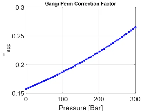
To consider the micro-fracture closure, Gangi’s (1978) empirical pressure-dependent 6
permeability reduction model can be applied as follows: 7
3
0 0
1 1
m
c B
app
P p
k k F k
P
(14)
8
Where B is the Biot’s constant, Pc is the confining overburden pressure, P1 is the effective
9
stress when micro-fracture completely closed. m is a constant related to surface roughness. Fig. 7 10
shows an estimation of Gangi permeability correction factor for methane using Eqs. 14. 11
12
Fig. 7 – Permeability correction factor Ffrac versus pore pressure with m=0.5, p1=180 MPa,
13
pc=38 MPa and =0.5
14
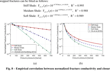
To consider the closure of hydraulic and natural fractures, Alramahi and Sundberg (2012) 15
performed experiment to measure the effect of closure pressure on propped fracture conductivity for 16
different shale samples from stiff shale to soft shale. An empirical model of normalized fracture 17
conductivity for propped fractures, Fcd,N, can be fitted as follows:
18
0.00011 0.0971 2 ,
0.00035 0.2396 2 ,
0.00064 0.4585 2 ,
Stiff Shale: F ( ) 10 , R 0.961
Meidum Shale: F ( ) 10 , R 0.996
Soft Shale: F ( ) 10 , R 0.987
cd N
cd N
cd N p
p p
(15)
19
0 100 200 300
Pressure [Bar]
0.15 0.2 0.25
12
Wu et al (2018) performed similar experiment to investigate the effect of closure pressure on 1
unpropped fracture conductivity. An empirical model of normalized fracture conductivity for 2
unpropped fractures can be fitted as follows: 3
0.793ln( ) 4.5618 2 ,
0.89ln( ) 5.0725 2 ,
1.041ln( ) 6.0216 2 ,
Stiff Shale: F ( ) 10 , R 0.995 Meidum Shale: F ( ) 10 , R 0.988 Soft Shale: F ( ) 10 , R 0.989
c c c cd N cd N cd N p p p (16) 4 5
(a) (b) 6
Fig. 8 – Empirical correlation between normalized fracture conductivity and closure 7
pressure for propped fractures (a) and unpropped fractures (b) 8
Where effective closure stress σc can be calculated by reservoir horizontal stress and in-situ
9
fracture pore pressure, c( )p h p. Plane direction of hydraulic fracture is normally orthogonal 10
to the minimum horizontal stress and it support by rigid proppant, while the plane of natural fracture 11
has stochastic orientation and lacking support from proppant. Thus, the closure stress for hydraulic 12
fracture and natural fracture can be expressed as follows: 13 min min max HydraulicFrac: NaturalFrac: 2 HF h h h NF p p
(17)
14
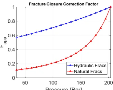
The empirical correlation between fracture conductivity and closure pressure are shown in Fig. 15
8. In the OpenShale, the fracture permeability can be reduced by a dynamic permeability correction 16
factor as follows: 17 0 0 0 ( ) ( ) cd f app cd F p
k k F k
F p
(18)
18
Based on proposed empirical correlation model in Eqs. 15-16, a typical permeability correction 19
factors for fracture closure can be shown as follows (Fig. 9): 20
0 100 200 300 400 500 600 700
Closure pressure [barsa]
10-6 10-4 10-2 100 Stiff Shale Median Shale Soft Shale
Alramahi and Sundberg (2012)
0 100 200 300 400 500 600 700
Closure pressure [barsa]
10-4 10-3 10-2 10-1
100 Stiff Shale
13
1
Fig 9 – Permeability correction factor Ffrac for hydraulic fractures and natural fractures
2
with po = 20.34 MPa and pwf = 34.5 MPahmin= 29 MPa andhmax= 34 MPa
3
3 Numerical Model
4
In this paper, a new shale gas simulation framework, OpenShale , is developed using the automatic 5
differentiation module (ad-core, ad-props), black-oil module (ad-blackoil) and hierarchical fracture 6
model (hfm) module in open-source MATLAB Reservoir Simulation Toolbox (Lie, 2012). Two-point 7
flux approximated finite volume method (TPFA-FVM) is applied for discretizing the governing 8
equations (Eq. 3). Time discretization is implemented using a fully implicit first-order backward 9
scheme, where the Jacobian matrix of the nonlinear system is calculated by Automatic Differentiation. 10
All nonlinear functions for shale gas transport and storage mechanisms as well as geomechanics effect 11
are defined as separate function. For multi-scale fracture system, the larger fracture, such as the 12
hydraulic fracture and natural fracture are explicitly modeled using EDFM. The micro-fractures are 13
assumed highly connected and thus upscaled into the matrix permeability. 14
3.1 Numerical discretization 15
The discretized governing equation of Eq. 3 can be expressed as follows: 16
1
1
1 ,
1 1
1
1 1 1 1
(1 ) 1
( ) ( ) ( ) ( )
( )
( ) ( )
( )
( ) ( ) ( ) ( ) 0
n n n n
g g ad ad
gsc
n app i
n i n
g n
g
n n n n
g w g f m
V V
b p b p m p m p
t t
F p
b p T p
p
Vb p q p Vb p p
div grad (19)
17
14
1
1 ,
1 1
1
1 1 1 1
( ) ( )
( )
( ) ( )
( )
( ) ( ) ( ) ( ) 0
n n
g g
n app i
n i n
g n
g
n n n n
g w g m f
V
b p b p
t
F p
b p T p
p
Vb p q p Vb p p
div grad (20)
1
where V is the bulk volume of a grid cell. f m m f / is the flow coupling term between fracture 2
and matrix. To simplify the implementation of governing equations (Eqs. 18-19), three discrete 3
domain delta functions for matrix (m), hydraulic fractures (HF) and natural fractures (NF) can 4
be defined as follows: 5
1 1 1
( ) , ( ) , ( )
0 0 0
m HF NF
m HF NF
m HF NF
x x x
x x x
x x x
(21)
6
A generic numerical model for fractured reservoir considering shale gas transport and storage 7
mechanism can be expressed as follows: 8
1
1
1
/ , ,
1 1
1
1 1 1 1
/
(1 ) 1
( ) ( ) ( ) ( )
1 ( )
( ) ( )
( )
( ) ( ) ( ) ( ) 0
ijk n n ijk n n
g g m ad ad
gsc
n HF NF i app i
n i n
g n
g
n n n n
ijk g w ijk g f m m f
V V
b p b p m p m p
t t
F p
b p T p
p
V b p q p V b p p
div grad (22)
9
Assuming vertical well fully penetrate the reservoir thickness, a semi-analytical well model 10
(Peaceman, 1983) for a vertical well can be expressed as follows: 11
/ ( )
w g bh
q WI p p (23)
12
where pbh is the bottom hole pressure of a wellbore, M/L/T2. WI is the wellbore flow index.
13
The solution matrix from Eqs. 21 can be expressed as follows: 14
# # MatrixEles, # # FractureEles, # #Eles has well
mm mf mw m m
fm ff fw f f
wm wf ww w w
m f w
A A A p Q
A A A p Q
A A A p Q
p p p
(24)
15
Noted that the shale gas viscosity, density and permeability corrections terms are all depends on 1
solution variables. To solve non-linear system of Eq. 23, the residual form of Newton’s iterations can 2
be expressed as follows: 3
1 1
( )(i i i) d ( )(i i i) ( )i
d
R
J x x x x x x R x
x (25)
4
The Jacobian matrix J is calculated by automatic differentiation in MRST. 5
3.2 EDFM 6
7
Fig. 10 – Grid system in EDFM for matrix, natural fracture and hydraulic fracture 8
As shown in Fig. 10, EDFM adopted the concept of dual-continuum fracture modeling method,
9
the flow coupling term f m m f / is introduced to couple the solution among matrix and fractures. 10
Thus, the matrix grid is not necessary conforming with the fracture plane. As shown in Fig. 11, there 11
are three kinds of non-neighbor connection (NNC) in EDFM formulation: 1) fracture-matrix 12
connectivity, 2) fracture-fracture connectivity and 3) fracture-well connectivity. The general NNC 13
model can be expressed as follows (Xu, 2015): 14
1 1
( )
NNC NNC n n
f m f m f m
NNC NNC
f m m f
T p p
(26)
15
16
Fig. 11 – Unit EDFM NNCs of 1) fracture-matrix (i-k pair) connectivity 2) fracture-fracture
17
(j-k pair) connectivity and 3) fracture-wellbore (well-k pair) connectivity
18
Fracture-matrix NNC: The fracture-matrix transmissibility (Tf-m) can be expressed as follows:
19
i
k
i+1
i-1
Unit EDFM System
16
0,
,
NNC ik ik
ik
g ik ik
k A
T
d
(27)
1
where Ai,k is the intersection area fraction between a fracture plane and a gridblock. For 2D grid,
2
the area is the product of intersected fracture cell length within the matrix cell and uniform formation 3
thickness, DZ. Noted that the harmonic average and upwind scheme are used for the permeability 4
and viscosity, respectively. d i k, is the average normal distance between matrix cell and fracture 5
plane, which can be calculated as follows: 6
ik ik
i d dv d
V
(28)7
For 2D structured grid, an analytical solution is available for the average normal distance (see 8
Tene et al, 2016). 9
Fracture-fracture NNC: the star-delta transformation can be used to calculate the 10
transmissibility between intersected fractures as follows (Hajibeygi et al, 2011): 11
ints
, 0,
, ,
1
,
0.5
j k f m
NNC m
jk N m
f m g m m
m
t t A k
T t
h
t
(29)12
where Af is the cross-section area of a fracture plane, for 2D cell, which can be calculated by
13
product of fracture aperture, wf, and formation thickness. hf is the fracture cell length.
14
Fracture-well NNC: If a well intersected with a fracture cell, the effective wellbore index (WI) 15
and equivalent radius (re) can be expressed as follows (Xu, 2015):
16
2 2
2
, 0.14
ln( / ) f f
f e f
e w
k w
WI r h DZ
r r s
(30)
17
where s is the skin factor, dimensionless, which will be used as a correction factor to correct the 18
error introduced by EDFM when model low-permeability fractures. DZ is the formation thickness, L. 19
4 Verification
20
To verify the presented general shale gas model (Eq. 21), two numerical simulations are performed 21
against a commercial simulator (CMG, 2015) and an in-house simulator with unstructured mesh (Jiang 22
and Younis, 2015). The base model and simulation parameters for all cases as shown in Table 3: 23
Table 3—Base model and simulation parameters for all cases 24
17
Rock density kg/m3 2500
Molecular weight, CH4 kg/mol 0.01604
Critical pressure, CH4 MPa 4.60
Critical temperature, CH4 K 190.6
Acentric factor, CH4 - 0.01142
Well radius m 0.1
1
4.1 Case 1 – Verification against commercial simulator 2
OpenShale is firstly verified in a simple methane production case against a commercial 3
simulator (CMG) with a single vertical hydraulic fracture (Fig. 12). By changing the hydraulic 4
conductivity, grid schemes and natural fractures, three subcases (Case1a, Case1b and Case1c) are 5
investigated. The accuracy of OpenShale with explicit fracture modeling (EFM) and EDFM are 6
systematically studied. In this simulation, only Langmuir adsorption (Eq. 8) is considered. All fluid 7
properties and simulation parameters are the same with the commercial simulator. The 8
compressibility factor Z and natural gas viscosity are directly interpolated from the properties table 9
of the commercial simulator. Detailed simulation properties are shown in Table 4. 10
Table 4. Key reservoir and simulation parameters of Case 1 11
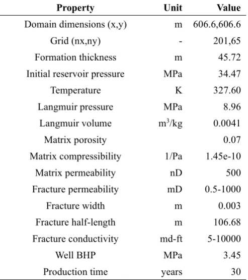
Property Unit Value
Domain dimensions (x,y) m 606.6,606.6
Grid (nx,ny) - 201,65
Formation thickness m 45.72 Initial reservoir pressure MPa 34.47
Temperature K 327.60
Langmuir pressure MPa 8.96
Langmuir volume m3/kg 0.0041
Matrix porosity 0.07
Matrix compressibility 1/Pa 1.45e-10
Matrix permeability nD 500
Fracture permeability mD 0.5-1000
Fracture width m 0.003
Fracture half-length m 106.68 Fracture conductivity md-ft 5-10000
Well BHP MPa 3.45
18
1
(a) (b) 2
Fig. 12 Fracture map (a) and pressure contour after 30 years production (b) of Case 1a 3
and Case1b 4
Case1a: In the first subcase, three fracture conductivities (10000 md-ft, 50 md-ft, 5 md-ft) are 5
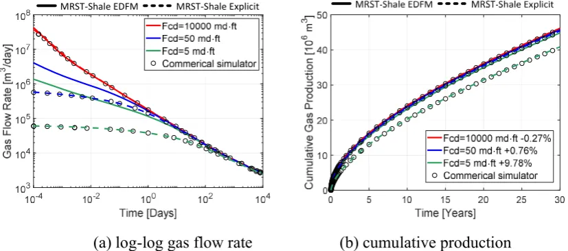
used to verify the accuracy of OpenShale with EFM and EDFM. Fig. 13 shows a good agreement of
6
both gas flow rate and cumulative production between OpenShale and commercial simulator. Results 7
show that OpenShale with EFM (dash line) always gives consistent results against commercial 8
simulator. But OpenShale with EDFM (solid) has significant error (up to 10.92%) when fracture 9
conductivity is low (5 md-ft). Fig. 12a shows that OpenShale EDFM only converges to reference 10
solution under infinite fracture conductivity (10000 md-ft). This is observation matches Tene 11
(2017)’s conclusion that EDFM can not handle the fracture with low permeability. 12
13
(a) log-log gas flow rate (b) cumulative production 14
Fig. 13 Comparison of gas flow rate (a) and cumulative production (b) for Case 1a 15
between OpenShale EDFM (solid line), OpenShale EFM (dash line) and a commercial 16
19
simulator (dots) with respect to fracture conductivities of 5 md-ft (green lines), 50 md-ft (blue 1
lines) and 10000 md-ft (red lines) 2
Case1b: For unconventional tight reservoir, LGR is usually required to capture the transient 3
flow behavior and sharp pressure gradient near the hydraulic fractures. In the second subcase, the 4
effect of grid schemes on accuracy of OpenShale with EFM and EDFM are investigated. In this case, 5
the fracture conductivity is set as 10000 md-ft to eliminate the EDFM error mentioned in Case1a. All 6
other parameter is the same with Case1a. As shown in Fig. 14, three grid schemes are investigated, 7
where LGR scheme with logarithmic refinement that is solved by OpenShale EFM; EDFM scheme is 8
the standard EDFM grid scheme (Xu et al, 2017 and Tene et al, 2017) with uniform grid that is 9
solved by EDFM; EDFM+LGR scheme is the same grid scheme as LGR scheme that an additional 10
EDFM fracture cell is added and that is solved by EDFM. Noted that all grid scheme has the same 11
grid dimension (nx,ny) of 499x61. 12
13
Fig. 14 EFM and EDFM Grid schemes for Case1b, fracture cell is shown 10 times larger 14
than the real size, where logarithmic refinement and uniform used in LGR and EDFM scheme, 15
respectively 16
Figs. 15-16 shows a good agreement of gas flow rate and cumulative production between
17
OpenShale and commercial simulator with respect to high fracture conductivity and low fracture 18
conductivity. OpenShale with EFM again gives consistent results against commercial simulator for 19
all grid schemes. However, the standard EDFM grid scheme can introduce an error of 3.31% for high 20
fracture conductivity and 1.11% for low fracture conductivity. The error is measured by the 21
20
benchmark case demonstrates that EDFM cannot capture transient flow behavior and sharp pressure 1
gradient near the hydraulic fracture without helping of LGR. 2
3
(a) log-log gas flow rate (b) cumulative production 4
Fig. 15 Comparison of gas flow rate (a) and cumulative production (b) for Case 1b with 5
high fracture conductivity of 10000 md-ft between OpenShale and a commercial simulator 6
(dots) 7
8
(a) log-log gas flow rate (b) cumulative production 9
Fig. 16 Comparison of gas flow rate (a) and cumulative production (b) for Case 1b with 10
low fracture conductivity of 5 md-ft between OpenShale and a commercial simulator (dots) 11
Case1c: As mentioned in Case1a and Case1b, EDFM cannot handle low-permeability fracture 12
and hydraulic fractures with sharp pressure gradient. But modeling of natural fracture network is 13
quite challenge for the EFM. In this subcase, the effect of different grid schemes of natural fractures 14
on accuracy for OpenShale with EDFM is also investigated. As shown in Fig. 17, six natural 15
fractures with the same length of 116.74 m are added based on the Case1a. The well performance of 16
21
hydraulic fracture and natural fractures are set as 10000 md-ft and 5 md-ft, respectively. All other 1
parameters are the same with Table 3. 2
3
Fig. 17 Grid schemes of Case 1c, number of grids are shown 20 times coarser than the real 4
scheme. LGR scheme with LGR for natural fractures, EDFM scheme without LGR for natural 5
fractures 6
Fig. 18 demonstrates that OpenShale with EDFM can lead to a significant error (up to 16.99%)
7
for the case where low-permeability natural fractures connected with high-permeability hydraulic 8
fractures. Also, EDFM without LGR for natural fractures tends to underestimate the well 9
performance (error of 3.4% for six natural fractures). This benchmark case indicates that EDFM is 10
not capable to accurately model well performance of shale gas flow in ultra-tight reservoir due to the 11
errors introduced by low-permeability fracture and grid refinement. 12
13
(a) log-log gas flow rate (b) normalized cumulative production 14
Fig. 18 Comparison of gas flow rate (a) and normalized cumulative production by NFs (b) 15
22
In sum, this case study shows that OpenShale with EFM always give consistence results against 1
commercial simulator, while OpenShale with EDFM only converge to the reference solution at 2
infinite fracture conductivity (Case1a). Also, OpenShale with EDFM cannot handle low-permeability 3
fracture (Case1b) and cannot capture transient behavior and sharp gradient without LGR (Case1c). 4
OpenShale with EDFM can model complex and irregular natural fractures accurately and efficiently. 5
Thus, in the following simulations, an empirical skin-factor and uniform grid refinement are adopted 6
to relieve the limitations of EDFM. More advanced projected EDFM (Tene et al, 2017) and 7
adaptively grid refinement will be implemented in our future work. 8
4.2 Case 2 – Verification against in-house simulator 9
OpenShale is further verified against an in-house simulator (Jiang and Younis, 2015) by 10
considering more comprehensive state-of-art transport mechanisms and fracture geometries. For the 11
reference solution, it used fully unstructured mesh with LGR to capture the complex fracture 12
geometries as well as the sharp pressure gradient near the fracture. In this case, the gas rate solution 13
of two sub-case are investigated. In the first sub-case (Case2a), the well performance with and 14
without storage (Eq. 8) and transport mechanism (Eq. 10) is considered. In the second sub-case 15
(Case2b), the irregular fracture geometry is considered. The fracture map of Case2a is shown in Fig. 16
19. Detailed simulation parameters for Case 2 are elaborated in Table 4. 17
18
Fig. 19 Fracture map and EDFM grid of Case 2 19
Table 4. Key reservoir and simulation parameters of Case 2 20
Property Unit Value
Domain dimensions (x,y) m 200,140 Formation thickness, m 10 Initial reservoir pressure MPa 16
Temperature K 343.15
Langmuir pressure MPa 4
0 50 100 150 200 0
20 40 60 80 100 120
140 Fracture Map
(50,40) (50,100)
23
Langmuir volume m3/kg 0.018
Matrix porosity 0.1
Matrix compressibility 1/Pa 1.0e-9
Fracture porosity 1.0
Matrix permeability nD 100 Fracture permeability D 1
Fracture width m 1e-3
Well BHP MPa 4
Correction skin factor - 43 Production time days 10000
Other parameters are the same as in Table 2
Fig. 20 shows pressure contour after 2500 days of production for Case 2 with and without
1
transport mechanisms. It can be observed that the sub-case with full mechanism has better pressure 2
depletion (dark blue region) than one without any mechanism. Fig. 21 shows a good agreement 3
between gas flow rate between OpenShale and an in-house simulator, where demonstrates that the 4
both adsorption and gas slippage and diffusion effect increase the gas production significantly. In 5
tight unconventional reservoirs, smaller pore-throat and lower bottom-hole pressure can lead to 6
higher production due to gas slippage flow and releasing adsorbed gas. 7
8
Fig. 20 Pressure contour with and without full shale gas transport mechanism @ 2500 9
24
1
(a) log-log gas flow rate (b) cumulative production 2
Fig. 21 Comparison of gas flow rate (a) and cumulative production (b) for Case 2a 3
between OpenShale and an in-house simulator 4
5 Application
5
In the previous sections, OpenShale shows it capability to handle arbitrary transport and storage 6
mechanism and fracture geometries. To further illustrate the applicability of OpenShale in practical 7
problems, two case studies of OpenShale in realistic unconventional reservoirs with complex fracture 8
network are presented. 9
5.1Case 3: History matching and production forecast
10
To further verify the applicability of the OpenShale. A history matching with field production 11
data on a Barnett shale has performed. The field production and simulation data are adopted from 12
literature (Cao, Liu and Leong, 2016; Yu and Kamy Sepehrnoori, 2014). The detailed reservoir and 13
fluid parameters are shown as in Fig. 22 and Table 5. 14
15
10-4 10-2 100 102 104 Time [Days]
101 102 103 104 105
Full Mechanism Adsorption only Slippage & diffusion only No Mechanism Jiang and Younis, 2015
0 5 10 15 20 25
Time [Years] 0
1 2 3 4 5
25
1
Fig. 22 Fracture map and EDFM LGR grid with 28 planar hydraulic fractures of Case 3 2
Table 5. Key reservoir and simulation parameters of Barnett shale for Case 3 (Cao, 2016) 3
Property Unit Value
Domain dimensions (x,y) m 1200,300
Depth m 5463
Formation thickness, m 90 Initial reservoir pressure MPa 20.34
Temperature K 352
Rock density kg/m3 2500
Langmuir pressure MPa 4.47 Langmuir volume m3/kg 0.00272
Matrix porosity 0.03
Matrix compressibility 1/Pa 1.5e-10 Fracture compressibility 1/Pa 1.0e-8 Matrix permeability nD 200 Fracture permeability mD 100
Fracture width m 0.003
Fracture spacing m 30.5
Fracture half-length m 47.2 Fracture conductivity md-ft 1
Well BHP MPa 3.69
Correction skin factor - 19 Production time days 1600
Other parameters are the same as in Table 2
In this simulation, a rectangle reservoir with dimension of 1100 × 290 × 90 m was discretized 4
by 148 × 39 × 1 grids. 28 stages hydraulic fractures in the center of domain with the half-length of 5
47.2 m and the fracture spacing of 30.5 m. The fractures are assumed have constant aperture of 0.003 6
m and permeability of 100 md. Only shale gas storage mechanism of Langmuir adsorption (Eq. 8) is 7
considered. Fig. 23 shows the pressure contour at different production time (400 days and 1600 8
26
shows good agreements with the field production data. Based on matched simulation parameters, the 1
production forecast can be easily performed as in Fig. 21. 2
3
Figure 23 Pressure contour after 1600 days production for Barnett shale reservoir (Case 3) 4
5
(a) (b) 6
Fig. 24 History matching (a) and production forecast (b) of a Barnett shale well (Case 3) 7
5.2Case 4: New model evaluation
8
To illustrate the capability of modular design and rapid prototyping of OpenShale, a new shale 9
gas model considering geomechanics effect (Eqs. 15-17) for multi-scale fractured network is 10
implemented and evaluated using OpenShale. In this section, the influence of multi-scale fracture 11
network and geomechanics effect on shale gas production performance will be investigated. 12
13
Fig. 25 Fracture map with 28 non-planar hydraulic fractures and 248 natural fractures of 14
Case 4 15
100 101 102 103 104
Time [Days]
104 105 106
MRST-Shale Field Data
0 5 10 15 20 25 30
Time [Year]
0 0.5 1 1.5
2 105
27
In this case, all the simulation parameters are the same with Case 3 of Barnett shale reservoir. 1
The total length of non-planar hydraulic fractures (blue lines in Fig. 25) is the same as planar 2
fractures used in Case 3 (blue lines in Fig. 14). Natural fractures are stochastically generated by an 3
open-source fracture generator ADFNE (Alghalandis, 2017). The geomechanics parameters for shale 4
reservoir are assumed (Wasaki and Akkutlu, 2015) as follows (Table 5): 5
Table 5. Geomechanics parameters of Barnet shale for Case 4 6
Property Unit Value
Biot constant, - 0.5
Overburden confining stress, pc MPa 38
Maximum horizontal stress, shmax MPa 34
Minimum horizontal stress, shmin MPa 29
Maximum closure stress for micro-fracture, p1 MPa 180
Gangi exponential constant, m - 0.5 Natural fractures permeability md 10
Other parameters are the same as in Tables 2-3
7
(a) Non-planar hydraulic fracture (Same total fracture length with Case 3) 8
9
10
(b) Non-planar hydraulic fracture + natural fractures 11
Fig. 26 Pressure contour at the 3.75 years for Barnett shale reservoir with Non-planar fracture 12
28
1
(a) (b) 2
Fig. 27 Comparison of gas flow rate (a) and cumulative production (b) between Planar, 3
Non-planar and Non-planar & natural fractures cases 4
Firstly, the effect of complex fracture network on well performance is studied. Fig26 shows the 5
pressure contour for the non-planar fractures with and without the natural fractures. Obviously, the 6
case of natural fractures has larger and better stimulated reservoir volume (SRV). Thus, as shown in 7
Fig. 27, the cumulative gas production of non-planar case with natural fracture has much higher
8
value (14.56% improvements) than the planar case in the Case 3. While in the case of same total 9
length, the non-planar fracture geometries will slightly degenerate the well performance (-5.69% 10
reduction). 11
12
Non-planar hydraulic fracture + natural fractures + geomechanics effect 13
Fig. 28 Pressure contour at 3.75 years for Barnett shale reservoir with planar hydraulic 14
fractures case and realistic case 15
The influence of geomechanics effect with fracture closure on well performance is further 16
investigated by implementing Eqs. 15-17. Fig. 28 shows the pressure contour at the 3.75 years for 17
the planar case (Fig. 20a) and realistic case (Fig. 20b) with non-planar hydraulic fracture, natural 18
fractures and geomechanics effect. As shown in Fig. 29, at the earlier production period, even 19
realistic case has lower production than simple planar case due to geomechanics effect. But in the 20
10-2 100 102 104
Time [Days]
103 104 105 106
G
a
s
F
lo
w
R
a
te
[m
3 /d
a
y]
29
later production time, the contribution of natural fractures makes identical well performance between 1
realistic case and simple planar case. Thus, the modeling of natural fractures and geomechanics 2
effect is important for long-term production evaluation. 3
4
(a) (b) 5
Fig. 29 Comparison of gas flow rate (a) and cumulative production (b) between planar 6
hydraulic fracture case and realistic case with non-planar, natural fractures and geomechanics 7
effect 8
6 Conclusion
9
In this work, A generic numerical model and an open-source framework OpenShale are 10
developed for shale gas simulation with state-of-art flow and storage mechanisms. It is verified 11
against commercial and in-house reservoir simulators. The limitation of EDFM are also investigated 12
quantality. Also, a field application of history matching and new model evaluation of geomechanics 13
effect are successful performed. Several conclusions can be drawn as follows: 14
(1) A generic shale gas numerical model is developed which can be used to model any state-of-art 15
storage and transport mechanisms, including gas adsorption, gas slippage & diffusion, 16
non-Darcy flow as well as geomechanics effect by considering complex multi-scale fracture 17
geometries. 18
(2) A general and open-source framework, OpenShale is developed and verified. With the help of 19
the EDFM, Automatic Differentiation, and object-designed framework of OpenShale, one can 20
easily use and extend OpenShale to simulate practical shale gas problem with arbitrary fracture 21
geometries and new storage and transport mechanisms. 22
(3) EDFM can efficiently and accurately model irregular fracture geometry and complex fracture 23
10-2 100 102 104
Time [Days]
103
104 105 106
Planar
Non-planar+NFs+Geomechs Field Data
0 5 10 15 20 25 30
Time [Years]
0 50 100 150
C
u
m
u
la
tiv
e
G
a
s
P
ro
d
u
ct
io
n
[1
0
6 m 3]
Planar
30
networks. However, it cannot accurately model low-permeability fracture (error of 12.22%) and 1
hydraulic fractures without help of LGR where have strong transient behavior and sharp 2
gradient (error of 2.84%). Thus, projected EDFM and adaptively grid refinement will be 3
implemented and tested in our future work. 4
(4) Shale gas transport and storage mechanisms, such as gas desorption and gas slippage &diffusion 5
flow gas, are the most significant impact on well performance, follow by natural fractures, 6
geomechanics effect and fracture geometry. 7
(5) OpenShale is capable of serving as an efficient, flexible research tool to evaluate new models 8
with arbitrary non-linearity and fracture complexity. It can serve as a bridge between mechanism 9
study and field scale engineering application. 10
11
Nomenclature 12
g = mass density of natural gas, kg/m3
13
= absolute rock porosity, dimensionless 14
m = matrix domain 15
f = fracture domain 16
mad = storage mechanism term, kg/m3
17
Fapp = transport mechanism term, dimensionless
18
k0 = absolute Darcy rock permeability, m2
19
g = viscosity of natural gas, Pa∙s
20
p = pore pressure, Pa 21
qw = volumetric sink/source term, m3/day
22
bg = inverse formation volume factor, dimensionless
23
M = molecular weight of natural gas, kg/mol 24
Z = compressibility factor of natural gas, dimensionless 25
R = ideal gas constant, 8.314 J/(mol∙K) 26
T = reservoir temperature, K 27
Tpr = pseudo-temperature for natural gas, dimensionless
28
Tc = critical-temperature for natural gas, K
29
ppr = pseudo-pressure for natural gas, dimensionless
30
pc = critical-pressure for natural gas, Pa
31
a0,1,2 = constants for Peng-Robinson equation of state, dimensionless
32
a,b = constants for Peng-Robinson equation of state, dimensionless 33
A,B = constants for Peng-Robinson equation of state, dimensionless 34
K,X,Y= constants for Lee-Conzalez-Eakin natural gas viscosity, dimensionless 35
s = mass density of bulk matrix, kg/m3
36
gsc = mass density of natural gas at the standard condition, kg/m3
37
VL = Langmuir volume, m3/kg
31
PL = Langmuir pressure, Pa
1
Vm = BET volume, m3/kg
2
Ps = BET pseudo-saturation pressure, Pa
3
pr = psdueo-pressure for BET isotherm, dimensionless
4
C = constant for BET isotherm, dimensionless 5
n = constant for BET isotherm, dimensionless 6
= rarefaction coefficient for gas slippage flow, dimensionless 7
Kn = Knudsen number, dimensionless
8
= Darcy-Forchheimer coefficient, dimensionless 9
B = Biot’s coefficient, dimensionless
10
Pc = reservoir confining overburden pressure, Pa
11
P1 = reservoir effective stress when micro-fracture completely closed, Pa
12
m = constant for the Gangi’s model, Pa 13
Fcd = fracture conductivity, md∙ft
14
p0 = initial reservoir pressure, m
15
= effective fracture closure stress, Pa 16
hf = effective closure stress for hydraulic fracture, Pa
17
nf = effective closure stress for natural fracture, Pa
18
h = reservoir horizontal principle stress, Pa
19
hmin= minimum reservoir horizontal principle stress, Pa
20
hmax= maximum reservoir horizontal principle stress, Pa
21
kf = absolute Darcy permeability of fracture, m2
22
wf = fracture width, m
23
V = bulk volume of a grid cell, m 24
= discrete domain delta function, dimensionless 25
∆t = solution time-step, day 26
f-m = mass coupling term for matrix, dimensionless
27
m-f = mass coupling term for fracture, dimensionless
28
pbh = wellbore bottom hole pressure, Pa
29
k11 = absolute Darcy rock permeability in x-direction, m2
30
k22 = absolute Darcy rock permeability in y-direction, m2
31
re = equivalent radius for wellbore model, m
32
rw = wellbore radius, m
33
s = wellbore skin factor, dimensionless 34
∆x = grid cell size in x-direction, m 35
∆y = grid cell size in y-direction, m 36
∆z = grid cell size in z-direction, m 37
WI = wellbore index, dimensionless 38
x = Unknown vector, - 39
J = Jacobian matrix, - 40
R = Residual vector, - 41
WI = wellbore index, dimensionless 42
pf = pore pressure at the fracture domain, Pa
43
pm = pore pressure at matrix domain, Pa
32
T = transmissibility, dimensionless 1
A = intersection area among fracture and matrix, m2
2
d = average normal distance among fracture and matrix, m 3
hf = length of a fracture cell, m
4
t = fracture transmissibility for fracture-fracture NNC, dimensionless 5
6
Subscripts: 7
NF = natural fracture 8
HF = hydraulic fracture 9
m = matrix 10
f = fracture 11
g = gas 12
w = well 13
14
References 15
Akkutlu, I.Y., Efendiev, Y., Vasilyeva, M. and Wang, Y., 2018. Multiscale model reduction for 16
shale gas transport in poroelastic fractured media. Journal of Computational Physics, 353, 17
pp.356-376. 18
Akkutlu IY, Fathi E. Multi-scale gas transport in shales with local kerogen heterogeneities. SPE 19
J. 2012;17(4):1002–1011. 20
Alghalandis, Y.F., 2017. ADFNE: Open source software for discrete fracture network 21
engineering, two and three dimensional applications. Computers & Geosciences, 102, pp.1-11. 22
Alramahi, B. and Sundberg, M.I., 2012, January. Proppant embedment and conductivity of 23
hydraulic fractures in shales. In 46th US Rock Mechanics/Geomechanics Symposium. American 24
Rock Mechanics Association. 25
Agarwal, R.G., 1979, January. " Real Gas Pseudo-Time"-A New Function For Pressure Buildup 26
Analysis Of MHF Gas Wells. In SPE Annual Technical Conference and Exhibition. Society of 27
Petroleum Engineers. 28
Bowker, K.A., 2007. Barnett shale gas production, Fort Worth Basin: Issues and discussion. 29
AAPG bulletin, 91(4), pp.523-533. 30
Cipolla, C.L., Lolon, E.P., Erdle, J.C. and Rubin, B., 2010. Reservoir modeling in shale-gas 31
reservoirs. SPE reservoir evaluation & engineering, 13(04), pp.638-653. 32
Cao, P., Liu, J. and Leong, Y.K., 2016. A fully coupled multiscale shale deformation-gas 33
transport model for the evaluation of shale gas extraction. Fuel, 178, pp.103-117. 34
Civan F. Effective correlation of apparent gas permeability in tight porous media. Transp Porous 35
Media. 2010;82(2):375–384. 36
Chen, Z., Liao, X., Zhao, X., Dou, X. and Zhu, L., 2015. Performance of horizontal wells with 37
fracture networks in shale gas formation. Journal of Petroleum Science and Engineering, 133, 38
pp.646-664. 39
Chen, Z., Liao, X., Zhao, X., Dou, X. and Zhu, L., 2016. A semi-analytical mathematical model 40
for transient pressure behavior of multiple fractured vertical well in coal reservoirs incorporating 41
with diffusion, adsorption, and stress-sensitivity. Journal of Natural Gas Science and 42
33
Chen, Z., Liao, X., Sepehrnoori, K. and Yu, W., 2018. A Semianalytical Model for 1
Pressure-Transient Analysis of Fractured Wells in Unconventional Plays With Arbitrarily 2
Distributed Discrete Fractures. SPE Journal. 3
Chen Z, Liao X, Zhao X, Lyu S, Zhu L. A comprehensive productivity equation for multiple 4
fractured vertical wells with non-linear effects under steady-state flow. J Pet Sci Eng. 2017; 5
149:9–24. 6
Civan F, Rai CS, Sondergeld CH. Shale-gas permeability and diffusivity inferred by improved 7
formulation of relevant retention and transport mechanisms. Transp Porous Media. 8
2011;86(3):925–944. 9
Cinco, L., Samaniego, V. and Dominguez, A., 1978. Transient pressure behavior for a well with 10
a finite-conductivity vertical fracture. Society of Petroleum Engineers Journal, 18(04), 11
pp.253-264. 12
Elliott, J.R. and Lira, C.T., 2011. Introductory chemical engineering thermodynamics (Vol. 184). 13
Upper Saddle River, NJ: Prentice Hall PTR. 14
Florence, F.A., Rushing, J., Newsham, K.E. and Blasingame, T.A., 2007, January. Improved 15
permeability prediction relations for low permeability sands. In Rocky Mountain Oil & Gas 16
Technology Symposium. Society of Petroleum Engineers. 17
Hoteit, H. and Firoozabadi, A., 2005. Multicomponent fluid flow by discontinuous Galerkin and 18
mixed methods in unfractured and fractured media. Water Resources Research, 41(11). 19
Houze, O., Tauzin, E., Artus, V. and Larsen, L., 2010. The Analysis of Dynamic Data in Shale 20
Gas Reservoirs–Part 1. company report, Kappa engineering, Houston, Texas, USA. 21
Gringarten, A.C., Ramey Jr, H.J. and Raghavan, R., 1974. Unsteady-state pressure distributions 22
created by a well with a single infinite-conductivity vertical fracture. Society of Petroleum 23
Engineers Journal, 14(04), pp.347-360. 24
Karimi-Fard, M., Durlofsky, L.J., Aziz, K., 2004. An efficient discrete-fracture model applicable 25
for general purpose reservoir simulators. SPE J. 9 (2), 227e236. 26
Karimi-Fard, M., Gong, B. and Durlofsky, L.J., 2006. Generation of coarse‐scale continuum 27
flow models from detailed fracture characterizations. Water resources research, 42(10). 28
Karimi-Fard, M. and Durlofsky, L.J., 2016. A general gridding, discretization, and coarsening 29
methodology for modeling flow in porous formations with discrete geological features. 30
Advances in water resources, 96, pp.354-372. 31
Krogstad, S., Lie, K.A., Møyner, O., Nilsen, H.M., Raynaud, X. and Skaflestad, B., 2015, 32
February. MRST-AD–an open-source framework for rapid prototyping and evaluation of 33
reservoir simulation problems. In SPE reservoir simulation symposium. Society of Petroleum 34
Engineers. 35
Gangi, A.F., 1978, October. Variation of whole and fractured porous rock permeability with 36
confining pressure. In International Journal of Rock Mechanics and Mining Sciences & 37
Geomechanics Abstracts (Vol. 15, No. 5, pp. 249-257). Pergamon. 38
Gensterblum, Y., Ghanizadeh, A., Cuss, R.J., Amann-Hildenbrand, A., Krooss, B.M., Clarkson, 39
C.R., Harrington, J.F. and Zoback, M.D., 2015. Gas transport and storage capacity in shale gas 40
reservoirs–A review. Part A: Transport processes. Journal of Unconventional Oil and Gas 41
Resources, 12, pp.87-122. 42
Hajibeygi, H., Karvounis, D. and Jenny, P., 2011. A hierarchical fracture model for the iterative 43