Article
A Mobile Positioning Method Based on Deep
Learning Techniques
Ling Wu 1,2, Chi-Hua Chen 2,* and Qishan Zhang 1
1 School of Economics and Management, Fuzhou University, Fuzhou 350116, China;
[email protected]; [email protected]
2 College of Mathematics and Computer Science, Fuzhou University, Fuzhou 350116, China;
[email protected]; chihua0826@ fzu.edu.cn
* Correspondence: [email protected]; Tel.: +86-13859183858
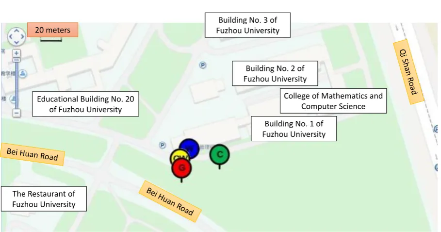
Abstract: This study proposes a mobile positioning method which adopts recurrent neural network algorithms to analyze the received signal strength indications from heterogeneous networks (e.g., cellular networks and Wi-Fi networks) for estimating the locations of mobile stations. The recurrent neural networks with multiple consecutive timestamps can be applied to extract the features of time series data for the improvement of location estimation. In practical experimental environments, there are 4,525 records, 59 different base stations, and 582 different Wi-Fi access points detected in Fuzhou University in China. The lower location errors can be obtained by the recurrent neural networks with multiple consecutive timestamps (e.g., 2 timestamps and 3 timestamps); the experimental results can be observed that the average error of location estimation was 9.19 meters by the proposed mobile positioning method with 2 timestamps.
Keywords: deep learning; recurrent neural networks; mobile positioning method; fingerprinting positioning method; received signal strength
1. Introduction
With the development of wireless networks and mobile networks, the techniques of
location-based services (LBS) can provide the corresponding services to the users according to users’ current
locations. LBS which have played an important role in many fields require the high accuracy of positioning technology [1-23].
For the LBS in outdoor environments, global positioning system (GPS) and assisted GPS (A-GPS) are popular techniques and meet most of the positioning requirements. However, these techniques may be no longer applicable if the problems of multi-path propagation of wireless signals exist [20]. Furthermore, higher power consumptions are required by these techniques [1]. Therefore, some studies proposed cellular-based positioning methods to analyze the signals of cellular networks for location estimation [1, 6, 8, 11, 13, 14]. Although cellular-based positioning methods can estimate the locations of mobile stations without GPS modules, big errors of estimated locations may be obtained.
For the LBS in indoor environments, Wi-Fi-based positioning methods are popular techniques to detect and analyze the received signal strength indications (RSSIs) from Wi-Fi access points (APs) [7, 12, 14, 18-22]. The fingerprinting positioning methods based on machine learning algorithms were proposed to learning the relationships among locations and RSSIs for the estimation of locations. Although these methods can estimate the locations of mobile stations without GPS modules, big errors of estimated locations may be obtained. Although higher precise estimated locations can be obtained by Wi-Fi-based positioning methods, these methods may be invalid in outdoor environments if the transmission coverage of Wi-Fi APs is not enough.
Some deep learning methods (e.g., neural networks, convolutional neural networks, recurrent neural networks, etc.) have been applied to improve the accuracies of estimation locations [12, 18, 19, 20, 22]. For instance, a modified probability neural network was used for indoor positioning, and the
accuracies of estimated locations by the method were higher than triangulation technique [18]. An improved neural network was trained with the correlation of the initial parameters to achieve the highest possible accuracy of the Wi-Fi-based positioning method in indoor environments [12].
Although cellular-based positioning methods can obtain estimated locations in outdoor environments, the errors of estimated locations may be larger. Furthermore, Wi-Fi-based positioning methods can obtain higher precise locations, but these methods may be not applicable in outdoor environments. Therefore, this study proposed a mobile positioning method to analyze the network signals from heterogeneous networks (e.g., cellular networks and Wi-Fi networks) for the LBS in outdoor environments. Furthermore, the recurrent neural networks [24] are applied into the proposed mobile positioning method for the analyses of consecutive locations and network signals (i.e., time series data).
The remainder of the paper is organized as follows. Section 2 provides the overview of mobile positioning methods and fingerprinting positioning methods. Section 3 presents the proposed mobile positioning system and method based on recurrent neural networks. The practical experimental results and discussions are illustrated in Section 4. Finally, conclusions and future work are given in Section 5.
2. Related Work
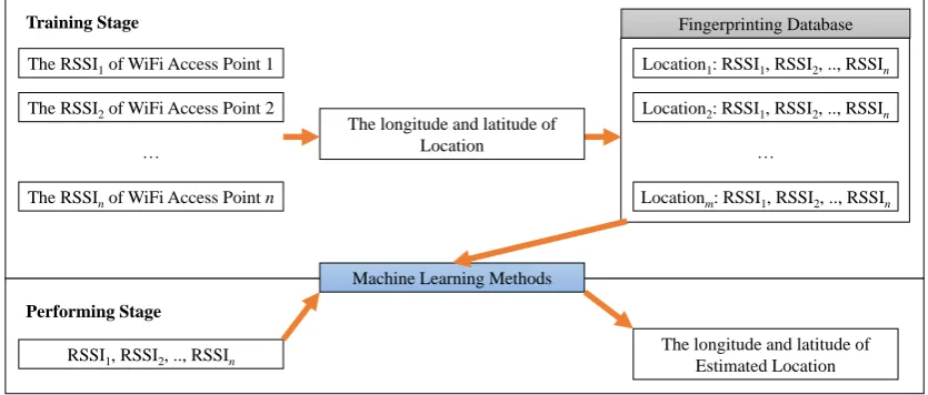
Mobile positioning methods and fingerprinting positioning methods includes two stages: training stage and performing stage (shown in Figure 1). In training stage, the RSSIs and locations measured by the mobile stations are matched and stored into a fingerprinting database for training. Machine learning methods can be performed to learn the relationships among RSSIs and locations for the establishments of mobile positioning models. In performing stage, mobile stations can detect the RSSIs of neighbor base stations and Wi-Fi APs which can be adopted into the trained models to estimate the locations of these mobile stations.
Figure 1. Fingerprinting positioning method
For training the mobile positioning models, some studies used k–nearest neighbors, Bayesian
theory, support vector machine, neural networks, convolutional neural networks, or recurrent neural networks to estimate locations in accordance with RSSIs. For instance, a probabilistic positioning algorithm was proposed to store the probability distribution of RSSIs during a certain time in the fingerprinting database, and the probable locations of mobile stations were calculated by a Bayesian theory system [14]. However, the relationships among inputs were assumed as independent parameters, so big errors of estimated locations may be obtained if the inputs were not independent
parameters. Some mobile positioning methods based on k–nearest neighbor algorithms can obtain
higher accuracies of estimated locations, but these methods required more computation time in performing stage. Some neural networks have been proposed to analyze the interrelated influences of inputs for the improvement of location estimation [12, 18-20], and convolutional neural networks
The RSSI1of WiFi Access Point 1 The RSSI2of WiFi Access Point 2
…
The RSSInof WiFi Access Point n
The longitude and latitude of Location
Location2: RSSI1, RSSI2, .., RSSIn Location1: RSSI1, RSSI2, .., RSSIn
…
Locationm: RSSI1, RSSI2, .., RSSIn Fingerprinting Database
RSSI1, RSSI2, .., RSSIn
Machine Learning Methods
The longitude and latitude of Estimated Location
Training Stage
were applied to extract the features of spatio metrics [21]. Although the spatio metrics may be analyzed by neural networks and convolutional neural networks, these methods cannot provide the solutions of temporal data analyses. Therefore, this study applies recurrent neural networks to analyze the temporal data for improving the accuracies of estimation locations.
3. Mobile Positioning System and Method
The architecture of the proposed mobile positioning system is presented in Subsection 3.1, and the concepts of the proposed mobile positioning method are illustrated in Subsection 3.2.
3.1. Mobile Positioning System
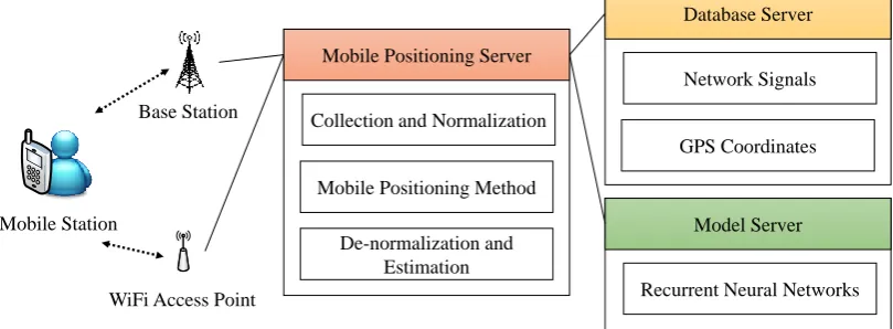
The proposed mobile positioning system includes (1) mobile stations, (2) a mobile positioning server, (3) a database server, and (4) a model server (shown in Figure 2). Each component in the proposed system is presented in the following subsections.
Figure 2. The proposed mobile positioning system 3.1.1. Mobile Stations
In training stage, mobile stations can detect and receive the RSSIs of neighbor base stations and Wi-Fi APs from heterogeneous networks. GPS modules can be equipped into the mobile stations and estimate the locations of mobile stations (i.e., coordinates). Then the mobile stations can send the vectors of GPS coordinates (i.e., longitudes and latitudes) and RSSIs to the mobile positioning server for the collection of network signals. In performing stage, mobile stations can send the detected RSSIs of neighbor base stations and Wi-Fi APs to the mobile positioning server for location estimation.
3.1.2. Mobile Positioning Server
In training stage, the mobile positioning server can receive GPS coordinates and network signals (i.e., the RSSIs of base stations and Wi-Fi APs) from mobile stations. These GPS coordinates and network signals can be sent to the database server for storing. The mobile positioning server can execute the proposed mobile positioning method to train RNN models. The network signals can be used as the input layer of the RNN models, and the GPS coordinates can be used as the output layer of the RNN models. Once the RNN models have been trained, these models can be sent to the model server for saving. In performing stage, the mobile positioning server can load the trained RNN models from the model server. When the mobile positioning server receives network signals from mobile stations, these network signals can be adopted into the trained RNN models for estimating the locations of mobile stations.
3.1.3. Database Server
Mobile Station
Base Station
WiFi Access Point
Mobile Positioning Server
Collection and Normalization
Mobile Positioning Method De-normalization and
Estimation
Database Server
Network Signals
GPS Coordinates
Model Server
The database server can store the vectors of coordinates (i.e., longitudes and latitudes) and RSSIs from mobile stations via the mobile positioning server. These vectors can be queried and used to train RNN models.
3.1.4. Model Server
The model server can save the trained RNN models from the mobile positioning server in training stage, and the saved RNN models can be loaded for location estimation by the mobile positioning server.
3.2. Mobile Positioning Method
The proposed mobile positioning method includes (1) collection and normalization, (2) the execution of mobile positioning method based on recurrent neural networks, (3) de-normalization and estimation. Each step in the proposed method is presented in the following subsections.
3.2.1. Collection and Normalization
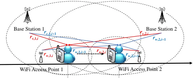
For the collection of network signals and GPS coordinates, the RSSIs of base stations from cellular networks (i.e.,
R
c i, in Equation (1)), the RSSIs of Wi-Fi APs from Wi-Fi networks (i.e.,R
w i,in Equation (2)), and the GPS coordinates (i.e.,
l
i in Equation (3)) can be detected and collected bythe mobile station at time
t
i (shown in Figure 3). The RSSI of the j-th base station from a cellularnetwork at time
t
i is defined asr
c j i, , , and the RSSI of the k-th Wi-Fi AP from a Wi-Fi network attime
t
i is defined asr
w k i, , . The RSSI dataset of heterogeneous networks (i.e., cellular networks andWi-Fi networks) at time
t
i is defined asR
i (shown in Equation (4)). Furthermore, the locationl
i(i.e., a GPS coordinate) includes a longitude
l
x i, and a latitudel
y i, . There are m locations, n1different base stations, and n2 different Wi-Fi APs detected in the experiments. If the RSSIs of base
stations or Wi-Fi APs cannot be detected, the values of these RSSIs can be encoded as null. For
instance, the mobile station cannot detect the RSSI of Wi-Fi AP2 at time
t
i in Figure 3, so the valueof
r
w,2,i is encoded as null.
1
, ,1,
,
,2,,...,
, ,c i c i c i c n i
R
=
r
r
r
(1)
2
, ,1,
,
,2,,...,
, ,w i w i w i w n i
R
=
r
r
r
(2)
,,
,
i x i y i
l
=
l
l
(3)
1 2
, ,
,1, ,2, , , ,1, ,2, , ,
,
,
,...,
,
,
,...,
i c i w i
c i c i c n i w i w i w n i
R
R
R
r
r
r
r
r
r
=
Figure 3. The scenario of network signal and GPS coordinate collection
For the normalization of network signals and GPS coordinates, the minimum values and maximum values of RSSIs and coordinates are considered and adopted into Equations (5), (6), (7), and (8). The normalized RSSI of the j-th base station from a cellular network at time
t
i is defined as,
j i
c
in accordance with the minimum value and maximum value of the RSSIs (i.e.,r
c( )−
and
r
c( )+
in Equation (5)) from cellular networks; the normalized RSSI of the k-th Wi-Fi APs from a cellular
network at time
t
i is defined asw
k i, in accordance with the minimum value and maximum valueof the RSSIs (i.e.,
r
w( )− andr
w( )+ in Equation (6)) from Wi-Fi networks. Furthermore, thenormalized longitude at time
t
i is defined asx
i in accordance with the minimum value andmaximum value of longitudes (i.e.,
l
x( )−
and
l
x( )+
in Equation (7)) from GPS coordinates, and the
normalized latitude at time
t
i is defined asy
i in accordance with the minimum value andmaximum value of latitudes (i.e.,
l
y( )−
and
l
y( )+
in Equation (8)) from GPS coordinates.
( )
( ) ( ) ( ) ( )
1 1
, ,
, ,
, , , , ,
1 ,1 1 ,1
,if
, where
max
,
min
0,otherwise
c j i c
c j i
j i c c c c p q c c p q
p n q m
p n q m
r
r
r
null
c
r
r
r
r
r
r
−
+ −
+ −
−
=
−
=
=
(5)
( )
( ) ( ) ( ) ( )
2 2
, ,
, ,
, , , , ,
1 ,1 1 ,1
,if
, where
max
,
min
0,otherwise
w k i w
w k i
k i w w w w p q w w p q
p n q m
p n q m
r
r
r
null
w
r
r
r
r
r
r
−
+ −
+ −
−
=
−
=
=
(6)
( )
( ), ( ) , ( ) ( )
, ,
1 1
,if
, where
max
,
min
0,otherwise
x i x
x i
i x x x x q x x q
q m q m
l
l
l
null
x
l
l
l
l
l
l
−
+ −
+ −
−
=
−
=
=
(7)
( )
( ), ( ) , ( ) ( )
, ,
1 1
,if
, where
max
,
min
0,otherwise
y i y
y i
i y y y q m y q y q m y q
l
l
l
null
y
l
l
l
l
l
l
−
+ −
+ −
−
=
−
=
=
(8)
Base Station 1 Base Station 2
WiFi Access Point 1 WiFi Access Point 2
Location liat time ti Location li+1at time ti+1
rc,1,i rc,1,i+1 r
w,2,i+1
rc,2,i
rw,1,i rw,2,i+1
3.2.2. Mobile Positioning Method Based on Recurrent Neural Network
The proposed mobile positioning method adopts recurrent neural network algorithms to estimate the locations of mobile stations. The recurrent neural networks can be applied to extract the features of time series data, so this study considers and analyzes the normalized RSSIs with multiple consecutive timestamps. Subsection 3.2.2.1 presents recurrent neural networks with one timestamp, and Subsection 3.2.2.2 describes recurrent neural networks with multiple consecutive timestamps.
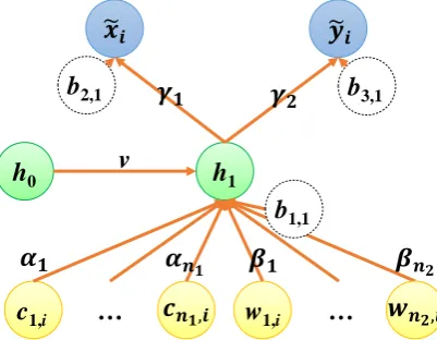
3.2.2.1. Recurrent Neural Networks with One Timestamp
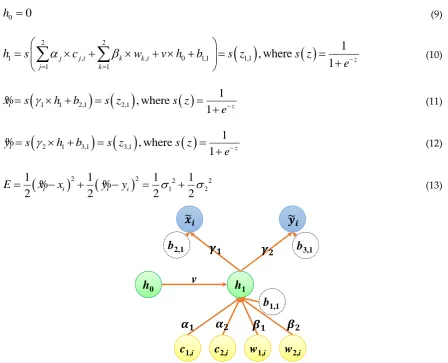
This subsection shows the designs and optimization of recurrent neural networks with one timestamp. A simple case study of a recurrent neural network with one timestamp is illustrated in Figure 4. The recurrent neural network is constructed with an input layer, a recurrent hidden layer, and an output layer. The input layer includes the normalized RSSIs of two base stations and two Wi-Fi APs (i.e., c1,i, c2,i, w1,i, and w2,i), and the output layer includes the estimated normalized longitude
and latitude (i.e.,
x
%
i andy
%
i). The recurrent hidden layer includes a neuron, and the initial value ofthe neuron in the recurrent hidden layer is defined as h0. The value of the neuron in the recurrent
hidden layer can be updated as h1 after calculating the RSSIs in the first timestamp. The weights of
c1,i, c2,i, w1,i, w2,i , and h0 are
1,2
,
1,
2, and v; the weights of h1 for the outputsx
%
i andy
%
i are1
and
2, respectively. The biases of neurons in the hidden layer and the output layer are definedas b1,1, b2,1, and b3,1. The sigmoid function is elected as the activation function of each neuron, so the
values of h0, h1,
x
%
i, andy
%
i can be calculated by Equations (9), (10), (11), and (12). Furthermore, theloss function is defined as Equation (13) in accordance with squared errors.
0
0
h
=
(9)( )
( )
2 2
1 , , 0 1,1 1,1
1 1
1
, where
1
j j i k k i z
j k
h
s
c
w
v h
b
s z
s z
e
−= =
=
+
+ +
=
=
+
(10)(
1 1 2,1) ( )
2,1( )
1
, where
1
i z
x
s
h
b
s z
s z
e
−=
+
=
=
+
%
(11)(
2 1 3,1) ( )
3,1( )
1
, where
1
i z
y
s
h
b
s z
s z
e
−=
+
=
=
+
%
(12)(
)
2(
)
2 2 21 2
1
1
1
1
2
i i2
i i2
2
E
=
x
%
−
x
+
y
%
−
y
=
+
(13)Figure 4. A recurrent neural network with one timestamp
h
1c
1,ic
2,iw
1,iw
2,ih
0v
For the optimization of recurrent neural network, the learning rate
and a gradient descentmethod is applied to update each weight and bias. The updates of
1,
2,b
2,1,b
3,1,
1,
2,
1,2
,v
, andb
1,1 are proved and calculated by Equations (14), (15), (16), (17), (18), (19), (20), (21), (22), and (23), respectively.
1 1
1
2,1 3,1
1 2
1 1 2,1 1 2 3,1 1
1 1
, where
1
i i i i i iE
z
z
x
y
E
E
E
x
z
y
z
x
x
h
= −
=
+
=
−
%
%
%
%
%
%
(14)
2 2 21, 2,1 2 3,1
2 1 2,1 2 2 3,1 2
2 1
, where
1
i i i i i iE
z
z
x
y
E
E
E
x
z
y
z
y
y
h
=
−
=
+
=
−
%
%
%
%
%
%
(15)
2,1 2,1 2,1 2,1 3,1 1 22,1 1 2,1 2,1 2 3,1 2,1
1
, where
1
i i i i i iE
b
b
b
z
z
x
y
E
E
E
b
x
z
b
y
z
b
x
x
=
−
=
+
=
−
%
%
%
%
%
%
(16)
3,1 3,1 3,1 2,1 3,1 1 23,1 1 2,1 3,1 2 3,1 3,1
2
, where
1
i i i i i iE
b
b
b
z
z
x
y
E
E
E
b
x
z
b
y
z
b
y
y
=
−
=
+
=
−
%
%
%
%
%
%
(17) 1 1 12,1 1,1 3,1 1,1
1 1 2 1
1 1 2,1 1 1,1 1 2 3,1 1 1,1 1
2,1 3,1
1 2 1
1 2,1 1 2 3,1 1 1,1
, where
i i i i i i i i
E
z
z
z
z
x
h
y
h
E
E
E
x
z
h
z
y
z
h
z
z
z
x
y
h
E
E
x
z
h
y
z
h
z
=
−
=
+
=
+
%
%
%
%
%
%
%
%
1,1 11 1 2 2 1 1 1,
i
1
i i1
i1
iz
x
x
y
y
h
h
c
=
−
%
%
+
−
%
%
−
2 2
2
2,1 1,1 3,1 1,1
1 1 2 1
2 1 2,1 1 1,1 2 2 3,1 1 1,1 2
2,1 3,1
1 2 1
1 2,1 1 2 3,1 1 1,1
, where
i i i i i i i i
E
z
z
z
z
x
h
y
h
E
E
E
x
z
h
z
y
z
h
z
z
z
x
y
h
E
E
x
z
h
y
z
h
z
=
−
=
+
=
+
%
%
%
%
%
%
%
%
1,1 21 1 2 2 1 1 2,
i
1
i i1
i1
iz
x
x
y
y
h
h
c
=
−
%
%
+
−
%
%
−
(19) 1 1 12,1 1,1 3,1 1,1
1 1 2 1
1 1 2,1 1 1,1 1 2 3,1 1 1,1 1
2,1 3,1
1 2 1
1 2,1 1 2 3,1 1 1,1
, where
i i i i i i i i
E
z
z
z
z
x
h
y
h
E
E
E
x
z
h
z
y
z
h
z
z
z
x
y
h
E
E
x
z
h
y
z
h
z
=
−
=
+
=
+
%
%
%
%
%
%
%
%
1,1 11 1 2 2 1 1 1,
i
1
i i1
i1
iz
x
x
y
y
h
h
w
=
−
%
%
+
−
%
%
−
(20) 2 2 22,1 1,1 3,1 1,1
1 1 2 1
2 1 2,1 1 1,1 2 2 3,1 1 1,1 2
2,1 3,1
1 2 1
1 2,1 1 2 3,1 1 1,1
, where
i i i i i i i i
E
z
z
z
z
x
h
y
h
E
E
E
x
z
h
z
y
z
h
z
z
z
x
y
h
E
E
x
z
h
y
z
h
z
=
−
=
+
=
+
%
%
%
%
%
%
%
%
1,1 21 1 2 2 1 1 2,
i
1
i i1
i1
iz
x
x
y
y
h
h
w
=
−
%
%
+
−
%
%
−
(21)
2,1 1,1 3,1 1,1
1 1 2 1
1 2,1 1 1,1 2 3,1 1 1,1
2,1 3,1 1,1
1 2 1
1 2,1 1 2 3,1 1 1,1
, where
i i i i i i i i
E
v
v
v
z
z
z
z
x
h
y
h
E
E
E
v
x
z
h
z
v
y
z
h
z
v
z
z
z
x
y
h
E
E
x
z
h
y
z
h
z
v
= −
=
+
=
+
%
%
%
%
%
%
%
%
1 1 2 2
1
1
0=
−
x
%
i1
x
%
i +
−
y
%
i1
y
%
i
−
h
1
h
h
1,1 1,1
1,1
2,1 1,1 3,1 1,1
1 1 2 1
1,1 1 2,1 1 1,1 1,1 2 3,1 1 1,1 1,1
2,1 3,1
1 2
1 2,1 1 2 3,1 1
, where
i i i i i i i i
E
b
b
b
z
z
z
z
x
h
y
h
E
E
E
b
x
z
h
z
b
y
z
h
z
b
z
z
x
y
E
E
x
z
h
y
z
h
=
−
=
+
=
+
%
%
%
%
%
%
%
%
1,1 1 1,1 1,11 1 2 2 1 1
i
1
i i1
i1
z
h
z
b
x
x
y
y
h
h
=
−
%
%
+
−
%
%
−
(23)For the generalization of recurrent neural network, the number of base stations and the number of Wi-Fi APs can be extended as n1 and n2 in the input layer (shown in Figure 5). The value of h1 can
be revised and calculated by Equation (24); the updates of
j and
k are proved and calculatedby Equations (25) and (26), respectively.
( )
( )
1 2
1 , , 0 1,1 1,1
1 1
1
, where
1
n n
j j i k k i z
j k
h
s
c
w
v h
b
s z
s z
e
− = =
=
+
+ +
=
=
+
(24)2,1 1,1 3,1 1,1
1 1 2 1
1 2,1 1 1,1 1 2 3,1 1 1,1
2,1 3,1
1 2 1
1 2,1 1 2 3,1 1 1,1
, where
j j
j
i i
j i i j
i i
i i
E
z
z
z
z
x
h
y
h
E
E
E
x
z
h
z
y
z
h
z
z
z
x
y
h
E
E
x
z
h
y
z
h
z
=
−
=
+
=
+
%
%
%
%
%
%
%
%
1,11 1 2 2 1 1 ,
1
1
1
j
i i i i j i
z
x
x
y
y
h
h
c
=
−
%
%
+
−
%
%
−
(25)
2,1 1,1 3,1 1,1
1 1 2 1
1 2,1 1 1,1 2 2 3,1 1 1,1
2,1 3,1
1 2 1
1 2,1 1 2 3,1 1 1,1
, where
k k
k
i i
k i i k
i i
i i
E
z
z
z
z
x
h
y
h
E
E
E
x
z
h
z
y
z
h
z
z
z
x
y
h
E
E
x
z
h
y
z
h
z
=
−
=
+
=
+
%
%
%
%
%
%
%
%
1,11 1 2 2 1 1 ,
1
1
1
k
i i i i k i
z
x
x
y
y
h
h
w
=
−
%
%
+
−
%
%
−
Figure 5. A generalized recurrent neural network with one timestamp
Furthermore, the number of neurons in the recurrent hidden layer can be extended for the extraction of time series data. The weight between each two neurons can be updated by the gradient descent method.
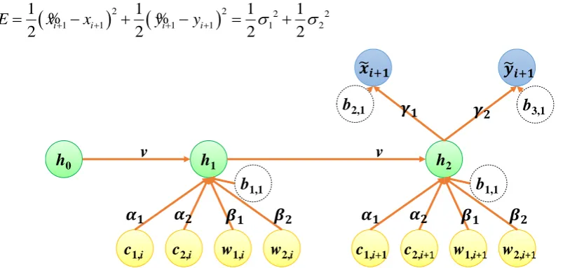
3.2.2.2. Two Timestamps for Recurrent Neural Network
This subsection illustrates the designs and optimization of recurrent neural networks with two consecutive timestamps. A simple case study of a recurrent neural network with two consecutive timestamps is showed in Figure 6. In the case, the recurrent neural network is constructed with an input layer, a recurrent hidden layer, and an output layer. The input layer includes four normalized RSSIs (i.e., c1,i, c2,i, w1,i, and w2,i) in the first timestamp and four normalized RSSIs (i.e., c1,i+1, c2,i+1, w1,i+1,
and w2,i+1) in the second timestamp; the output layer includes the estimated normalized longitude and
latitude (i.e.,
x
%
i+1 andy
%
i+1) in the second timestamp. The recurrent hidden layer includes a neuron,and the initial value of the neuron in the recurrent hidden layer is defined as h0 (shown in Equations
(9)). The value of the neuron in the recurrent hidden layer can be updated as h1 in the first timestamp
and be updated as h2 in the second timestamp. The weights of Base Station 1, Base Station 2, Wi-Fi
AP 1, and Wi-Fi AP in each timestamp are
1,
2,
1, and
2; the weights of h2 for the outputs1
i
x
%
+ andy
%
i+1 are
1 and
2, respectively. Furthermore, the weight of the neurons in the recurrenthidden layer in least timestamp is defined as v. In the case, the biases of neurons in the hidden layer
and the output layer are defined as b1,1, b2,1, and b3,1. The sigmoid function is elected as the activation
function of each neuron, so the values of h1, h2,
x
%
i, andy
%
i can be calculated by Equations (27), (28),(29), and (30). Furthermore, the loss function is defined as Equation (31) in accordance with squared errors.
( )
( )
2 2
1 , , 0 1,1 1,1
1 1
1
, where
1
j j i k k i z
j k
h
s
c
w
v h
b
s z
s z
e
−= =
=
+
+ +
=
=
+
(27)( )
( )
2 2
2 , 1 , 1 1 1,1 1,2
1 1
1
, where
1
j j i k k i z
j k
h
s
c
w
v h
b
s z
s z
e
+
+ −= =
=
+
+ +
=
=
+
(28)(
) ( )
( )
1 1 2 2,1 2,1
1
, where
1
i z
x
s
h
b
s z
s z
e
+
=
+
=
=
+
−%
(29)(
) ( )
( )
1 2 2 3,1 3,1
1
, where
1
i z
y
s
h
b
s z
s z
e
+
=
+
=
=
+
−%
(30)h
1…
w
1,i…
h
0v
b
3,1b
2,1c
1,i(
)
2(
)
2 2 21 1 1 1 1 2
1
1
1
1
2
i i2
i i2
2
E
=
x
%
+−
x
++
y
%
+−
y
+=
+
(31)Figure 6. A recurrent neural network with two consecutive timestamps
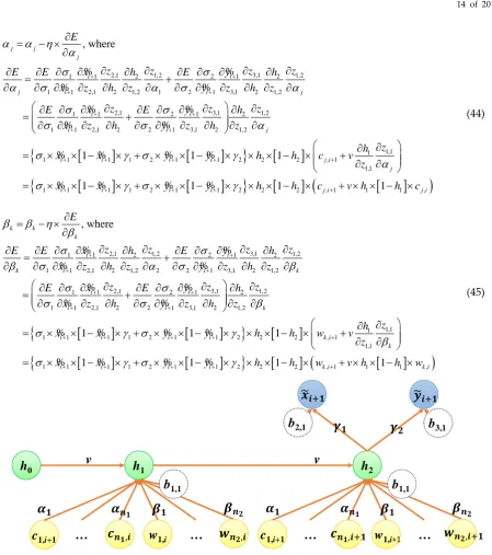
For the optimization of recurrent neural network with two consecutive timestamps, the learning
rate
and a gradient descent method is applied to update each weight and bias. The updates of
1,
2,b
2,1,b
3,1,
1,
2,
1,
2,v
, andb
1,1 are proved and calculated by Equations (32), (33),(34), (35), (36), (37), (38), (39), (40), and (41), respectively.
1 1
1
2,1 3,1
+1 +1
1 2
1 1 +1 2,1 1 2 +1 3,1 1
1 +1 +1 2
, where
1
i i
i i
i i
E
z
z
x
y
E
E
E
x
z
y
z
x
x
h
= −
=
+
=
−
%
%
%
%
%
%
(32)
2 2
2
1, +1 2,1 2 +1 3,1
2 1 +1 2,1 2 2 +1 3,1 2
2 +1 +1 2
, where
1
i i
i i
i i
E
z
z
x
y
E
E
E
x
z
y
z
y
y
h
=
−
=
+
=
−
%
%
%
%
%
%
(33)
2,1 2,1
2,1
2,1 3,1
+1 +1
1 2
2,1 1 +1 2,1 2,1 2 +1 3,1 2,1
1 +1 +1
, where
1
i i
i i
i i
E
b
b
b
z
z
x
y
E
E
E
b
x
z
b
y
z
b
x
x
=
−
=
+
=
−
%
%
%
%
%
%
(34)
h
0h
1c
1,ic
2,iw
1,iw
2,iv
b
1,1h
2c
1,i+1c
2,i+1w
1,i+1w
2,i+1v
3,1 3,1 3,1 2,1 3,1 +1 +1 1 23,1 1 +1 2,1 3,1 2 +1 3,1 3,1
2 +1 +1
, where
1
i i i i i iE
b
b
b
z
z
x
y
E
E
E
b
x
z
b
y
z
b
y
y
=
−
=
+
=
−
%
%
%
%
%
%
(35) 1 1 12,1 1,2 3,1 1,2
+1 +1
1 2 2 2
1 1 +1 2,1 2 1,2 1 2 +1 3,1 2 1,2 1
2,1 3,1
+1 +1
1 2
1 +1 2,1 2 2 +1 3,1 2
, where i i i i i i i i E
z z z z
x h y h
E E E
x z h z y z h z
z z
x y
E E
x z h y z h
= − = + = + % % % % % % % %
(
)
1,2 2 1,2 1 1,1 11 +1 +1 1 2 +1 +1 2 2 2 1, 1
1,1 1
1 +1 +1 1 2 +1 +1 2 2 2 1, 1 1 1 1,
1 1 1
1 1 1 1
i i i i i
i i i i i i
z h z
z h
x x y y h h c v
z
x x y y h h c v h h c
+ + = − + − − + = − + − − + − % % % % % % % % (36) 2 2 2
2,1 1,2 3,1 1,2
+1 +1
1 2 2 2
2 1 +1 2,1 2 1,2 2 2 +1 3,1 2 1,2 2
2,1 3,1
+1 +1
1 2
1 +1 2,1 2 2 +1 3,1 2
, where i i i i i i i i E
z z z z
x h y h
E E E
x z h z y z h z
z z
x y
E E
x z h y z h
= − = + = + % % % % % % % %
(
)
1,2 2 1,2 2 1,1 11 +1 +1 1 2 +1 +1 2 2 2 2, 1
1,1 2
1 +1 +1 1 2 +1 +1 2 2 2 2, 1 1 1 2,
1 1 1
1 1 1 1
i i i i i
i i i i i i
z h z
z h
x x y y h h c v
z
x x y y h h c v h h c
+ + = − + − − + = − + − − + − % % % % % % % % (37) 1 1 1
2,1 1,2 3,1 1,2
+1 +1
1 2 2 2
1 1 +1 2,1 2 1,2 1 2 +1 3,1 2 1,2 1
2,1 3,1
+1 +1
1 2
1 +1 2,1 2 2 +1 3,1 2
, where i i i i i i i i E
z z z z
x h y h
E E E
x z h z y z h z
z z
x y
E E
x z h y z h
= − = + = + % % % % % % % %
(
)
1,2 2 1,2 1 1,1 11 +1 +1 1 2 +1 +1 2 2 2 1, 1
1,1 1
1 +1 +1 1 2 +1 +1 2 2 2 1, 1 1 1 1,
1 1 1
1 1 1 1
i i i i i
i i i i i i
z h z
z h
x x y y h h w v
z
x x y y h h w v h h w