Article
1
Time Series Forecasting using a Two-level
Multi-2
objective Genetic Algorithm: A case study of
3
maintenance cost data for tunnel fans
4
Yamur K. Al-Douri 1,*, Hussan Hamodi 2 and Jan Lundberg 3
5
1 Ph.D. candidate, Division of Operation and Maintenance Engineering, Luleå University of Technology,
SE-6
97187 Luleå, Sweden; yamur.aldouri@ltu.se
7
2 Ph.D., Division of Operation and Maintenance Engineering, Luleå University of Technology, SE-97187
8
Luleå, Sweden. Mechanical Engineering Department, College of Engineering, University of Mosul, Mosul,
9
Iraq; hussan.hamodi@ltu.se
10
3 Division of Operation and Maintenance Engineering, Luleå University of Technology, SE-97187 Luleå,
11
Sweden, jan.lundberg@ltu.se
12
* Correspondence: yamur.aldouri@ltu.se; Tel.: +46-7-2247-4992
13
14
Abstract: The aim of this study has been to develop a novel two-level multi-objective genetic
15
algorithm (GA) to optimize time series forecasting data for fans used in road tunnels by the Swedish
16
Transport Administration (Trafikverket). Level 1 is for the process of forecasting time series cost
17
data, while level 2 evaluates the forecasting. Level 1 implements either a multi-objective GA based
18
on the ARIMA model or a multi-objective GA based on the dynamic regression model. Level 2
19
utilises a multi-objective GA based on different forecasting error rates to identify a proper
20
forecasting. Our method is compared with using the ARIMA model only. The results show the
21
drawbacks of time series forecasting using only the ARIMA model. In addition, the results of the
22
two-level model show the drawbacks of forecasting using a multi-objective GA based on the
23
dynamic regression model. A multi-objective GA based on the ARIMA model produces better
24
forecasting results. In level 2, five forecasting accuracy functions help in selecting the best
25
forecasting. Selecting a proper methodology for forecasting is based on the averages of the
26
forecasted data, the historical data, the actual data and the polynomial trends. The forecasted data
27
can be used for life cycle cost (LCC) analysis.
28
Keywords: ARIMA model, Data forecasting, Multi-objective genetic algorithm, Regression model
29
30
1. Introduction
31
Time series forecasting predicts future data points based on observed data over a period known
32
as the lead-time. The purpose of forecasting data points is to provide a basis for economic planning,
33
production planning, production control and optimizing industrial processes. The major objective is
34
to obtain the best forecast function, i.e. to ensure that the mean square of the deviation between the
35
actual and the forecasted values is as small as possible for each lead-time [1]. Much effort has been
36
devoted over the past few decades to the development and improvement of time series forecasting
37
models [2].
38
Traditional models for time series forecasting, such as the Box–Jenkins or autoregressive
39
integrated moving average (ARIMA) model, assume that the studied time series are generated from
40
linear processes. However, these models may be inappropriate if the underlying mechanism is
41
nonlinear. In fact, real-world systems are often nonlinear [3]. The multi-objective genetic algorithm
42
(GA) is often compatible with nonlinear systems and uses a particular optimization from the principle
43
of natural selection of the optimal solution on a wide range of forecasting populations [4].
44
The proposed multi-objective GA optimizes a particular function based on the ARIMA model.
45
The ARIMA model is a stochastic process modelling framework [1] that is defined by three
46
parameters ( , , ). The parameter stands for the order of the autoregressive ( ) process,
47
for the order of integration (needed for the transformation into a stationary stochastic process), and
48
for the order of the moving average ( ) process [5]. A stationary stochastic process means a
49
process where the data properties have the same variance and autocorrelation [6]. The weakness of
50
the ARIMA model is the difficulty of estimating the parameters. To address this problem, a process
51
for automated model selection needs to be implemented in the automated optimization to achieve an
52
accurate forecasting [7].
53
The GA is a well-established method which helps in solving complex and nonlinear problems
54
that often lead to cases where the search space shows a curvy landscape with numerous local minima.
55
The multi-objective GA is designed to find the best forecasting solution through automated
56
optimization of the ARIMA model and to select the best parameters ( , , ) to compute point
57
forecasts based on time series data. The parameters of the ARIMA model are influenced by the
58
selecting process of the GA. In addition, the multi-objective GA can evaluate the forecasting accuracy
59
using multiple fitness functions based on statistics models.
60
Vantuch & Zelinka [8] modified the ARIMA model based on the genetic algorithm and particle
61
swarm optimization (PSO) to estimate and predict data of time. They found that the genetic algorithm
62
could find a suitable ARIMA model and pointed to improvements through individual binary
63
randomization for every parameter input of the ARIMA model. Their model shows the best set of
64
coefficients obtained with PSO compared with the best set obtained with a classical ARIMA
65
prediction. However, these authors present the ARIMA parameters in a binary setting with limited
66
possibilities and they consider the forecasting based on an ARIMA evaluation only.
67
Wang & Hsu [9] proposed a combination of grey theory and the genetic algorithm to overcome
68
industrial development constraints and establish a high-precision forecasting model. They used a
69
genetic algorithm to optimize grey forecasting model parameters. They demonstrated a successful
70
application of their model which provided an accurate forecasting with a low forecasting error rate.
71
However, these authors proposed randomization in combination with grey theory without
72
integrating grey theory functionality within the GA. They used only one forecasting error rate to
73
judge the forecasting accuracy.
74
Ervural et al. [10] proposed a forecasting method based on an integrated genetic algorithm and
75
the ARMA model in order to gain the advantage of both of these tools in the forecasting of data. They
76
used a genetic algorithm to optimize ( ) and ( ) and find the best ARMA model for the
77
problem. They found that their model had an effective identification for estimating ARMA
78
autoregression and moving averages. However, these authors presented ARIMA parameters with
79
limited possibilities. In addition, they used only one forecasting error rate to judge the forecasting
80
accuracy.
81
Hatzakis & Wallace [4] proposed a method that combines the ARIMA forecasting technique and
82
a multi-objective GA based on the Pareto optimal to predict the next optimum. Their method is based
83
on historical optimums and is used to optimize ( ) and ( ) to find a non-dominated Pareto
84
front solution with an infinite number of points. They found that their method improved the
85
prediction accuracy. However, these authors assumed that the data were accurate and used the
86
Pareto front solution to select a proper forecasting. In addition, they did not use any forecasting error
87
rate to evaluate the forecasting results.
88
The aim of this study has been to develop a novel two-level multi-objective GA to optimize time
89
series forecasting in order to forecast cost data for fans used in road tunnels. The first level of the GA
90
is responsible for the process of forecasting time series cost data, while the second level evaluates the
91
forecasting. The first level implements either a multi-objective GA based on the ARIMA model or a
92
multi-objective GA based on the dynamic regression model. This level gives possibilities of finding
93
the optimal forecasting solution. The second level utilises a multi-objective GA based on different
94
forecasting error rates to identify a proper forecasting. Our method is compared with the approach
95
increases the flexibility, and is very effective when selecting an approximate solution interval for
97
forecasting.
98
2. Data collection
99
The cost data concern tunnel fans installed in Stockholm in Sweden. The data had been collected
100
over ten years from 2005 to 2015 by Trafikverket and were stored in the MAXIMO computerized
101
maintenance management system (CMMS). In this CMMS, the cost data are recorded based on the
102
work orders for the maintenance of the tunnel fans. Every work order contains corrective
103
maintenance data, a component description, the reporting date, a problem description, and a
104
description of the actions performed. Also included are the repair time used and the labour, material
105
and tool cost of each work order.
106
In this study, we consider the two cost objects of labour and materials based on the work order
107
input into the CMMS for the ten-year period mentioned above. The tool cost data were not selected
108
due to the huge number of missing data that could not be used for forecasting. The selected data were
109
clustered, filtered and imputed for the present study using a multi-objective GA based on a fuzzy
c-110
means algorithm. It is important to mention that all the cost data used in this study concern real costs
111
without any adjustment for inflation. Due to company regulations, all the cost data have been
112
encoded and are expressed as currency units (cu).
113
3. The ARIMA model
114
The main part of the ARIMA model concerns the combination of autoregression (AR) and
115
moving-average (MA) polynomials into a complex polynomial, as seen in the equation below [8]. The
116
ARIMA model is applied to all the data points for each cost data object (labour and material).
117
118
= + ∑ ( ) + ∑ ( ) + ,
119
120
where the notation is as follows:
121
: the mean value of the time series data;
122
: the number of autoregressive lags;
123
: the number of differences calculated with the equation ∆ = − ;
124
: the number of lags of the moving average process;
125
: autoregressive coefficients (AR);
126
: moving average coefficients (MA);
127
: the white noise of the time series data.
128
129
The value of the ARIMA parameters ( , , ) for AR and MA can be obtained from the
130
behaviour of the autocorrelation function (ACF) and the partial autocorrelation function (PACF) [1].
131
These functions help in estimating parameters that can be used to forecast data by using the ARIMA
132
model.
133
4. Two-level system of multi-objective genetic algorithms
134
In this study, a novel two-level multi-objective GA has been developed, as shown in Figure 1. The
135
levels of the GA are as follows: (1) a multi-objective GA based on the ARIMA model for forecasting
136
the cost data, and (2) a multi-objective GA based on multiple functions for measuring the forecasting
137
accuracy for validation of the forecasted data. Level 1 of the multi-objective GA is applied to the cost
138
data objects (labour and material) at four different times (four populations) to forecast data for the
139
next level and for each of 15 different generations. The second level validates the forecasted data for
140
the two cost objects. Using two levels allows us to reduce the computational cost [11], while reaching
141
143
Figure 1: Two-level system of multi-objective GAs.
144
4.1. Level 1: multi-objective GA based on the ARIMA model
145
The proposed multi-objective GA method uses a particular optimization based on the principle
146
of natural selection of the optimal solution and applies this optimization on a wide range of
147
forecasting populations. The multi-objective GA creates populations of chromosomes as possible
148
answers to estimate the optimum forecasting [4]. This algorithm is robust, generic and easily
149
adaptable because it can be broken down into the following steps: initialization, evaluation, selection,
150
Multi-objective GA based on the ARIMA model
80% training forecasting data
Data forecasted for each Population
Forecasting data for 15 different generations
L
ev
el
1
Multi-objective GA based on forecasting accuracy models
Validate
L
ev
el
2
Population (Pi)
Forecasting
Forecasting population
Optimal forecasting Encoding
Encoding
Time series data forecasting …
crossover, mutation, update and completion. The evaluation (fitness function) step creates the basis
151
for a new population of chromosomes. The new population is formed using specific genetic
152
operators, such as crossover and mutation [13, 14]. The fitness function is derived from the ARIMA
153
forecasting model. A GA with automated optimization avoids the weakness of the ARIMA model by
154
estimating the parameters for forecasting [7].
155
The multi-objective GA is a global optimization technique that can be used to achieve an accurate
156
forecasting based on the ARIMA model. The GA is known to help in solving complex nonlinear
157
problems that often lead to cases where the search space shows a curvy landscape with numerous
158
local minima. Moreover, the multi-objective GA is designed to find the optimal forecasting solution
159
through automated optimization of the ARIMA model. In addition, the multi-objective GA can
160
evaluate the forecasting accuracy using multiple fitness functions based on statistical models.
161
The first level utilises a multi-objective GA which is based on the ARIMA model and is
162
implemented four different times using a cross-validation randomization technique. The technique
163
aims to select the best time series data for forecasting. The process is the following: a random number
164
of cost data are selected based on encoding in each of the four implementations; the modified random
165
cost data are generated 15 times. The modifications are used to find the optimal cost data for
166
forecasting. The following steps are implemented when applying the multi-objective GA in level 1.
167
Step 1: Initial population
168
A longitudinal study of each cost object ( , ) is used to forecast data using the
169
multi-objective GA for the two objects in parallel.
170
Step 2: First GA generation and selection
171
The first generation is performed by selecting each cost object and checking whether the data
172
are stationary (i.e. trend-stationary) or non-stationary using a Dickey-Fuller test [15]. To apply the
173
ARIMA model, the data should be stationary, i.e. the null hypothesis of stationarity should not be
174
rejected. When applying the Dickey-Fuller test equation, the hypothesis p = 1 means that the data are
175
non-stationary and p < 1 that the data are stationary.[15].
176
The Dickey-Fuller test equation is as follows:
177
Dickey − Fuller test ( ) = + + ,
178
where the notation is as follows:
179
: constant estimated value of the time series data;
180
: the hypothesis is either = 1 or < 1;
181
: time {1, … , };
182
: the white noise of the time series data.
183
Step 3: Encoding
184
Random values, either ones or zeros, are generated for each cost data object. Encoding is the
185
process of transforming from the phenotype to the genotype space before proceeding with
multi-186
objective GA operators and finding the local optima.
187
The fitness function is based on the ARIMA model for the forecasting of time series cost data
189
objects individually, as seen in the equation below. The fitness function consists of an autoregression
190
(AR) part and a moving average (MA) part [1]. The ARIMA model uses AR and MA polynomials to
191
estimate ( ) and ( ) [8].
192
The fitness function is formulated as follows:
193
( , , ) = + ∑ ( ) + ∑ ( ) + ,
194
where the following notation is used:
195
: the mean value of the time series data;
196
: the number of autoregressive lags;
197
: the number of differences calculated with the equation ∆ = − ;
198
: the number of lags of the moving average process;
199
: autoregressive coefficients (AR);
200
: moving average coefficients (MA);
201
: the white noise of the time series data.
202
The parameters ( , ) are estimated using an autocorrelation function (ACF) and a partial
203
autocorrelation function (PACF) [1]. The estimated values produced by the previous equation will be
204
used to create a forecast for 20 months ( ) using the equation below [16]. These forecasted values
205
will be evaluated using the second level of multi-objective GA to find the optimal forecasting with
206
high accuracy.
207
( + ) = + ∑ ( ) + ∑ ( ) + ,
208
where ( + ) is the time series forecasting at time ( + ) and
209
: months {1, 2, 3,…, }.
210
Step 5: Crossover and mutation
211
In this study, a one-point crossover with a fixed crossover probability is used. This probability
212
decreases the bias of the results over different generations caused by the huge data values. For
213
chromosomes of length , a crossover point is generated in the range [1, 1/2 ] and [1/2 , ]. The
214
values of objects are connected and should be exchanged to produce two new offspring. We select
215
two points to create more value ranges and find the best fit.
216
Randomly, ten percent of the selected chromosomes undergo mutation with the arrival of new
217
chromosomes. For the cost object values, we swap two opposite data values. The purpose of this
218
small mutation percentage is to keep the forecasting changes steady over different generations.
219
Step 6: New generation
220
The new generation step repeats steps 3 to 5 continuously for 15 generations. Fifteen generations
221
are enough for these data because the curves of the fitness functions are repeated after fifteen
222
forecasting accuracy for each object and population. This step yields fully correlated data for the next
224
step.
225
4.2. Level 2: multi-objective GA for measuring the forecasting accuracy
226
In this level, the multi-objective GA is applied longitudinally to the data. The multi-objective GA
227
operates with a population of chromosomes that contains labour cost and material cost objects. The
228
GA operates on the selected population over different generations to find the appropriate forecasting
229
accuracy. During the GA generations, the chromosomes in the population are rated concerning their
230
adaptation, and their mechanism of selection for the new population is evaluated. Their adaptability
231
(fitness function) is the basis for a new population of chromosomes. The new population is formed
232
using specific genetic operators such as crossover and mutation. The multi-objective GA is used to
233
evaluate the forecasting accuracy for each generation of the first level.
234
Level 2 utilises a multi-objective GA which is based on different forecasting error rates and is
235
implemented for each generation from the first level and for four different populations using a
cross-236
validation randomization technique. This technique aims to select the best evaluation of the time
237
series data forecasting and the process is as follows. A random number of cost data are selected based
238
on the encoding in each generation of the four implementations, and the modified random cost data
239
are generated five times. The modifications are then used to find the optimal cost data forecasting. In
240
this study, due to the size of the training data, five generations are sufficient to obtain valid results.
241
The following steps are implemented when applying the multi-objective GA in level 2.
242
Step 1: Initial population
243
A longitudinal study is performed of each generation and each cost object ( , )
244
with its forecasted data using the multi-objective GA in parallel.
245
Step 2: First GA generation, encoding and selection
246
The first generation is performed by selecting each cost object and encoding through generating
247
random values, either ones or zeros, for each cost data object. The selection for each cost data object
248
is based on encodings with the value of 1. This selection is used to evaluate the forecasted data using
249
the multi-objective fitness function.
250
Step 3: Fitness function
251
The multi-objective fitness function is based on multiple functions for measuring the forecasting
252
accuracy. The mean absolute percentage error (MAPE), the median absolute percentage error
253
(MdAPE), the root mean square percentage error (RMSPE), the root median square percentage error
254
(RMdSPE), and the mean absolute scaled error (MASE) are different fitness functions used to evaluate
255
the selected forecasting data from the previous step [17]. The fitness functions are formulated as
256
follows:
257
(MAPE) = (| |) , where = = − ,
258
(MdAPE) = (| |) , where = = − ,
259
(RMSPE) = ( ) , where = = − ,
260
(RMdSPE) = ( ) , where = = − ,
(MASE) = (| |) , where =
∑ | |, where = − ;
262
in the above equations, the following notation is used:
263
: time {1, … , };
264
: the actual data over time;
265
: the forecasted data over time.
266
The MAPE is often substantially larger than the MdAPE when the data involve small counts. In
267
this study, it was impossible to use these measures since zero values of frequently occurred. The
268
RMSPE and RMdSPE are more sensitive to the data. These methods are examples of a random walk
269
and measure the accuracy based on the last adjusted observation of forecasted seasonality. The MASE
270
is a scaled measure based on relative errors. This module tries to remove the scale of the data by
271
comparing the forecasted data with data obtained from some benchmark forecast method [17].
272
Step 4: Crossover and mutation
273
In this study, we use a one-point crossover with a fixed crossover probability. This probability
274
decreases the bias of the results over different generations due to the huge data values. For
275
chromosomes of length , a crossover point is generated in the range [1, 1/2 ] and [1/2 , ]. The
276
values of objects are connected and should be exchanged to produce two new offspring. We select
277
two points to create more value ranges and find the best fit.
278
Randomly ten percent of the selected chromosomes undergo mutation with the arrival of new
279
chromosomes. For the cost object values, we swap two opposite data values. The purpose of this
280
small mutation percentage is to keep the forecasting changes steady over different generations.
281
Step 5: New generation
282
The new generation step repeats steps 2 to 4 continuously for five generations. Five generations
283
are enough for these data, because the fitness function is repeated after the fifth generation. The
284
selected generation is used for the second level to validate the forecasting accuracy for each object.
285
This step yields fully correlated data that can be used for forecasts covering several months.
286
5. Multi-objective genetic algorithms (GAs) based on the dynamic regression model
287
The study has developed a multi-objective GA based on the dynamic regression model. The
288
dynamic regression (DR) model differs from the ordinary regression model in that it can handle both
289
contemporaneous and time-lagged relationships [18]. The developed GA consists of the following
290
levels: (1) a objective GA based on the DR model and used to forecast cost data, and (2) a
multi-291
objective GA based on multiple functions for measuring the forecasting accuracy for the purpose of
292
validating the forecasted data. The multi-objective GA is applied to the cost data objects (labour and
293
material) for 15 different generations for four different populations to forecast data for the next level.
294
Then the forecasted data for the two cost objects are validated.
295
We use the same steps as those applied in the first level of the GA based on the ARIMA model,
296
applying them on the same data with the same method for every step. However, the fitness function
297
step is based on the regression model, as clarified below.
298
The multi-objective fitness function is based on the dynamic regression model function, as
300
expressed in the fitness equation below [18]. The fitness function is applied to a 20-month forecast.
301
The data have been normalized before calculating the fitness function. The purpose of the
302
normalization is to decrease the computation complexity, since the cost data values are huge. The
303
equation used for the normalization is as follows:
304
= ( − ) / ( − ).
305
The fitness equation is as follows:
306
fitness( ) = + + + ,
307
where the notation is as follows:
308
: constant value calculated with the normal equation, where = ;
309
: calculated with the normal equation, where = ;
310
: related to and ;
311
: white noise.
312
The results of the fitness function for the 20-month forecast are denormalized to the original data
313
using the equation below. The denormalization values are used to evaluate the forecasting accuracy
314
using the second level.
315
= ∗ − + .
316
The forecasting accuracy for every generation for every population is validated using the
multi-317
objective GA based on multiple functions for measuring the forecasting accuracy. The mean absolute
318
percentage error (MAPE), the median absolute percentage error (MdAPE), the root mean square
319
percentage error (RMSPE), the root median square percentage error (RMdSPE), and the mean
320
absolute scaled error (MASE) are different fitness functions used to evaluate the selected forecasting
321
data from the previous step [17]. The method used for validating the forecasting accuracy of the GA
322
based on the ARIMA model is used to validate the forecasting accuracy of the GA based on the
323
dynamic regression model.
324
6. Models evaluation method
325
A comparison of the three methods described above is performed based on the averages of the
326
historical data, the actual data and the polynomial trends. The polynomial trend is often used in many
327
applications and it was used in this study for the comparison of the models. The deviation average
328
of is calculated based on two different functions for every method. This provides a means of
329
comparing the different methods and finding a proper forecasting, i.e. a forecasting where the
330
deviation average is close to zero. This step confirms our judgement on the best forecasting method
331
for the data.
332
For each method and cost data object, the average is calculated for the historical data, , the
333
actual data, , the forecasted data, , and the polynomial data, . Figure 2 and 3 show the averages
334
calculated for the two cost objects of labour and materials. The average of the historical data (A) is
335
the average of the data before the vertical line. The average of the actual data (B) is the average of the
336
data after the vertical line. The average of the forecasted data (C) is the average of the forecasted data
337
after the vertical line. The average of the polynomial data (D) is the average of the polynomial data
338
deviation average DV1 ( ) = − ,
340
deviation average DV2 ( ) = ;
341
is the cost data object over time.
342
7. Results and discussion
343
7.1. Results of the ARIMA model
344
The ARIMA model was implemented stochastically based on the default values for the
345
parameters , and for the different scenarios and individually for each cost object ( ,
346
). The values assumed for each parameter in the scenarios were (1,1,1), (1,0,0), (1,0,1) and
347
(2,0,1). For every scenario, all the cost data points of each object were included, covering a period of
348
97 months. The scenarios do not show a reasonable forecasting for a period of 20 months for each
349
object. In this section, we present the cost object forecasting of the ARIMA model (1,1,1) as the default
350
input parameters.
351
Figure 2 shows the forecasting for the labour cost object with the polynomial trend to illustrate
352
the relationship between the values over a timeline with monthly intervals. Before the vertical line,
353
the historical labour cost data for 97 months are shown, and after the vertical line, the actual labour
354
cost data for 20 months are shown. The forecasted data for the 20-month period do not seem to be in
355
sync with the actual data and are lower than the trend of the data. The forecasting based on the
356
ARIMA model does not reflect the real data for the labour cost object.
357
358
Figure 2. Labour cost data forecasting based on the ARIMA model.
359
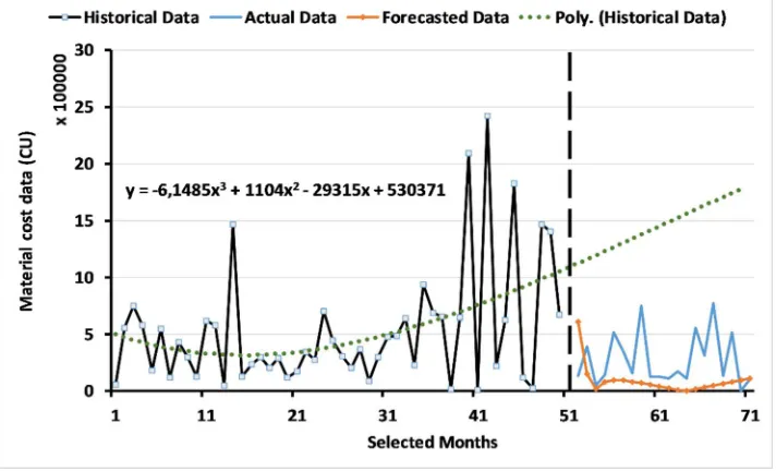
Figure 3 shows the forecasting for the material cost object with the polynomial trend to illustrate
360
the relationship between the values over a timeline with monthly intervals. Before the vertical line,
361
the historical material cost data for 97 months are presented, and after the vertical line, the actual
362
material cost data for 20 months are presented. The forecasted data for the 20-month period do not
363
seem to be in sync with the actual data and are lower than the trend of the data. The forecasting based
364
366
Figure 3. Material cost data forecasting based on the ARIMA model.
367
Overall, the forecasting based on the ARIMA model does not show sufficient accuracy over the
368
20-month period.
369
7.2. Results of the two-level system of multi-objective GAs
370
7.2.1 Results for level 1: multi-objective GA based on the ARIMA model
371
In this part of the study, we tested four populations individually using the multi-objective GA
372
based on the ARIMA model to generate forecasting data for the two different cost objects. The
373
forecasted data for each population obtained with 15 different generations were then evaluated using
374
the second level. The second level evaluation helped in deciding the best generation of the forecasted
375
data. In this section, we present only the best forecasted curves with the historical data because of the
376
huge number of possibilities considered in this study.
377
Figure 4 shows the forecasted labour data curve for 20 months from 2013 to 2015, for the second
378
population and, specifically, for generation 13. In addition, it shows the historical data with the
379
polynomial trend to illustrate the relationship between the independent variables over a timeline
380
with monthly intervals. The selected labour data show a better forecasting than that obtained with
381
the ARIMA model in that the forecasted data are close to the actual data and the polynomial trend.
382
The ARIMA parameters for the selected labour cost data covering 47 months were = 0.22, = 1
383
385
Figure 4. Labour cost data forecasting using the multi-objective GA based on the ARIMA model.
386
Figure 5 shows the curve for the forecasted material data for 20 months from 2013 to 2015, for
387
the third population and, specifically, for generation 10. In addition, this figure shows the original
388
data with the polynomial trend to illustrate the relationship between the independent variables over
389
a timeline with monthly intervals. The selected material data show better forecasting than that
390
obtained with the ARIMA model in that the forecasted data are close to the actual data and the
391
polynomial trend. The ARIMA parameters for the selected material cost data covering 52 months
392
were = 0.39, = 1 and = 0.43.
393
394
Figure 5. Material cost data forecasting using the multi-objective GA based on the ARIMA model.
395
The forecasted data for the labour and material cost objects were evaluated using the second
396
level, applying a multi-objective GA based on the statistical forecasting error rate. The model for the
397
forecasting accuracy evaluated the forecasted data for 20 months from 2013 to 2015 based on the
398
actual values of this period. Implementing level 2, the accurate forecasted data were found, i.e. the
399
7.2.2 Results of level 2: multi-objective GA for measuring the forecasting accuracy
401
The outcome from the first level, specifically for each generation for each population, indicates
402
the forecasting accuracy for each cost object. For each generation, the multi-objective GA based on
403
multiple fitness functions was used to find the best fitness value through five different generations.
404
The fitness functions (forecasting error rate models) provide an accurate data forecasting through
405
comparing the behaviour of the different models and revealing which forecasting model is
406
appropriate.
407
Figures 6 and 7 show the forecasting accuracy for the labour and material cost objects obtained
408
with five different fitness functions for the four populations. The fitness function values of each
409
population are the minimum values obtained through testing five different generations from the first
410
level. Figure 6 shows the fitness values for the labour cost object. The figure shows five different
411
curves for five different fitness functions.
412
Concerning the first population, ( ) has the highest error rate, 3.5, while
413
( ) and ( ) have the same value, 2.01. ( ) has a value of
414
2.15 and ( ) has the lowest value, 0.89. Concerning the second population,
415
( ) and ( ) show the same value, 0.02, which is the lowest fitness value
416
for this population. The value for ( ) is 0.12, while the values for ( )
417
and ( ) are 0.58 and 0.59, respectively.
418
Concerning the third population, ( ) and ( ) show the same
419
value, 0.13, which is the lowest fitness value for this population. The value for ( ) is
420
0.14, which is higher than that for ( ) and ( ), while the values for
421
( ) and ( ) are 0.47 and 1.7, respectively. Finally, concerning the fourth
422
population, ( ) and ( ) show the same value, 0.08, which is the lowest
423
fitness value for this population. ( ) has a value of 0.19, while ( ) and
424
( ) have higher values, 0.43 and 0.52, respectively.
425
Overall, the fitness functions are variants. ( ) has the highest of all the curves of
426
the four populations because it involves small data counts. ( ) and ( )
427
have almost equal values over the four populations, while their values can be regarded as almost
428
close when one takes all the 15 generations for the four populations into account. The
429
( ) and ( ) curves show a sensitivity to the data caused by the
430
population randomization.
431
Selecting a proper population for the labour cost data is quite difficult due to the variety of fitness
432
values. In this study, we considered the population that was selected by more than two of the fitness
433
functions to have a low forecasting error rate. The thirteenth generation for the second population
434
was selected as having the lowest forecasting error rate with a suitable selection of input data. The
435
labour cost data were selected using three fitness functions, ( ), ( )
436
438
Figure 6. Labour cost error rate.
439
Figure 7 shows the fitness values for the material cost object. The figure shows that, concerning
440
the first population, ( ) has the highest error rate, 3.54, while ( ) and
441
( ) have the same value, 1.97. ( ) has a value of 2.54 and
442
( ) has the lowest value, 0.79. With regard to the second population, ( )
443
and ( ) show the same value, 1.35, which is the lowest fitness value for this
444
population. The value for ( ) is 1.99, while the values for ( ) and
445
( ) are 3.7 and 6.84, respectively.
446
With regard to the third population, ( ) and ( ) show the same
447
value, 0.13, which is the lowest fitness value for this population. The values for ( )
448
and ( ) are 0.82 and 0.55, respectively. The value for ( ) is 7.42, which is
449
the highest value for the third population. Concerning the fourth population, ( ) and
450
( ) have the same value, 0.52, which is the lowest fitness value of this population. The
451
value for ( ) is 0.8, while the values for ( ) and ( ) are
452
0.61 and 3.87, respectively; 3.87 is the highest value for this population.
453
The fitness functions are variants. The curve of ( ) is the highest of all the curves
454
of the four populations. ( ) and ( ) have almost equal values over the
455
four populations. The ( ) and ( ) curves show sensitivity to the data
456
according to the populations. Selecting a proper population for the material cost data is also quite
457
difficult due to the variety of fitness values. In this study, we considered the population that was
458
selected by more than two of the fitness functions to have a low forecasting error rate. The tenth
459
generation for the third population was selected as having the lowest forecasting error rate with a
460
suitable selection of input data. The material cost data were selected using three fitness functions,
461
( ), ( ) and ( ), with fitness values of 0.13, 0.13 and 0.55,
462
464
Figure 7. Material cost error rate.
465
The multiple fitness functions used in the second level helped in evaluating the forecasted data
466
and in making a judgement on the forecasting method for each object. These models have different
467
sensitivity to the data depending on the calculation method. Therefore, considering all of them is
468
important to find a proper population for forecasting and then a proper generation of data.
469
7.3. Results of the multi-objective genetic algorithms (GAs) based on the dynamic regression model
470
The outcome from this model, specifically for each generation for each population, indicates the
471
accuracy of the forecasted values for each cost object. For each generation, the fitness functions of the
472
second level provide an assessment of the data forecasting, assure the accuracy of the forecasting and
473
reveal which forecasting model is appropriate. The forecasted data for the labour and material cost
474
objects were evaluated in the second level using the multi-objective GA based on the statistical
475
forecasting error rate. The model for the forecasting accuracy evaluated the forecasted data for 20
476
months from 2013 to 2015 based on the actual values of this period.
477
Figure 8 shows the curve of the forecasted labour data for 20 months from 2013 to 2015, for the
478
fourth population and, specifically, for generation 2. The figure shows the historical data with the
479
polynomial trend to illustrate the relationship between the independent variables over a timeline
480
with monthly intervals. The selected labour data do not show a fit between the forecasted data, the
481
actual data and the polynomial trend. Three of the forecasting accuracy functions, ( ),
482
( ) and ( ), have the same minimum forecasting error rate, 0.9. In
483
485
Figure 8. Labour cost data forecasting based on the dynamic regression model.
486
Figure 9 shows the curve of the forecasted material data for 20 months from 2013 to 2015, for the
487
third population and, specifically, for generation 12. The figure shows the historical data with the
488
polynomial trend to illustrate the relationship between the independent variables over a timeline
489
with monthly intervals. The selected material data do not show a fit between the forecasted data, the
490
actual data and the polynomial trend. Three of the forecasting accuracy functions, ( ),
491
( ) and ( ), have the same minimum forecasting error rate, 0.9. In
492
addition, the minimum error rate for ( ) is 0.54.
493
494
Figure 9. Material cost data forecasting based on the dynamic regression model.
495
7.4. Results of a comparison of the methods
496
Table 1 and 2 below show the deviation averages for the labour and material cost data for the
497
three methods presented in this paper. The results presented in these tables confirm our judgement
498
on the best method for forecasting cost data objects. Table 1 shows that, for the labour cost data, the
499
lowest values for the deviation averages DV1 and DV2 were obtained with the multi-objective GA
500
deviation averages DV1 and DV2 were also obtained with the multi-objective GA based on the
502
ARIMA model.
503
504
Table 1. The deviation averages for the labour cost object for every method.
505
DV1 DV2
ARIMA model 0,2374 1,2169
Multi-objective GA based on the ARIMA model 0,1192 0,3869
Multi-objective GA based on the dynamic regression model 1,2630 6,2324
506
Table 2. The deviation averages for the material cost object for every method.
507
DV1 DV2
ARIMA model 0,4171 1,0438
Multi-objective GA based on the ARIMA model 0,3555 0,8477
Multi-objective GA based on the dynamic regression model 0,5615 3,9543
8. Conclusions
508
In this study, it has been established that the ARIMA model and the multi-objective GA based
509
on the dynamic regression model have drawbacks when used to forecast data for two cost objects.
510
The data forecasted by the two models were not realistic and were not close to the actual data. The
511
normalization performed in the multi-objective GA based on the dynamic regression model aims to
512
decrease the computational complexity. However, this method does not achieve a better estimation
513
of the parameters of the dynamic regression model and cannot be used for our data forecasting. The
514
number of values produced in the model is huge, which somehow has a negative impact on the
515
estimation of the parameters.
516
The multi-objective GA based on the ARIMA model provides other possibilities for calculating
517
the parameters ( , , ) and improves the data forecasting. The outcome of the multi-objective GA
518
based on the ARIMA model can be used to forecast data with a high level of accuracy, and the
519
forecasted data can be used for LCC analysis.
520
Acknowledgments: The authors would like to thank Dr Ali Ismail Awad, Luleå University of Technology, Luleå,
521
Sweden, for his support concerning the research methodology and for allowing us to use the computing facilities
522
of the Information Security Laboratory to conduct the experiments in this study. In addition, we would like to
523
extend our gratitude to Prof. Peter Soderholm at the Swedish Transport Administration (Trafikverket) for
524
supplying the data for this study.
525
References
526
1. Box GE, Jenkins GM, Reinsel GC, Ljung GM (2015) Time series analysis: forecasting and control. John Wiley
527
& Sons,
528
2. Chen Y, Yang B, Dong J, Abraham A (2005) Time-series forecasting using flexible neural tree model. Inf Sci
529
174:219-235
530
3. Hansen JV, McDonald JB, Nelson RD (1999) Time Series Prediction With Genetic-Algorithm Designed
531
Neural Networks: An Empirical Comparison With Modern Statistical Models. Comput Intell 15:171-184
532
4. Hatzakis I, Wallace D (2006) Dynamic multi-objective optimization with evolutionary algorithms: a
533
forward-looking approach:1201-1208
534
5. Herbst NR, Huber N, Kounev S, Amrehn E (2014) Self-adaptive workload classification and forecasting for
535
proactive resource provisioning 26:2053-2078
536
6. Kwiatkowski D, Phillips PC, Schmidt P, Shin Y (1992) Testing the null hypothesis of stationarity against
537
the alternative of a unit root: How sure are we that economic time series have a unit root?. J Econ
54:159-538
178
539
7. Hyndman RJ, Khandakar Y (2007) Automatic time series for forecasting: the forecast package for R. Monash
540
8. Vantuch T, Zelinka I (2015) Evolutionary based ARIMA models for stock price forecasting:239-247
542
9. Wang C, Hsu L (2008) Using genetic algorithms grey theory to forecast high technology industrial output
543
195:256-263
544
10. Ervural BC, Beyca OF, Zaim S (2016) Model Estimation of ARMA Using Genetic Algorithms: A Case Study
545
of Forecasting Natural Gas Consumption 235:537-545
546
11. Thomassey S, Happiette M (2007) A neural clustering and classification system for sales forecasting of new
547
apparel items 7:1177-1187
548
12. Ding C, Cheng Y, He M (2007) Two-level genetic algorithm for clustered traveling salesman problem with
549
application in large-scale TSPs 12:459-465
550
13. Cordón O, Herrera F, Gomide F, Hoffmann F, Magdalena L (2001) Ten years of genetic fuzzy systems:
551
current framework and new trends 3:1241-1246
552
14. Shi C, Cai Y, Fu D, Dong Y, Wu B (2013) A link clustering based overlapping community detection
553
algorithm. Data Knowl Eng 87:394-404
554
15. Leybourne SJ, Mills TC, Newbold P (1998) Spurious rejections by Dickey–Fuller tests in the presence of a
555
break under the null. J Econ 87:191-203
556
16. Huang R, Huang T, Gadh R, Li N (2012) Solar generation prediction using the ARMA model in a
laboratory-557
level micro-grid:528-533
558
17. Hyndman RJ, Koehler AB (2006) Another look at measures of forecast accuracy. Int J Forecast 22:679-688
559
18. Hwang S (2009) Dynamic regression models for prediction of construction costs. J Constr Eng Manage