Analytical Solution of Impedance Synthesis Problem for a 2D Array
of Thin Vibrators
Yuriy M. Penkin, Victor A. Katrich, Mikhail V. Nesterenko*, and Sergey L. Berdnik
Abstract—A synthesis problem of a 2D array of thin linear vibrators, whose geometric centers are located at the nodes of a flat rectangular grid with double periodicity solved. The problem can be formulated as follows. A 2D antenna array radiates monochromatic electromagnetic waves into free space. Suppose that the array radiation pattern (RP) can be scanned in space by varying complex surface impedances of separate vibrators. Then, it is necessary to determine vibrator surface impedances to control the direction of the RP maximum. The analytical solution of the impedance synthesis problem, as an alternative to a numerical solution of a two-dimensional equation system, was obtained under two assumptions: the vibrators are excited by electric currents of equal amplitudes, and the RP of each radiator does not differ from that of an isolated radiator. Verification of theoretical formulas will be done by comparing them with relations known for one-dimensional equidistant arrays.
1. INTRODUCTION
As known [1, 2], the main advantage of antenna arrays consists in possibility of space surveillance by electronically scanning the RP beam. Such antennas are known as arrays with electric scanning, which can be classified into three classes: with phase, frequency and switching scanning. The most common method for controlling excitation current phases on the array vibrators is carried out by phase shifters. Amplitude and phase distributions in the array elements with frequency scanning can be obtained by varying electrical distance between the array elements due to frequency sweeping. Anyway the scanning control can be either continuous or discrete, depending on the control signal mode. Arrays that use a discreetly switching control are known as antennas with switched scanning beams.
The above classification is valid for antenna arrays with different types of radiators, including the arrays of impedance vibrators. However, in the latter case, there exists possibility to use the surface impedances as an additional control factor for the vibrator array [3, 4], which can vary vibrator electric lengths and, hence, the amplitude and phase distribution in the array. We have earlier applied this approach to study 1D antenna array [5], where the impedance synthesis method was proposed, and the problem was solved analytically and validated. This article is aimed to generalize the methodology of the analytical solution of impedance synthesis problem for 2D planar vibrator antenna arrays.
2. FORMULATION OF THE IMPEDANCE SYNTHESIS PROBLEM
Let us consider an antenna array consisting of several rows of linear symmetrical impedance vibrators located in a free space with material parameters (ε1;μ1). The array is placed in plane (x0z) of the
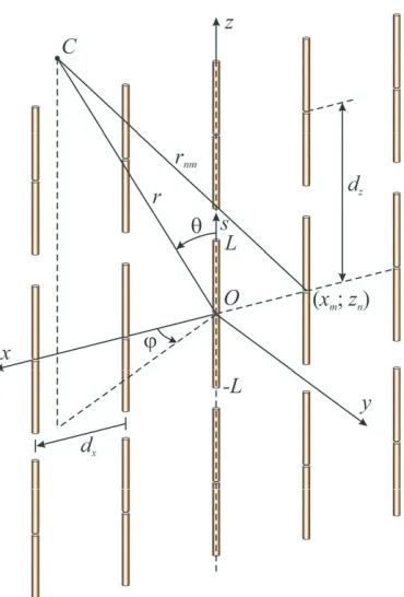
Cartesian coordinate system (x, y, z), whose origin coincides with the array center. The geometry of the array is shown in Fig. 1. Letdz be a distance between neighboring rows of vibrators, dx be a distance
Received 15 November 2017, Accepted 21 February 2018, Scheduled 25 February 2018
* Corresponding author: Mikhail V. Nesterenko ([email protected]).
Figure 1. The geometry of the antenna array.
between the centers of the vibrators in one row, Nz be the number of rows, andNx be the number of
vibrators in one row. We will also introduce a spherical coordinate system, whose polar axis coincides with axis {0z}, and the angle ϕis measured from axis{0x}.
We assume that all vibratorsN =Nz×Nxare of equal length 2Land are characterized by different
variable impedances ¯Znm(s), normalized to the wave impedance of the medium, Z0 =
μ1/ε1[Ohm],
and integer indicesn∈[1, Nz] andm∈[1, Nx]. We also assume that the vibrator radii satisfy thin-wire
approximations ρ2nmL 1 and ρnm
√ ε1μ1
λ 1, andλis the wavelength in free space. Let the vibrators be
excited by monochromatic voltage-delta generators with predetermined amplitudesVnm at the angular
frequency ω. If time dependency is specified in the form eiωt, an expression for longitudinal electric currents on vibrators can be written as [5]
Jnm(s) =− iωε1αVnm
2˜knmcos ˜knmL
sin ˜knm(L− |s|) =Jnmsin ˜knm(L− |s|), (1)
where ˜knm are the wave vectors averaged over the vibrator length, defined by the relation ˜knm2 (s) =
k12(1 +ki21αρnmnm ·21L L
−L
¯
Znm(s)ds); Jnm are the complex amplitudes of the vibrator currents; αnm =
1
2 ln[ρnm/(2L)] are natural small parameters; k1 = k √
ε1μ1, k = ω/c are the wave numbers; c ≈
2.998·1010cm/s is the light velocity in vacuum. Taking into account Equation (1), we can write the main electric field component of the vibrator radiation with indices (n, m) in the wave zone as
Enmθ =
60πi λ ·
e−ik1rnm
rnm
sinθ
L
−L
Jnm(s)e−ik1s
cosθ
ds
= 120πi λ ·
e−ik1rnm
rnm Jnm
cos (k1Lcosθ)−cos
˜ knmL
˜ k2
nm−(k1cosθ)2
˜
Since the far-field components Eϕ and Er of the array are equal to zeros, the total radiation field of
the array under condition that all vibrators are resonantly tuned by selecting intrinsic resistance of the δ-generators to compensate mutual influence of the vibrators can be presented as the sum of the radiation fields induced by each vibrator in the observation point C(r, θ, ϕ) as follows
Eθ(r, θ, ϕ) =
120πi λ
Nz
n=1
Nx
m=1
e−ik1rnm
rnm Jnm
cos (k1Lcosθ)−cos
˜ knmL
˜ k2
nm−(k1cosθ)2
˜
knmsinθ. (3)
Thus, the impedance synthesis problem is reduced to finding impedances ¯Znm(s) of each vibrator
using Equation (3) that can steer the radiation maximum (θmax, ϕmax) to the predefined direction in
space.
3. PROBLEM SOLUTION
First, let us represent expression (2) for the radiation field of an isolated vibrator as
Enmθ =
e−ik1rnm
rnm ·
60Jnm
√
ε1μ1sinθ
iF c(θ) +αnmβ¯nm F c(θ)
1 + cos2θ
sin2θ −k1Lsin (k1L)
, (4)
where F c(θ) = cos(k1Lcosθ) −cos(k1L) and ¯βnm = 2Lk11ρnm L
−L
¯
Znm(s)ds. Expression (4) is more
convenient for further analysis, since the first term in square brackets determines the RP of an isolated perfectly conducting vibrator, while the second term defines variation of the vibrator field due to its impedance coating.
The expression for the fieldEθ(r, θ, ϕ) in the wave zone can be presented in the following form
Eθ(θ, ϕ) = e−i(Nz+1)u/2e−i(Nx+1)v/2
60iF c(θ)
√
ε1μ1sinθ
×
Nz
n=1
Nx
m=1
Jnm
1−iαnmβ¯nm
1 + cos2θ sin2θ −
k1Lsin (k1L)
F c(θ)
ei(nu+mv), (5)
where u = k1dzcosθ and ν = k1dxsinθcosϕ. This formula is derived taking into account the
expression (4) and a difference of geometric paths from neighboring vibrators to the observation point C(r, θ, ϕ). If the vibrators are perfectly conducting, and all vibrator currents are equal, Jnm = J0,
expression (5) is simplified to
Eθ(θ, ϕ) =e−i(Nz+1)u/2e−i(Nx+1)v/2
60iF c(θ)J0 √
ε1μ1sinθ
Nz
n=1
einu
Nx
m=1
eimv. (6)
This expression includes two multiplayers in the form of independent power series, which represent the RPs with maxima directed along the axes{0z}and {0x}, respectively. One can see that the maximum of the RP is achieved if u=v= 0, and it is directed along axis {0y}, i.e., when θ=π/2 andϕ=π/2.
As known from the general theory of antenna arrays (see, e.g., [6]), a linear phase shift between currents of the array radiators results in radiation pattern steering. If the phase shifts between neighboring vibrators in the row and between adjacent rows are −Δu and −Δv, the direction of maximum array radiation (θmax;ϕmax) can be determined by the following relations
cosθmax= Δu/k1dz and sinθmaxcosϕmax= Δv/k1dx. (7)
Then, expression (6) can be represented as
Eθ(θ, ϕ) =e−i(Nz+1)u/2e−i(Nx+1)v/2
60iF c(θ)J0 √
ε1μ1sinθ
Nz
n=1
Nx
m=1
Expressions (5) and (8) become identical if the relations
1−e−ik1[(n−1)dzcosθ+(m−1)dxsinθcosϕ]=iαnmβ¯nm
1 + cos2θ sin2θ −
k1Lsin (k1L)
F c(θ)
θ=θmax;ϕ=ϕmax
(9)
are valid for any nand m.
In essence, the relations in Eq. (9) for given angles (θmax;ϕmax) can be interpreted as equations,
whose solution defines the matrix of unknowns{β¯nm}. It is easy to see that formula (9) for the 1D array
(at k1 =k, dz = 0, dx = d, m =n, αnm = α, ¯βnm = ¯βn) can be reduced to the expression obtained
in [5]: e−i(n−1)kdsinθcosϕ= [1−iαβ¯
n(1+cos
2θ sin2θ −
kLsin(kL)
F c(θ) )]
θ=θmax;ϕ=ϕmax
.
Without loss of generality, let us assume that all vibrators have different complex impedances ¯
Znm = ¯Rnm+iX¯nm, constant along the longitudinal axes of the vibrators. Then Equation (9) can be
represented in the following form
1−e−ik1γnm =iα nm
¯
Rnm+iX¯nm
k1ρnm
1 + cos2θmax
sin2θmax
−k1Lsin (k1L)
F c(θmax)
, (10)
whereγnm= [(n−1)dzcosθmax+ (m−1)dxsinθmaxcosϕmax].
Since parametersαnm for lossless media are real, the final formula for the real and imaginary parts
of vibrator surface impedances can be written using Eq. (10) as
¯
Rnm = k1ρnm
sin (k1γnm)
αnm
1 + cos2θmax
sin2θmax
−k1Lsin (k1L)
F c(θmax)
;
¯
Xnm= −k1ρnm
[1−cos (k1γnm)]
αnm
1 + cos2θmax
sin2θmax
−k1Lsin (k1L)
F c(θmax)
.
n= 1,2, . . . , Nx; m= 1,2, . . . , Ny; (11)
Formulas (9) and (11) remain valid for arbitrary number of vibrators in the array and arbitrary distances between the vibrators.
4. NUMERICAL RESULTS
As an example, consider a 2D array of symmetrical half-wave impedance vibrators radiating in the front half-space 0 ≤θ ≤ π, 0 ≤ ϕ≤ π (Fig. 1). The number of array elements is 25(Nx = 5, Nz = 5), and
0.0 0.2 0.4 0.6 0.8 1.0 90° 80° 70° 60° 50° 100° 110° 120° 130° (a) (b)
0 30 60 90 120 150 180
o
ϕ 0 30 60 90o 120 150 180
θ | E ( θ , ϕ )| / | E ( θ , ϕ )| θ max max θ max | E ( θ , ϕ )| / | E ( θ , ϕ )| θ max max θ max 0.0 0.2 0.4 0.6 0.8 1.0
θ max= ϕ max= θ max= ϕ max=
90° 80° 70° 60° 50° 100° 110° 120° 130°
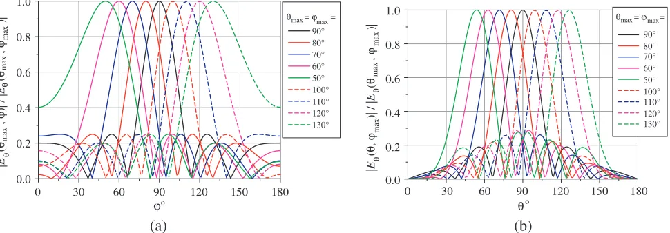
Figure 2. Normalized radiation patterns of the array with array periodsdx= 0.5λ,dz = 0.5λ: (a) the
0.0 0.2 0.4 0.6 0.8 1.0
(a) (b)
0 30 60 90 120 150 180
o
ϕ 0 30 60 90o 120 150 180
θ
|
E
(
θ
,
ϕ
)| / |
E
(
θ
,
ϕ
)|
θ
max
max
θ
max
|
E
(
θ
,
ϕ
)| / |
E
(
θ
,
ϕ
)|
θ
max
max
θ
max
0.0 0.2 0.4 0.6 0.8 1.0
90° 80° 70° 60° 50° 100° 110° 120° 130°
θ max= ϕ max=
90° 80° 70° 60° 50° 100° 110° 120° 130°
θ max= ϕ max=
Figure 3. Normalized radiation patterns of the array with periodsdx = 0.25λ,dz= 0.5λ: (a) the angle
θmaxis fixed, (b) the angle ϕmax is fixed.
20 40 60 80 100 120 140 160 180
20 40 60 80 100 120 140 160 180
0.0 0.1 0.2 0.3 0.4 0.5 0.6 0.7 0.8 0.9
(a) (b)
o ϕ
o
θ
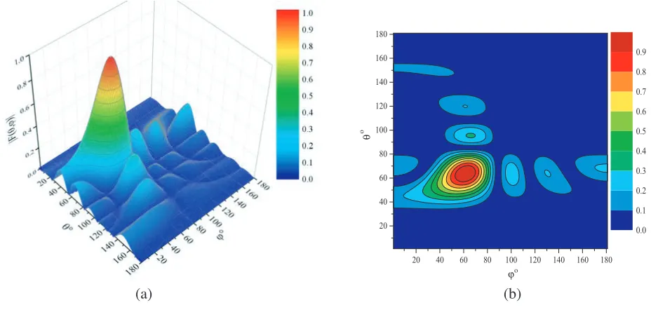
Figure 4. The 3D radiation pattern of the antenna array with parameters: dz = dx = 0.5λ,
θmax=ϕmax= 60◦: (a) surface plot, (b) contour plot.
the vibrator length and radius are L = λ/4 and ρnm = L/75. The problem consists in finding the
impedances in Eq. (11) of each vibrator such that the main lobe of the RP is oriented in a predefined direction (θmax;ϕmax).
The results of numerical simulations are presented for two arrays with different geometric structures (dx = 0.5λ, dz = 0.5λ and dx = 0.25λ, dz = 0.5λ) are shown in Fig. 2 and Fig. 3, where variations of
angle (θmax;ϕmax) are shown symmetrically with respect to direction (θ= 90◦;ϕ= 90◦) corresponding
to main lobe orientation for the array with perfectly conducting vibrators.
As can be seen from the figures, the simulation results confirm the possibility to vary the direction of the array RP maximum within the entire half-space, at least theoretically, by varying the intrinsic impedances of the vibrators. As expected, the main lobe width depends on array aperture dimensions as seen from the observation angles, and therefore slightly varies during spatial scanning. As an example, Fig. 4 shows the surface and contour plots of RP of the antenna array.
Table 1. Calculated impedances for the RP shown in Fig. 4.
¯
Rnm X¯nm
0 0.37 0.155 −0.305 −0.282 0 −0.299 −0.724 −0.602 −0.126 0.378 0.079 −0.345 −0.223 0.252 −0.378 −0.748 −0.533 −0.073 −0.096 0 −0.37 −0.155 0.305 0.282 −0.757 −0.457 −0.033 −0.155 −0.63
−0.378 −0.079 0.345 0.223 −0.252 −0.378 −0.008 −0.224 −0.684 −0.66 0 0.37 0.155 −0.305 −0.282 0 −0.299 −0.724 −0.602 −0.126
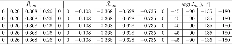
Table 2. Calculated values of the impedances.
¯
Rnm X¯nm arg(Jnm),[◦]
0 0.26 0.368 0.26 0 0 −0.108 −0.368 −0.628 −0.735 0 −45 −90 −135 −180 0 0.26 0.368 0.26 0 0 −0.108 −0.368 −0.628 −0.735 0 −45 −90 −135 −180 0 0.26 0.368 0.26 0 0 −0.108 −0.368 −0.628 −0.735 0 −45 −90 −135 −180 0 0.26 0.368 0.26 0 0 −0.108 −0.368 −0.628 −0.735 0 −45 −90 −135 −180 0 0.26 0.368 0.26 0 0 −0.108 −0.368 −0.628 −0.735 0 −45 −90 −135 −180
of vibrators in the array and arbitrary distance between vibrators. However, in a general case, the impedances ¯Znm = ¯Rnm+iX¯nm (11), thus calculated, cannot guarantee that the inequality ¯Rnm ≥0,
arising from energy considerations, holds. Such a situation can be observed in Table 1, where the real and imaginary parts of the vibrator impedances calculated for the RP in Fig. 4 are shown.
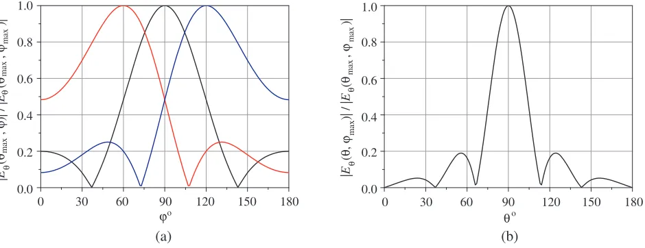
The normalized RPs of the array (dx = 0.25λ, dz = 0.5λ) are represented in main planes in Fig. 5.
The simulation results show that the real parts of the impedances remain positive if angle θmax= 90◦
and angle ϕmax varies at the interval ϕmax ∈ [60◦,120◦]. As an example, calculated impedances are
given in Table 2 for angles θmax = 90◦ and ϕmax = 60◦. As can be seen from the table, all positive
values are observed in the case when the resulting difference in the phase currents of extreme radiators in the lattice does not exceed 180◦. If ¯Rnm<0, the real part of impedances ¯Rnm should be interpreted
as effective physical quantities [7], which can be realized only as a result of electrodynamic interactions between the vibrators and additional scatterers. Impedances ¯Znm with the real parts ¯Rnm ≥0 which
can be interpreted as traditional intrinsic impedances under conditions that the individual vibrators can be manufactured in the form of cylindrical structures with complex intrinsic structures [4]. Therefore, for practical applications, limiting scanning angles of the array RP should be determined for which the condition ¯Rnm≥0 is satisfied. From the point of view of physical interpretation, such studies can most
obviously be carried out if the RP is scanned only in one plane.
The normalized RPs of array (dx= 0.25λ,dz = 0.5λ) are represented in main planes in Fig. 5. The
simulation results show that the real parts of the impedances remain positive if angle θmax = 90◦ and
angle ϕmax varies at the interval ϕmax ∈ [60◦,120◦]. As an example, calculated impedances are given
in Table 2 for angles θmax = 90◦ and ϕmax = 60◦. As can be seen from the table, all positive values
are observed in the case when the resulting difference in the phase currents of the extreme radiators in the lattice does not exceed 180◦. As can be seen from Table 2, positive ¯Rnm are observed if in the
phase shifts of the currents on the edge vibrators arg(Jnm) do not exceed 180◦. The simulation results
have also shown that this condition is valid for other array geometries, particularly for two-dimensional scanning.
The maximum angle of the RP deviation relative to the normal Δϕmax = 90◦ −ϕmax for ¯Rnm
to remain positive can be estimated by Δϕmax = ±arcsin(kdx(Nπx−1)) = ±arcsin(2dx(Nλx−1)) or by
Δϕmax≈ ±2dx(Nλx−1) ·180 ◦
π valid for small deviations. This estimate relative to the main lobe width at
0.0 0.2 0.4 0.6 0.8 1.0
(a) (b)
0 30 60 90 120 150 180
o
ϕ 0 30 60 90θo 120 150 180
|
E
(
θ
,
ϕ
)| / |
E
(
θ
,
ϕ
)|
θ
max
max
θ
max
|
E
(
θ
,
ϕ
)| / |
E
(
θ
,
ϕ
)|
θ
max
max
θ
max
0.0 0.2 0.4 0.6 0.8 1.0
Figure 5. RPs in the main planes.
5. CONCLUSION
The method of impedance synthesis of the radiation pattern, proposed in [5] for linear vibrator structures, is generalized for the 2D vibrator arrays. The problem of impedance synthesis for the double periodic arrays is solved analytically. The derived formulas allow defining the impedance of each vibrators that permit to steer the RP maximum in a predefined direction. The formulas can be used to develop algorithms for controlling antenna arrays, for example, for spatial scanning of the RP. The approach is characterized by using the variable vibrator impedance as the averaged integral coefficient. This methodology turns out to be common for the radiators with impedance coatings of various types. The method validity is confirmed by reduction of the obtained formulas for particular cases of 1D equidistant arrays. The numerical simulation of the 2D antenna array consisting of 25(N = 25, Nx = 5, Nz = 5) symmetrical half-wave vibrators (L=λ/4) has been carried out,
which confirms a possibility to scan the antenna RP in the front half-space by varying complex internal impedances of the vibrators. The physical realization of this possibility is analyzed. The results obtained in the article can be used for modeling of adaptive antenna arrays with adjustable dynamic variation of parameters and characteristics depending upon influence of external or intrinsic factors.
REFERENCES
1. Bakhrakh, L. D. and S. D. Kremenetsky, Synthesis of Radiation Systems (Theory and Methods of Calculation), Sov. Radio, Moscow, 1974 (in Russian).
2. Skobelev, S. P.,Phased Array Antennas with Optimized Element Patterns, Artech House, Boston, 2011.
3. Berdnik, S. L., V. A. Katrich, M. V. Nesterenko, and Y. M. Penkin, “Electromagnetic waves radiation by a vibrators system with variable surface impedance,” Progress In Electromagnetics Research M, Vol. 51, 157–163, 2016.
4. Nesterenko, M. V., V. A. Katrich, Yu. M. Penkin, V. M. Dakhov, and S. L. Berdnik,Thin Impedance Vibrators. Theory and Applications, Springer Science+Business Media, New York, 2011.
5. Penkin, Yu. M., V. A. Katrich, and M. V. Nesterenko, “Formation of radiation fields of linear vibrator arrays by using impedance synthesis,” Progress In Electromagnetics Research M, Vol. 57, 1–10, 2017.
6. Amitay, N. V. Galindo, and C. P. Wu,Theory and Analysis of Phased Array Antennas, John Wiley & Sons Inc, New York, 1972.