Backscattering from Electrically Large Target above Nonlinear
Sea Surface
Wei Luo1, *, Yuqi Yang2, and Honggang Hao1
Abstract—The composite scattering of an electrically large target above nonlinear sea surface is analyzed based on the reciprocity theorem. The two-dimensional nonlinear sea surface is simulated with the Fast Fourier transform (FFT), with which the phase modified two-scale method is utilized to calculate the scattering field of the wind-driven sea surface. The electromagnetic currents of the sea surface, which are excited with plane wave, are calculated with the iterated Kirchhoff approximation (KA). The coupling scattering between the target and the sea surface, which includes the complex scattering matrix of composite scattering, is ingeniously reduced to the integrals involving the target scattering and high order currents of sea surface. A sensitivity analysis is performed for the dependency of the coupling scattering on the target features. The relationship of the full composite scattering model with the sea state is examined, which provides theoretical basis for the target recognition.
1. INTRODUCTION
The composite electromagnetic scattering from an electrically large target in the sea background is of great significance for target recognition, sea surveillance, and radar image technology [1–3]. Although many numeric methods have been developed for the modeling of sea surface scattering for decades, the modulation relationship between radio wave and dynamic sea surface has not been completely realized. Due to the contradiction between the accuracy and efficiency of calculation, the research of target electromagnetic signature in sea background remains a significant issue to be solved urgently [4].
The sea clutter is seriously influenced by the multiple scattering caused by the sea surface fluctuation. A second-order received power model is developed for the case of mixed-path ionosphere-ocean propagation with Fast Fourier Transform [5]. It has been proved that the interactions between the internal waves of wind driven sea surface lead to nonlinear dynamics characteristic [6]. The microwave scattering from two-dimensional wind fetch-limited near shore sea surface is investigated with the second-order small-slope approximation (SSA-II). Monostatic and bistatic numerical results both indicate that the nonlinear interaction among waves has a greater impact on NRCS for co-polarizations than their cross-polarized counterparts [7–9].
In order to extend the solutions of rough surface scattering problem, some integral equation methods are promoted to improve the calculation efficiency [10]. The boundary integral equation (BIE) method is used to solve jointly the scattering problem from the sea surface and the propagation problem by including the Green’s function. The linear system obtained from the method of moments (MOM) by discretizing the integral equations is efficiently solved with the forward-backward method (FBM) [11]. An advanced integral equation model is also presented by giving its general framework of model developments, model expressions, and predictions of bistatic scattering for various surface parameters [12].
Received 21 May 2017, Accepted 17 June 2017, Scheduled 6 July 2017
* Corresponding author: Wei Luo ([email protected]).
1 College of Electronic Engineering, Chongqing University of Posts and Telecommunications, Chongqing, China. 2 Electronic
Interests on the coupling effects in the composite scattering have been aroused recently. The improved algorithms based on MOM, such as The Generalized Forward-Backward Method (GFBM) and e Mode-Expansion Method [13, 14], are utilized to evaluate the composite scattering for the unified geometric model of the surface and the target. An efficient multi-region hybrid method of the finite element method (FEM) combined with the boundary integral method (FEM-BIM) is also proposed for the fast simulation of composite scattering. Mutual coupling between different subordinate regions is approximately considered by field integral equations based on KA. Since FEM and BIM are only performed on the target and the dominant region of the sea, the number of unknowns is dramatically reduced [15]. A fast far-field approximation (FAFFA) is also applied to speed up the mutual interactions between the targets and the sea surface, and improved iteration method is proposed to reduce the convergence steps for the MLFMA process [16].
Based on the reciprocity theorem, this paper investigates the composite scattering of an electrically large target on the two-dimensional randomly rough sea surface. The phase modified two-scale method (MTSM) and the method of equivalent currents (MEC) are applied to evaluate the backscattering of the sea surface and the targets, respectively. The coupling scattering between the target and sea surface is calculated with the high order iterated Kirchhoff approximation (KA) currents. The pertinent results and discussion on the effects of the coupling field are presented.
2. NONLINEAR SEA SURFACE
Neglecting the interaction of the harmonics of the sea spectrum ψ(K, ϕ), the linear surface can be assumed as a superposition of harmonics of which amplitudes are independent Gaussian random variables with variances proportional to certain spectrum components. With the help of inverse Fast Fourier transform (IFFT), the linear height fluctuation ζ(r, t) is obtained by the filtered sea spectrum
ζ(r, t) = 1
LxLyF
I[F(K
x, Ky)] (1)
where the size of the sea surface is denoted withLx and Ly, and the complex amplitude is given as
F(Kx, Ky) =γ2π
LxLyψ(Kx, Ky) exp (jωt) (2)
γ is a complex Gaussian process with zero mean and unity standard deviation, andψ(Kx, Ky) is the sea spectrum. ωis the angular frequency of sea spectrum. This paper considered the 2-D Pierson-Moskowitz spectrum
ψ(K, ϕ) = α 2K4 exp
− βg2
K2U4
cos4
ϕ−ϕω
2
(3)
whereα andβ are constants, and U is the wind speed at a height of 19.5 m. K is the wave number of the sea wave.
Due to the interactions of the harmonics, the assumption of the linear model is no longer valid in high frequency bands. Based on the hydrodynamic equations, the one-dimensional nonlinear surface is derived as the Hilbert transform of the linear surface [17]. The vector Hilbert transform is expressed as
ht(r) = Re
K
−jK K
F(K) exp (jKr). (4)
Equation (4) is transformed to the frequency domain as
Ct(K) = 1 N
r
exp [jKht(r)]−1
K exp (−jKr) (5)
Since Equation (5) cannot be calculated by Fast Fourier transform (FFT), it is approximately written as
Ctn(K) = 1 N
r
[jKht(r)]n
It can be proved that the first order of Equation (6) is equivalent to the linear term F(K). Then the second-order approximation of the Creamer model written as the modified representation of Equation (1)
ζ(r, t) = 1
LxLyF
IF(K
x, Ky) +Ct2 (7)
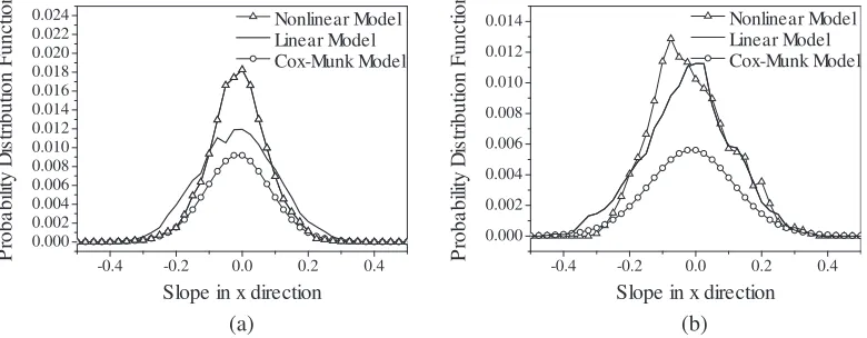
The Bragg scattering from the sea surface is modulated by the tilted sea surface slope. Based on the measurements, Cox and Munk found that the probability density of the sea surface slopes can be well described by the Gram Charlier distribution. Thus the Cox-Munk model is widely used to evaluate the sea wave fluctuation and calculate the electromagnetic scattering of sea surface [18]. The slopes probability distribution functions (PDF) of the simulated linear surface and the nonlinear surface are compared with the Cox-Munk model in Figure 1. It is observed that the discrepancy of the linear and nonlinear models is more apparent in low wind speed than the one in the high wind speed.
-0.4 -0.2 0.0 0.2 0.4 0.000
0.002 0.004 0.006 0.008 0.010 0.012 0.014 0.016 0.018 0.020 0.022 0.024
P
ro
b
a
b
ilit
y Dis
tr
ib
u
tio
n
F
u
n
ct
io
n
Slope in x direction
Nonlinear Model Linear Model Cox-Munk Model
-0.4 -0.2 0.0 0.2 0.4 0.000
0.002 0.004 0.006 0.008 0.010 0.012 0.014
P
ro
b
a
b
ilit
y Dis
tr
ib
u
tio
n
F
u
n
ct
io
n
Slope in x direction
Nonlinear Model Linear Model Cox-Munk Model
(a) (b)
Figure 1. Probability distribution function of surface slope in x direction. (a) U19.5 = 10 m/s. (b) U19.5 = 20 m/s.
3. COMPOSITE SCATTERING MODEL
3.1. Reciprocity Theorem
The reciprocity theorem has been used to analyse the scattering from the targets above the slightly rough surface [19]. This paper extends this idea to the composite scattering from the electrically large targets above the sea surface.
According to the reciprocity of scatters, the composite scattering of the targets on the sea surface are expressed as
ˆ
p·EJ1 =
S1
J1·EeddS+
S1
J1·Ee2cdS (8)
ˆ
p·EJ2 =
S2
J2·EeddS+
S2
J2·Ee1cdS (9)
J1 andJ2 are the electrical currents on the sea surface and the target, respectively. Ee2c and Ee1c are the interactive incident waves between the sea surface and the target. Eed is the electrical field induced by the point electrical source in the far zone
Eed(r) =E0exp(−jks·r)ˆp
E0 =
jkZ0
4πR0
exp(jkR0)
Z0 is the characteristic impedance, and pˆ is the polarization direction of the electrical field. Other parameters can be found in reference [19].
The integrals of J1 and J2 with the incidence wave Eed are the direct scattering from the sea surface and target, and the second integral terms in Equations (8) and (9) are the coupling scattering field between the surface and target
Es =
S1
J1·EeddS (11)
Et =
S2
J2·EeddS (12)
Ere =
S2
J2·Ee1cdS+
S1
J1·Ee2cdS (13)
EsandEtare the direct scattering fields of the sea surface and target respectively, andEreis the coupling scattering field between the surface and target. Due to the complex distribution of the currents on the target, the first integral in Equation (13) is more complicated than the second one. However, it is proved that the two terms are equivalent to each other for the backscatter case. Thus Equation (13) is rewritten as
Ere = 2
S1
J1·Ee2cdS (14)
It is obvious that the summation of the components is the total composite scattering
Etotal =Es+Et+Ere (15)
In the following sections, the integrals in Equations (11) and (12) are calculated with the MEC and phase-modified TSM, and the coupling scatteringEre is evaluated with the iterated KA currents.
3.2. Direct Scattering of Target and Sea Surface
The MEC is based on the fact that a limited result can be obtained by the radiation integral of scattering field of any limited distribution of currents in far zone. The equivalent currents are assumed to exist on the edge of the loop, and the target scattering field is expressed as [20]
Et=jk
c
Z0I
rkˆs×(ˆks׈t) +Mr kˆs׈t
exp(−jkR
0) 4πR0
dl (16)
It can be seen that the choice of reasonable equivalent edge currents (I and M) is very significant for the accuracy of calculation. The GTD equivalent edge current (GTDEEC) is used in this paper.
In the high frequency bands, the TSM is used for the calculation of sea surface scattering, which reckons that the waves contributing to the Bragg process are locally tilted by large-scale waves. The classical scattering coefficient of sea surface is formulated as
σpq0 (θi) =
∞
−∞ ∞
−cotθi
σpqSP M(θi) (1 +zxtanθi)
P(zx, zy) dzxdzy
(17)
σpqSP M(θi) is the SPM solution to the scattering from the small scale, andP(zx, zy) is the slope probability density function as viewed from the incidence direction.
Since the nonlinear sea surface model is discretized with triangular facets in this paper, the integral on the surface is replaced with the summation and Equation (17) rewrites as
σpq0 (θi) =
1 M
1 N
M
m=1
N
n=1
σpqSP M(θi)
[1 +zx(xm, yn) tanθi]
Considering the phase shift of each scattering facet, the classical TSM is modified with the modified facet phase. The facets should be large enough for the electromagnetic wavelength, and be small enough to characterize the phase variation of the surface fluctuation. With the additional phase, the scattering field of sea surface is obtained with phase-modified TSM
Epqs = 1
M 1 N
M
i=1
N
j=1
IijΔSexp (jφadd) (19)
Iij = σpqSP M(θi) [1 +zx(xm, yn) tanθi] (20)
φadd = ξ·ϕmax+ (ki−ks)·r (21)
Iij and ΔS are the scattering intensity and area of single facet respectively. ϕmax is the maximum of the phase difference in the facet, andξ is a random number (ξ ∈ [−1/2,1/2]). r is the location of the facet in the global reference frame and (ki−ks)·ris the phase delay caused by the relative position of the facets.
3.3. Coupling Scattering Evaluated by High Order Surface Currents
According to Equation (13), the accuracy of the calculation of coupling field depends on the electromagnetic currents of the sea surface. This paper introduces the iterated KA electromagnetic currents to improve the calculation accuracy [21]
Jn=J0+ ˆn×Hcn(1 +Rv,h) Mn=M0−nˆ×Ecn(1 +Rv,h)
n= 1,2, . . . , N
(22)
whereJ0 andM0are the KA electromagnetic currents. JnandMnare iterative solutions of the surface currents, while n denotes the order of the iteration. Rv,h is the local reflection coefficient of the sea surface. AndEcn and Hcn are given as
Ecnr,r=
S
−jωμJn−1
rGr,r− Mn−1
r× ∇Gr,r dS
Hcnr,r=
S
−jωεMn−1
rGr,r+ Jn−1
r× ∇Gr,r dS
(23)
G(r,r) is the Green Function in the free space. Equation (23) is deduced from the Stratton-Chu equations, which accounts for the multiple scattering between different parts of the sea surface. It is evident that the increase of currents order will lead to the improvement of calculation accuracy.
By substitution of Equation (22) into Equation (14), the coupling scattering fieldEre is efficiently calculated. Then the radar cross section (RCS) of the total composite scattering is calculated
RCS = 4π lim R→∞R
2
Etotal2
|Einc|2 (24)
4. NUMERICAL RESULTS
The accuracy of the modified TSM is evaluated with measurement data from radar surveillance [22]. Figure 2 shows the backscattering coefficient varied with the wind speed. The frequency of the incidence radio wave is 14 GHz, and coefficients are HH polarized. It is shown that the scattering intensity increases with the wind speed, and decreases with the incidence angle. Moreover, the scattering intensity of the upwind is stronger than the one of crosswind. The numerical results of the modified TSM agree with the measured data well.
In Figure 3(a), the height of the cube (distance from the sea surface to the cube) keeps 10 m, and the length of the cube varies from 1m to 10 m. It is observed that the coupling scattering intensity increases with the size of the cube. While the variation of the monobistatic RCS is gentle in small incidence angles, the oscillation is found in large incidence angles. It is concluded that the distribution of the random fluctuation of the sea surface on the coupling scattering is enhanced by the increasing incidence angles. In Figure 3(b), the height of the cube varies from 10 m to 20 m, and the cube size keeps constant. While the coupling scattering is apparently weaken by the distance between the sea surface and the cube in the moderate incidence angles, the strong oscillations of the numerical results are found in the large incidence angles.
Based on the reciprocity theorem, the total composite scattering of the cone-cylinder model above
4 6 8 10 12 14 16
-45 -40 -35 -30 -25 -20 -15 -10 -5 0 B ack sc at te ri ng C oef fi ci en t ( dB )
Wind Speed (m/s)
Measured data 30
o
Modified TSM 30
o
Measured data 40
o
Modified TSM 40
o
Measured data 50
o
Modified TSM 50
o
4 6 8 10 12 14 16
-45 -40 -35 -30 -25 -20 -15 -10 -5
Measured data 30o Modified TSM 30
o
Measured data 40o
Modified TSM 40
o
Measured data 50o Modified TSM 50
o B ack sc at te ri ng C oef fi ci en t ( dB )
Wind Speed (m/s)
(a) (b)
Figure 2. Comparison of the modified TSM and measured data in different wind direction. (a) Upwind. (b) Crosswind.
1 2 3 4 5 6 7 8 9 10
-30 -20 -10 0 10 20 30 40 50 M onos ta ti c R C S ( dB sm ) Length (m) θi=9 o
θi=29
o
θi=45
o
θi=69
o
10 11 12 13 14 15 16 17 18 19 20 -20 -15 -10 -5 0 5 10 15 20 25 M onos ta ti c R C S ( dB sm ) Height (m)
θi=45
o
θi=55
o
θi=62
o
θi=70
o
(a) (b)
Figure 3. Monostatic RCS of coupling scattering varied with the (a) length and (b) height of the cube.
15 m 2 m
6 m
-80 -60 -40 -20 0 20 40 60 80 -30
-20 -10 0 10 20 30 40 50
Target Scattering Coupling Scattering
Target Scattering Coupling Scattering
M
onos
ta
ti
c R
C
S
(
dB
sm
)
Incidence Angle (deg) Sea Scattering Composite Scattering Target Scattering
-80 -60 -40 -20 0 20 40 60 80 -10
0 10 20 30 40 50 60
M
onos
ta
ti
c R
C
S
(
dB
sm
)
Incidence Angle (deg) Wind Speed=15 m/s Wind Speed=10 m/s Wind Speed=5 m/s
(a) (b)
Figure 5. Composite scattering varies with the incidence angle. (a) Components of the composite
scattering. (b) Influence of the wind speed on the composite scattering.
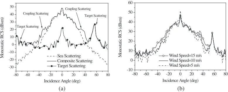
the sea surface is analyzed. The size of the cone-cylinder is shown in Figure 4, and the incidence wave is 3 GHz. Figure 5(a) shows the components of the composite scattering and the influences of the target and the coupling scattering on the total scattering. Although the sea scattering is dominant in the small incidence angles, the peaks of the monostatic RCS is caused by the increased coupling scattering in the moderate incidence angles. The backscattering of the target is much stronger than the one of the sea surface, and lead to the apparent peak in the incidence angle 55◦. Figure 5(b) shows the impact of the sea state on the composite scattering. Due to the dominance of the specular scattering from the sea surface, the peak decrease with the wind speed in normal incidence direction. With the increment of the incidence angle, the influence of sea surface roughness on the scattering is enhanced. Thus the monostatic RCS of composite scattering increases with wind speed. It is noted that the peak at the incidence angle 55◦ is independent with sea state, which is caused by the target scattering.
Since the reciprocity theorem and iterated Kirchhoff approximation currents are introduced in this paper, the requirement on computer memory is reduced to 200 Mbytes for each composite scattering model. The CPU time of composite scattering calculation is shown in Table 1, whereN is the order of electromagnetic currents and U is the wind speed. The numerical analysis can be realized on general computers.
Table 1. CPU time of composite scattering calculation.
U = 5 m/s U = 10 m/s U = 15 m/s
N = 0 120 s 220 s 345 s
N = 1 213 s 410 s 531 s
N = 2 996 s 1352 s 1521 s
5. CONCLUSIONS
The composite electromagnetic scattering of the electrically large target above the nonlinear sea surface is analyzed based on the reciprocity theorem. The electromagnetic interaction of the sea surface and the target is evaluated in different conditions. While the high order iterated KA currents improve calculation accuracy of mutual coupling field based on the integral in Equation (14), the nonlinear surface model provides realistic sea surface sample for the electromagnetic scattering research.
the target and the sea surface. According to the simulation of the composite scattering, the sea surface scattering is dominant in the normal incidence direction, and the scattering contribution from the target is much stronger than the one of sea surface in the large incidence angles. Moreover, the influence of coupling scattering is observed in the moderate incidence angles. The conclusions provide theoretical analysis for the target recognition from the sea clutter and radar imaging of composite scattering.
ACKNOWLEDGMENT
The authors would like to thank the anonymous reviewers for their invaluable comments and suggestions, which lead to great improvement of our manuscript, and also thank the National Natural Science Foundation of China under Grant No. 41606203. This work is supported by the Science and Technology Research Program of Chongqing Municipal Education Commission (Grant No. KJ1600421).
REFERENCES
1. Wu, Y. M. and W. C. Chew, “The modern high frequency methods for solving electromagnetic scattering problems,”Progress In Electromagnetics Research, Vol. 156, 63–82, 2016.
2. Wu, Z.-S., J.-J. Zhang, and L. Zhao, “Composite electromagnetic scattering from the plate target above a one-dimensional sea surface: Taking the diffraction into account,” Progress In
Electromagnetics Research, Vol. 92, 317–331, 2009.
3. Baussard, A., M. Rochdi, and A. Khenchaf, “PO/Mec-based scattering model for complex objects on a sea surface,” Progress In Electromagnetics Research, Vol. 111, 229–251, 2011.
4. Wang, R., L. X. Guo, and Z. B. Zhang, “Scattering from contaminated rough sea surface by iterative physical optics model,” IEEE Geoscience and Remote Sensing Letters, Vol. 13, No. 14, 500–504, 2016.
5. Chen, S. Y., E. W. Gill, and W. M. Huang, “A high-frequency surface wave radar ionospheric clutter model for mixed-path propagation with the second-order sea scattering,” IEEE Transactions on
Antennas and Propagation, Vol. 64, No. 12, 5373–5381, 2016.
6. Nouguier, F., S. T. Grilli, and C. A. Gu´erin, “Nonlinear ocean wave reconstruction algorithms based on simulated spatiotemporal data acquired by a flash LIDAR camera,” IEEE Transactions
on Geoscience and Remote Sensing, Vol. 52, No. 3, 1761–1771, 2014.
7. Nie, D., M. Zhang, and N. Li, “Investigation on microwave polarimetric scattering from two-dimensional wind fetch- and water depth-limited nearshore sea surfaces,” Progress In
Electromagnetics Research, Vol. 145, 251–261, 2014.
8. Li, X. F. and X. J. Xu, “Scattering and Doppler spectral analysis for two-dimensional linear and nonlinear sea surfaces,” IEEE Transactions on Geoscience and Remote Sensing, Vol. 49, No. 2, 603–611, 2011.
9. Yang, W., Z. Q. Zhao, C. H. Qi, and Z. P. Nie, “Electromagnetic modeling of breaking waves at low grazing angles with adaptive higher order hierarchical Legendre basis functions,” IEEE
Transactions on Geoscience and Remote Sensing, Vol. 49, No. 1, 346–352, 2011.
10. Luo, H. J., G. D. Yang, Y. H. Wang, J. C. Shi, and Y. Du, “Numerical studies of sea surface scattering with the GMRES-RP method,”IEEE Transactions on Geoscience and Remote Sensing, Vol. 5, No. 4, 2064–2073, 2014.
11. Bourlier, C., H. K. Li, and N. Pinel, “Low-grazing angle propagation and scattering above the sea surface in the presence of a duct jointly solved by boundary integral equations,”IEEE Transactions
on Antennas and Propagation, Vol. 63, No. 2, 667–677, 2015.
12. Chen, K.-L., K.-S. Chen, Z.-L. Li, and Y. Liu, “Extension and validation of an advanced integral equation model for bistatic scattering from rough surfaces,”Progress In Electromagnetics Research, Vol. 152, 59–76, 2015.
14. Zhang, Y., J. Lu, and J. Pacheco, “Mode-expansion method for calculating electromagnetic waves scattered by objects on rough ocean surfaces,” IEEE Transactions on Antennas and Propagation, Vol. 53, No. 5, 1631–1639, 2005.
15. Guo, L. X. and R. W. Xu, “An efficient multiregion FEM-BIM for composite scattering from an arbitrary dielectric target above dielectric rough sea surfaces,” IEEE Transactions on Geoscience
and Remote Sensing, Vol. 53, No. 7, 3885–3896, 2015.
16. Qi, C., Z. Zhao, and Z.-P. Nie, “Numerical approach on Doppler spectrum analysis for moving targets above a time-evolving sea surface,” Progress In Electromagnetics Research, Vol. 138, 351– 365, 2013.
17. Soriano, G., M. Joelson, and M. Saillard, “Doppler spectra from a two-dimensional ocean surface at L-Band,” IEEE Transactions on Geoscience and Remote Sensing, Vol. 44, 2430–2437, 2006. 18. Cox, C. and W. Munk, “Measurement of the roughness of the sea surface from photographs of the
sun glitter,” Journal of the Optical Society of America, Vol. 44, No. 11, 838–850, 1954.
19. Chiu, T. and K. Sarabandi, “Electromagnetic scattering interaction between a dielectric cylinder and a slightly rough surface,” IEEE Transactions on Antennas and Propagation, Vol. 47, No. 5, 902–912, 1999.
20. Zhang, M., W. Luo, G. Luo, C. Wang, and H.-C. Yin, “Composite scattering of ship on sea surface with breaking waves,” Progress In Electromagnetics Research, Vol. 123, 263–277, 2012.
21. Luo, W., M. Zhang, P. Zhou, and H. C. Yin, “Analysis of multiple scattering from two-dimensional dielectric sea surface with iterative Kirchhoff approximation,” Chinese Physics B, Vol. 19, No. 8, 379–383, 2010.
22. Schroeder, L. C., D. H. Boggs, and G. Dome, “The relationship between wind vector and normalized radar cross section used to derive SEASAT-A satellite scatterometer winds,”Journal of Geophysical