Impact of Extremely Low-Frequency Magnetic Fields on Human Postural Control

(1)

Western University Western University

Scholarship@Western

Electronic Thesis and Dissertation Repository

11-14-2016 12:00 AM

Impact of Extremely Low-Frequency Magnetic Fields on Human

Postural Control

Alicia N. Allen

The University of Western Ontario Supervisor

Dr. Alexandre Legros

The University of Western Ontario

Graduate Program in Kinesiology

A thesis submitted in partial fulfillment of the requirements for the degree in Master of Science © Alicia N. Allen 2016

Follow this and additional works at: https://ir.lib.uwo.ca/etd Part of the Other Kinesiology Commons

Recommended Citation Recommended Citation

Allen, Alicia N., "Impact of Extremely Low-Frequency Magnetic Fields on Human Postural Control" (2016). Electronic Thesis and Dissertation Repository. 4341.

https://ir.lib.uwo.ca/etd/4341

This Dissertation/Thesis is brought to you for free and open access by Scholarship@Western. It has been accepted for inclusion in Electronic Thesis and Dissertation Repository by an authorized administrator of

(2)

Abstract

The general public and workers can be exposed to high-levels of power-line frequency magnetic fields (MFs - up to 10 mT). Although such time-varying MFs have the potential to modulate human postural control, no existing studies have explored MF exposure levels that possibly trigger acute sway responses. This work evaluates time-varying MF exposure (up to 100 mT) in the extremely low frequency range (ELF – up to 300 Hz) and its effects on human postural control. Twenty-two healthy participants were each exposed to randomized, 5-second MF and electric stimulations (0, 50 and 100 mT and 1.5 mA respectively) given at different frequencies (20, 60, 90, 120, and 160 Hz). A force-plate collected participant Center Of Pressure (COP) displacement. Results revealed sway modulations resulting from electric stimulations but not from MF exposures. The mechanical stabilization induced by the inertia of the head-mounted exposure system might have masked acute sway responses.

Keywords

(3)

Co-Authorship Statement

Alicia Allen: Performed all manuscript writing, data analysis, and statistical analysis. Performed majority of data collection process and assisted with computer programming, and experimental design.

Dr. Alexandre Legros: Supervisor, initiated the project and provided industry-matched MITACS funding (industry support from Hydro-Québec, EDF, RTE, NationalGrid/ENA and EPRI associated under the Utilities Threshold Initiative Consortium - UTIC), managed the experimental design and supervised manuscript preparation and review.

Dr. Sebastien Villard: Assisted with data collection, experimental design, statistical analysis and manuscript review.

Michael Corbacio: Assisted with data collection, computer programing, experimental design, and manuscript review.

Dr. Alex Thomas: Advisory committee member, assisted with manuscript review.

Dr. Kevin Shoemaker: Advisory committee member, assisted with manuscript review.

(4)

Acknowledgments

I would like to sincerely thank the following individuals and organizations for their constant support and encouragement throughout my research:

My supervisor: Dr. Alexandre Legros.

My advisory committee members: Dr. Alex Thomas, Dr. Kevin Shoemaker, and Dr. Michel Guerraz.

Members of the Human Threshold Research Group laboratory: Dr. Sebastien Villard, Mr. Michael Corbacio, Mr. Lynn Keenliside, Dr. Julien Modolo, and Ms. Cadence Baker.

Industry Sponsors and Research Support Funding: Hydro-Québec, EDF, RTE,

NationalGrid/ENA, EPRI, Lawson Internal Research Fund, MITACS Accelerate Funding, and the Western Graduate Research Scholarship.

Special thanks to the Western University Kinesiology Graduate office and all the participants offering their time and efforts to participate in the study.

(5)

List of Tables

Table 1: Summary of studies exploring the effects of MFs on human standing balance. ... 17

Table 2: Summary of proposed mechanisms of action for MF exposure. ... 21

(8)

List of Figures

Figure 1: MF-induced current density produced by an AC. ... 2

Figure 2: Hair cell movement detection in the semicircular canals. Figure adapted by author from Baloh et al. (2011). The adaptation of this graphic is by permission of the copyright holder: Oxford University Press ©. ... 6

Figure 3: Hair cell movement detection in the otolith organs. Figure adapted by author from Baloh et al. (2011). The adaptation of this graphic is by permission of the copyright holder: Oxford University Press ©. ... 6

Figure 4: Vestibular hair cells and subsequent changes in firing rate when depolarized or

hyperpolarized. Figure adapted by author from Baloh et al. (2011). The adaptation of this graphic is by permission of the copyright holder: Oxford University Press ©. ... 7

Figure 5: Starstim system used for the tACS and GVS stimulation conditions (left panel) and the MF exposure coils (one on each side of the head) attached to a helmet and also attached above to a working pulley system to balance weight of the coils (right panel). ... 36

Figure 6: Distribution of MF flux density (in mT) produced by a 3.9 Arms in the coil. The top two

images represent a transversal plane and the bottom two represent a coronal plane at the target level of 3 cm from the surface of the coil. Data was collected using a MF probe. ... 37

Figure 7: Breakdown of the study protocol in terms of timing. The overall protocol was 2 hours and 15 minutes in length, with the exposure sessions divided into 3 sets of 11 exposures. ... 38

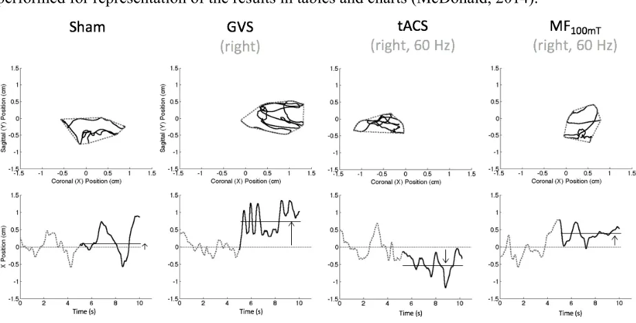
Figure 8: A representation of sway path (top panels dotted line), area (top panels solid line), and displacement along the coronal axis (bottom panels) for a single participant in the sham (first left panels), GVS (second to the left panels), tACS (second to the right panels), and MF100mT (right

(9)

show a clear displacement of the COP on the right during the GVS stimulation and a tendency to move on the left during the tACS stimulation. The MF100mT exposure seem to be associated with a

small displacement of the COP on the right (although not confirmed by statistical tests), and the sway stays unchanged during the sham condition as expected. ... 40

Figure 9: A representation of Coronal Velocity (top panels) showing the 5 second pre-exposure period (dotted line) and 5-second exposure period (solid line). The Frequency Domain analysis on Coronal Velocity (bottom panels) is shown for a single participant with the dotted line separating the different bands. Both characteristics are shown for the sham (left panels), GVS (second from the left panels), tACS (second from the right panels), and MF100mT (right panels)

conditions in the case of right side exposure. The graphs shown are based on a single participant for visualization purposes of the selected sway characteristics. The visual inspection of these graphs show a clear increased Coronal Velocity during the GVS stimulation, and a high Power associated with the medium frequency band. There is a less clear velocity increase during the tACS stimulation, and a high power associated with the medium frequency band. The MF100mT

exposure seem to be associated with no change in Coronal Velocity, with a high power associated with the low and medium frequency bands. The sway stays unchanged during the sham condition as expected, with a high power associated with the low frequency band. ... 41

Figure 10: Effect of Exposure for the Path Length of (y-axis) variable representing all

participants in the tACS, MF50mT, and MF100mT conditions (x-axis). As shown, the tACS condition

had a higher path length (4.52 ±0.23) than the MF conditions (3.94 ±0.22 for MF50mT and 3.95

±0.25 for MF100mT), signifying a destabilization for tACS exposure compared to MF exposure. 43

Figure 11: The frequency domain analysis exploring the Frequency effect for Coronal Velocity (High Frequency Band), comparing tACS, MF50mT, and MF100mT conditions. The exposure effect

is shown in the left panel and the Exposure-Frequency interaction in the right panel. The left panel shows a lower percentage of the normalized power spectrum associated with tACS (0.16

±0.01) compared to the MF conditions (0.18 ±0.01 MF50mT, 0.19 ±0.01 MF100mT) in the HFB.

(10)

Figure 12: Effect of Side with the Lateral Coronal Displacement variable, representing all participants in each of the exposure conditions. The x-axis represents the type of exposure and the y-axis represents the lateral coronal displacement, with a negative value representing a left displacement and a positive value representing a right displacement. Light grey bars represent a right side exposure, while dark grey bars represent a left side exposure. This graph shows the side effect being attributed to the GVS exposure, with a left side exposure showing a left coronal displacement (-0.57cm ±0.14) and a right side exposure showing a right coronal displacement (0.70cm ±0.16). This is in line with effects expected from the positive control condition. ... 45

Figure 13: Path Length (average of combined frequency conditions and exposure side for all participants) in each of the exposure conditions. The GVS condition is significantly different than any other condition, showing a higher Path Length (11.57cm ±2.30) than Sham (3.86cm ±0.31), tACS (4.52am ±0.23), MF50mT (3.94cm ±0.22), and MF100mT (3.95cm ±0.25). The tACS

condition also shows a significantly higher path length than the MF conditions. A higher Path Length signifies a higher destabilization. ... 47

Figure 14: Graphs of selected sway characteristics revealing a significant stabilization effect with the MF exposure device on the head as compared to without in terms of Path Length (helmet on: 6.28cm ±2.54, helmet off 12.10cm ±4.25), Area (helmet on: 0.65cm2_{±0.40, helmet off: 2.69cm}2

(11)

List of Appendices

Appendix A: Health Science Research Ethics Board Approval. ... 63

Appendix B: All participant characteristics (n=22) taking part in the postural control study. ... 66

Appendix C: LabView Data Collection Program. ... 67

Appendix D: MatLab Program with Sway Calculations. ... 70

Appendix E: Letter of Information and Consent Form. ... 72

Appendix F: Advertisement for Study Participation. ... 78

(12)

List of Abbreviations

AC Alternating Current

COP Centre of Pressure

DC Direct Current

E-field(s) Electric field(s)

ELF Extremely low frequency

EMG Electromyography

GVS Galvanic Vestibular Stimulation

ICNIRP International Commission on Non Ionizing Radiation Protection

IEEE Institute of Electrical and

Electronics Engineers

KC Kinocilium

MF(s) Magnetic Field(s)

MRI Magnetic Resonance Imaging

SCM Sternocleidomastoid

SVV Subjective Visual Vertical

tDCS Transcranial Direct Current

Stimulation

tACS Transcranial Alternating Current Stimulation

VOR Vestibulo-Occular Reflex

VSR Vestibulospinal Reflex

(13)

Chapter 1 1 General introduction

Even though we cannot see them, magnetic fields (MFs) are a part of our everyday lives. Humans are exposed to both natural and manmade MF sources on a daily basis. In the following sections, we will explore sources of MFs in our daily environment and possible interactions of these fields with human body. More specifically, it has been reported that the vestibular system is particularly sensitive to MF exposures, including both static and time-varying MFs (Glover, Cavin, Qian, Bowtell, & Gowland, 2007; L. E. van Nierop, Slottje, Kingma, & Kromhout, 2013). Therefore, we are interested in exploring the functional consequences of a time-varying MF on the vestibular system through the investigation of one of its main outcomes: postural control. An overview of the vestibular system’s anatomy, physiology and main functions will be given, along with vestibular dysfunctions and commonly used methods for evaluating vestibular system functioning. Then, we will review the literature on the effects of static and time-varying MF exposures, the second of which has the property to induce electric fields (E-fields) and currents in biological structures. Next, the literature on the effects of electric current stimulation applied to the human vestibular system will be reviewed, followed by an overview of the possible mechanisms of action involved.

1.1 Magnetic fields and possible human body interactions

MFs can be produced by a magnet or by moving electric charges. These fields can either be static, such as those produced by a direct current (DC) source, or time-varying, produced by an alternating current (AC) source. A static MF will have a constant value over time, whereas a time-varying MF will have a changing value over time. Time-varying MFs are sub-classified into extremely low frequency (ELF, <300 Hz), low to medium frequency (300 Hz – 3 MHz), and high frequency (3 MHz – 300 GHz) MFs. For the purpose of this research, we will be focusing specifically on ELF MFs, such as those produced by power-lines (i.e. 50 and 60 Hz).

(14)

-6_{). MF values are proportional to current intensity (I) and the distance (r) from the source by the}

following equation: B = (µ*I)/(2*π*r). Therefore, MF values decrease quickly with increased distance from the source. This equation is used to calculate the flux density at a given distance r from the source (from an electric wire). For example, it can be used to calculate the flux density level produced by a power-line when standing 4 meters below it.

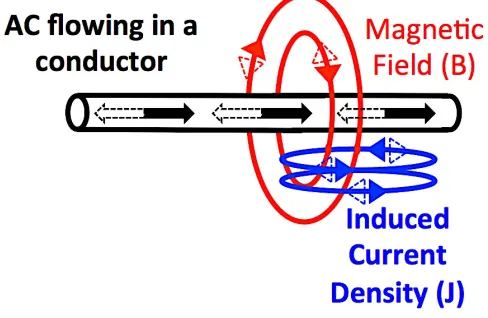
Time-varying MFs have the ability to induce electric fields (E-fields) and currents (expressed in terms of current density noted J). E-fields and induced current density are related by the following equation: E=J/s. The s value refers to conductivity, which is the capability of a material to conduct electricity; it is expressed in Siemens per meter (S/m). Figure 1 shows a visual representation of induced fields and currents created by a time-varying MF resulting from an AC source, such as a power line. Induced current density values are related to the conductivity of the material (s), the distance from the MF source (r), the MF value (B), and the MF frequency (f) as shown by the following equation (example of an AC current circulating in a wire): J = s*p*r*f*B. This formula can be used to calculate induced current density in a sphere of radius r of conductivity s by a time-varying MF of a given flux density (B) at frequency f.

Figure 1: MF-induced current density produced by an AC.

(15)

possibly causing a depolarization or hyperpolarization of the cell and therefore modulating transmitted neuronal signal. These potential interactions are discussed further in section 1.9.

1.2 Magnetic field sources in our daily environment

The main natural MF source is the Earth’s geomagnetic field. Manmade MFs result from electricity generation and distribution among other industrial processes. The Earth’s naturally produced geomagnetic field is mostly static (and cannot therefore elicit induced fields and currents in conductors or biological systems), reaching values at Earth’s surface of 35-70 µT (0.035-0.07 mT) according to the World Health Organization (WHO, 2006). Manmade MFs can be static, such as MRIs (up to 11 T or 11,000 mT) or time-varying, such as those produced by power-lines.

Average residential power-frequency MFs are 0.07 µT in Europe (50 Hz) and 0.11 µT in North America (60 Hz) (WHO, 2007). When considering average exposure levels for the general public including both residential and rural areas, the value is 0.1 µT at power-line frequencies according to the International Commission on Non-Ionizing Radiation Protection (ICNIRP, 2010). Additional information presented by the New Zealand Ministry of Health (2013) showed that MF values inside a house or office reached 0.05 – 0.15 µT. These values can rise when near a switchboard (1.0 – 3.0 µT, measured at a 300 mm distance from the source) or when standing directly under power lines, reaching values of 20 µT for 225 kV power lines and 30 µT for 400 kV power lines (Lambrozo, 2013).

Considering electrical household appliances, mean MF exposure levels are highest among microwave ovens (> 0.6 µT, at 2.45 GHz), coffee grinders (> 0.6 µT), electric shavers (0.3 µT), and electric hair dryers (0.3 µT) (Mezei et al., 2001). These MF values are based on measurements using a portable device. Higher MF values can be found when measurements are taken closer to the MF source. For example, when measuring at a distance of 3 cm from the source, exposure levels can reach up to 2 mT when using hair dryers (Gauger, 1985), electric hair clippers (Gandhi et al., 2001), electric shavers and electric drills (Lambrozo, 2013).

(16)

higher than average exposure levels for the general public. Gandhi et al. (2001) have identified exposure levels of above 1 mT for power line operators and for those working closely with high current conductors, such as live-line electric utility workers, exposure levels can reach up to 10 mT (WHO, 2007). With many humans being exposed to ELF MF sources in their everyday lives, it is important to consider potential interactions MFs could have on our biology and behavior.

1.3 Best known acute effect of MF on humans

With workers and citizens being exposed to MFs daily, several organizations, such as the WHO, the Institute of Electrical and Electronics Engineers (IEEE), and the ICNIRP, are working at providing comprehensive reviews of the literature and establishing health and safety guidelines for human MF exposure (Gowland & Glover, 2014; ICNIRP, 1998; IEEE, 2002; WHO, 2007). The WHO continues to encourage research on the health effects of MFs on humans through its international EMF project, initiated in 1996, as data is still needed to further establish safe international exposure. In order to inform the safety exposure guidelines, these organizations use evidence from the most well-established acute biological effect of induced electric fields in human tissue to date: magnetophosphene perception (ICNIRP, 2010).

(17)

depolarization, on the order of 0.6 to 200 µV (Attwell, 2003), they could be the most responsive targets for such exposures.

Interestingly, retinal rod cells share many physiological and functional similarities with vestibular hair cells as both cells use graded potentials for signal processing (Juusola, French, Uusitalo, & Weckstrom, 1996). Graded potentials indicate continuous variations in resting membrane potentials, as opposed to the characteristic all-or-none action potential. Vestibular hair cells are the functional units of the human vestibular system, which is responsible for maintaining balance. Due to the aforementioned similarity between retinal rod cells and vestibular hair cells, there is the possibility that vestibular system functioning could also be affected by power-line frequency MFs.

1.4 Vestibular anatomy, physiology, and function

1.4.1 Vestibular anatomy

The vestibular system, responsible for gaze control and maintaining balance, is located in the inner ear (one on each side of the head). It is located approximately 2.5 cm from the beginning of the external auditory canal and is approximately 2 cm long, about the size of a dime (James Byron Snow, 2009; Tortora & Nielsen, 2012). Its main structure consists of a series of membranous tubules filled with endolymph fluid (the labyrinth), which is continuous with the auditory component of the inner ear, known as the cochlea.

There are two main components of the vestibular system: the semicircular canals and the otolith organs. Each of the three semicircular canals are perpendicular to each other and are responsible for detecting a specific angular acceleration corresponding to pitch, yaw, and roll movements of the head. The otolith organs, the utricle and saccule, are responsible for detecting horizontal and vertical linear acceleration of the head, respectively. A localized dilation, known as the ampulla, is situated at the end of each semicircular canal duct.

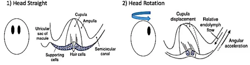
1.4.2 Vestibular physiology

(18)

cupula) to bend and either depolarize or hyperpolarize depending on the direction of fluid movement and hair cell orientation. Hair cells in the semicircular canal are oriented so that the tallest cilium, known as the Kinocilium (KC), is closest to the ampulla (Figure 2). This causes

increased or decreased firing rates of the afferent nerves on which the hair cells synapse. The otolith organs behave in a similar fashion. The difference is the use of shifting otoconia (calcium carbonate crystals) located in the otolith membrane to stimulate the hair cells and detect movements instead of endolymph fluid movement (Figure 3). The hair cells in the otolith organs are oriented relative to the striola, with the KC closest to the striola.

Figure 2: Hair cell movement detection in the semicircular canals. Figure adapted by author from Baloh et al. (2011). The adaptation of this graphic is by permission of the copyright holder: Oxford University Press ©.

Figure 3: Hair cell movement detection in the otolith organs. Figure adapted by author from Baloh et al. (2011). The adaptation of this graphic is by permission of the copyright

holder: Oxford University Press ©.

(19)

afferent nerve: type 1 onto irregular afferents and type 2 onto regular afferents, both of which carry signals to the vestibular nuclei. The details of each specific type of cell are still unclear apart from their differences in shape and number of synapses. However, it is known that regular afferent nerves make up 75% of vestibular afferents (Baird, Desmadryl, Fernandez, & Goldberg, 1988; Goldberg, 2000; Highstein, Goldberg, Moschovakis, & Fernandez, 1987).

Figure 4: Vestibular hair cells and subsequent changes in firing rate when depolarized or hyperpolarized. Figure adapted by author from Baloh et al. (2011). The adaptation of this

graphic is by permission of the copyright holder: Oxford University Press ©.

1.4.3 Vestibular function

The vestibular system is responsible for two main functions organized around two reflex loops: the vestibulo-ocular reflex (VOR) and the vestibulo-spinal reflex (VSR). Both reflexes together, in combination with visual, proprioceptive, and auditory information, globally control overall postural stability.

The VOR acts to stimulate certain muscles that control eye movements in response to head movements in order to stabilize images in our surrounding. This involuntary reflex allows us to perceive the world around us clearly even if we are moving. The VOR uses the semicircular canals and the otolith organs to detect and correct for head accelerations.

(20)

transmitted via the vestibule-spinal tracts to the spinal cord. Activation or inhibition of appropriate muscles will ultimately stabilize the body in response to a head tilt movement.

1.5 Vestibular diagnostic tests and disorders

There are many diagnostic tests used to stimulate the vestibular system and thereby test its functioning. Many physicians can achieve a better understanding of vestibular functioning by analyzing the two main reflex loops previously mentioned: VOR and VSR (Lang & McConn Walsh, 2010). Each of these loops can be assessed by first stimulating the vestibular system using different clinical tests and then analyzing selected variables to assess vestibular performance. We will cover the common variables assessed in each of the main clinical tests in this section, followed by a brief explanation of common vestibular disorders.

The first relatively simple diagnostic test is known as the Halmagyi test, which involves instructing the patient to fixate their eyes on a target directly in front of them while rapidly turning their head from side to side (in a yaw movement). This triggers the VOR for assessment. An individual with a compromised vestibular system would have difficulty fixating their gaze while rapidly moving their head. Similarly, the Rotary Chair test can also be used to assess the VOR, using a rotating chair instead of self-directed head movements to trigger the VOR. The VOR should be tested at low frequencies (0.5-5 Hz) using an active, voluntary, freely moving head rather than a rotating chair test in order to simulate natural activities (Dieterich & Brandt, 1995).

Another test exploring the VOR is known as the caloric reflex test. This test involves irrigation of warm or cool liquid through the external auditory canal and can specifically test for functioning of the nearby horizontal semicircular canal. The resulting temperature change in the external auditory canal induces convection currents in the nearby horizontal semicircular canal, which should induce an artificial perception of yaw rotational acceleration. Absence of resulting eye movement compensations due to VOR indicates weakness of the horizontal semicircular canal on the side of the head that is being irrigated (Goncalves, Felipe, & Lima, 2008).

(21)

ipsilateral to the side of the head experiencing the auditory clicks (Bath, Harris, & Yardley, 1998). VEMP testing is a useful diagnostic test for peripheral and central vestibulophathies (Roceanu, Schoenen, De Pasqua, & Bajenaru, 2010). A study by Welgampola and Colebatch (2005) found that assessing the VEMP in response to auditory clicks is the current best fit for the role of an otolith function screening test. Similarly, the head drop test can test for VSR functioning. This test is performed by having a patient lie down with their head suspended about 10 cm above a cushioned surface and allowing it to drop down. Responses of the neck muscles to this motion will determine the functionality of the VSR (Ito et al., 1995).

All of the previously mentioned diagnostic tests aim to stimulate the vestibular system in some way. We will now cover the variables that are analyzed during these tests. First, the variable assessed for VOR testing is nystagmus, a rapid vertical or horizontal eye movement. This can be recorded using electronystagmography, which uses electrodes placed around the eye to record eye movements or videonystagmography, which uses an infrared camera to track eye movements. In terms of the VSR testing, the variable recorded here is electromyographic (EMG) activity in the neck muscles, specifically the sternocleidomastoid muscle. Another variable that can be tested is known as the Subjective Visual Vertical (SVV). This is a measure of what patients perceive to be a true vertical compared to actual vertical. SVV can be used to specifically analyze the functioning of the utricle (Lang & McConn Walsh, 2010). Finally, posturography describes the recording of patient standing balance patterns (postural control) using a force platform. The force platform will measure center of pressure (COP) movements, which can be further analyzed for an overall stability assessment.

(22)

1.6 The vestibular system and electric stimulation

The previous section explored manipulation of the human vestibular system for the purpose of diagnostic testing and different variables that can be used to assess vestibular functioning. Interestingly, there is a specific type of electric stimulation using a direct current (DC) that targets the vestibular system, known as galvanic vestibular stimulation (GVS). GVS has been used in diagnostic testing and is known to reliably produce a loss of balance in humans. GVS therefore serves as a useful comparison point when studying the effects of MFs on postural control and so we will explore it further in the following section.

1.6.1 Transcranial Direct Current Stimulation (tDCS) – Galvanic

Vestibular Stimulation (GVS)

tDCS consists of delivering an electrical signal to the head using 2 or more skin electrodes (an anode and a cathode). When this technique is applied to the vestibular system, it is called galvanic stimulation. More specifically, galvanic stimulation consists of a non-invasive DC stimulation of the vestibular system (GVS) with electric currents on the order of 1 to 2 mA. This can result in spectacular changes in postural control and balance. The typical observed effect of GVS exposure in healthy participants is a body tilt towards one side occurring 1-2 seconds after the onset of the stimulation (Inglis, Shupert, Hlavacka, & Horak, 1995). Measurement of the displacement of the COP using a tracked marker placed on the head while exposed to GVS reveals an increase of the total length of the displacement of the COP over a given period of time (called path length) (Day, Severac Cauquil, Bartolomei, Pastor, & Lyon, 1997). A study using sway recordings from a force pate over a period of 5 s revealed peak COP displacements up to 4.5 cm laterally from the center of pressure (Yang et al., 2015). They also found a threshold of GVS exposure producing an acute postural control response to be 0.32 mA.

(23)

regardless of the hair cell orientation. This is different to natural movements, which would typically affect the hair cell orientation and then translate that signal onto the afferent nerves. Interestingly, regular afferent neurons are only minimally affected by GVS and it is the irregular afferent neurons that are largely affected. This signal from the vestibular afferents of the semicircular canals signals a large roll and small yaw movement directed away from the stimulation anode electrode. The signal from the vestibular afferents of the otoliths signals a linear acceleration away from the anode. The typical observed tilt response directed towards the anode is due to the VSR compensating for these perceived movements.

Now that we have overviewed the suspected mechanism of action behind the GVS response being due to induced currents, it is important to consider what levels of current exposure are reaching the human vestibular system with different GVS current levels. Nadeem et al. (2003) predicted that a 100 mA/m2 current density can be induced in brain tissue near the inner ear (3 cm deep from the external part of the head model) with a 1 mA current. Miranda et al. (2006) modeled the current distribution of tDCS using a 2.0 mA exposure. It was concluded that maximum values of 100 mA/m2, corresponding to a 0.22 V/m electric field, could be obtained at levels 3.5 cm below the scalp. Salvador et al. (2012) studied the effects of tissue dielectric properties on the electric field produced by tDCS using a head model. This study highlighted the importance of taking appropriate conductivities of different regions in the head when calculating the induced electric fields produced by tDCS. This highlights the complexities of predicting the exact induced electric fields produced in the human head using modeling studies. In terms of the level of the vestibular system, numerous different fluids and structures with different conductivities must be considered, complicating the induced electric field prediction process.

1.6.2 Transcranial alternating current stimulation (tACS)

(24)

possibility of the tACS stimulation interrupting the ongoing oscillations in the brain. This possibly achieved by inducing synchronizing changes in brain activity, modulating synaptic vesicle release, or by changing the level of electrical noise (Zaghi et al., 2010).

A rat study (Jensen & Durand, 2007) showed that applying high frequency (50-200 Hz) sinusoidal waves using AC stimulation could disrupt cell axon communication activity and this effect is dependent on the amplitude and frequency of the stimulus, not the stimulus duration. Kanai et al. (2010) explored cortical excitability by delivering tACS to the human occipital cortical region of the brain (at frequencies of 5, 10, 20, and 40 Hz) and reported the perception of phosphenes, a flickering visual phenomenon explained previously in section 1.3. They found that the 20 Hz frequency condition increased visual cortex excitability as indicated by the reported phosphene threshold. They proposed that tACS modulation of cortical excitability is frequency-dependent and that phosphenes are created due to tACS interaction with the visual cortex, not the retina. This is interesting since magnetophosphenes produced by time-varying MFs are thought to be due to induced electric fields with retinal rod cells, suggesting that the mechanism of action for tACS and MF exposure differs (Attwell, 2003). However, this hypothesis has been proven wrong in a study confirming that the effects observed by Kanai were actually resulting from a retinal stimulation (Laakso & Hirata, 2012).

To study tACS exposure effects on the human vestibular system, it is important to consider the current density distribution in the brain through a review of modeling studies. When considering the current density values reaching the thalamus (the deepest portion of the brain), a maximum current density of 50 mA/m2 can be reached using a 1 mA stimulus applied to electrodes placed behind the ear (Ferdjallah, Bostick, & Barr, 1996). This corresponds to an electric field value of 0.15 V/m. Induced electric fields reach maximal values (0.198 V/m using a 1.12 mA tACS exposure) just beneath the electrode surface (Merlet et al., 2013). No modeling studies have been found regarding tACS induced current and electric field values at the level of the vestibular system.

(25)

combine static MF and time-varying MFs (Glover et al., 2007; L. E. van Nierop et al., 2013; L. E. van Nierop, Slottje, van Zandvoort, de Vocht, & Kromhout, 2012). The following selected studies are presented in order of the variable studied. We will first present studies of postural control responses followed by studies of nystagmus.

Theysohn et al. (2014) studied vestibular effects of a 7 T MRI (7,000 mT for comparison) compared to 1,500 mT and 0 mT in healthy volunteers. 46 healthy participants were recruited and exposed for 30 minutes to static MFs. Postural control recordings using a force plate were taken at 3 different time intervals (before exposure, 2 minutes after and 15 minutes after exposure). Their results showed a significant increase in the average size of oscillations (quantified using mean sway path and sway path length characteristics) at the 2-minute post-exposure mark (compared to the pre-post-exposure period). This normalized back to pre-post-exposure values at the 15-minute post-exposure mark. They surmised that these changes are attributed to the vestibular system since proprioceptive feedback was minimized during the experiment and conditions with the eyes opened showed suppressed effects.

Glover et al. (2007) investigated several aspects of static MF exposure and how they affected vestibular system functioning, using a 7 T MRI. They studied vertigo with respect to static, pulsed, and time-varying MF. The latter two results will be discussed in the following sections. For the static MF condition, participants were asked to stand either close to (B = 800 mT) or further from (B = 200 mT) the MRI while sway movements were tracked using a video camera. In 3 of 10 participants a significant mean forward displacement was found in the near position compared to the far position. Two of the subjects perceived a falling sensation in the near position, a description consistent with vertigo as commonly described in clinical settings. It should be noted that the experience of vertigo is linked to the vestibular system since vertigo is described as a perception of motion in the absence of actual mechanical motion and perception of motion occurs at the level of the vestibular system. Vertigo could also arise from an inconsistency between visual input and actual mechanical motion. Similarly, there is a clear vestibular pathway for nausea and vomiting (Horn, 2008). Some studies have used the basis of this pathway as an outcome to measure vestibular functioning in MRI studies. Such studies will be presented in the following section.

(26)

infrared video recording from when the participant entered the MRI bore to when they exited. Ten participants with normal labyrinthine function were tested along with two participants with no labyrinthine function. Normal labyrinthine function is defined as having an intact and functional labyrinth. It was confirmed that labyrinthine function was necessary to induce nystagmus as healthy subjects developed a robust nystagmus while in the MRI and participants with no labyrinthine function did not. For healthy participants, the magnitude of the induced nystagmus was dependent on the strength of the time-varying MF (induced by movement through the static MF), implying that stronger time-varying MFs that are induced by movement through the static MFs have a stronger effect on the vestibular system, particularly the VOR.

Mian et al. (2013) exposed 25 participants to a static MF produced by a 7 T MRI while recording eye movement patterns and reported sensations of motion. All participants had clear nystagmus while being pushed into the MRI. Values peaked shortly after arriving in the MRI and slightly declined over time spent in the MRI. This is interesting since movement within a static MF is considered a time-varying MF. Therefore, as the participants are being moved into the MRI while the static MF is present with a gradient, they are being exposed to a time-varying MF. Additionally, 24 of the 25 participants reported perceptions of motion (or vertigo). They also discovered that the onset of the perception of motion (~5.1 T) occurred at a significantly higher field strength than nystagmus onset (~1.7 T). The results of this study involving static MF evoked perception of motion is in line with the MF evoked nystagmus observed by the normal patient group of the Roberts et al. (2011) study.

(27)

1.8 The vestibular system and time-varying magnetic fields

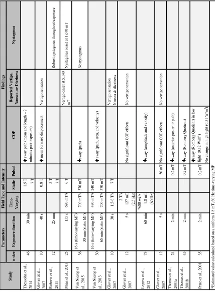
The impact of research on the effects of ELF MFs on the human vestibular system has been limited to date due to the difficulty in reproducing experimental results and the diversity of exposure protocols used. This makes it difficult to compare the results from different studies (see Table 1 for summary). The results of these studies will be discussed below.

Van Nierop et al. (2013) used a combination of static and time-varying MF exposure using an MRI to assess MF effects on postural control. Time-varying MFs were produced using standardized head movements while participants stood next to a 7 T MRI. Participants stood on a force plate to assess their postural control immediately after inducing the time-varying MF via head movements. Subjects were exposed to a sham, low (490 mT/s), and high (700 mT/s) time-varying MF for 16 seconds, during which they performed 10 vertical and 10 horizontal head movements on 3 separate occasions. The static MF was present the entire time during the high and low exposure conditions (low = 240 mT and high = 370 mT), but was not present during the sham condition. Results showed an increase in the size and the velocity of the sway pattern (as measured using sway path, area, and velocity characteristics) upon exposure to the induced varying MF compared to sham. Higher exposure levels had a greater effect. Since the time-varying MFs were induced with head movements within a static MF, participants were exposed to both types of MFs. Therefore, it is not possible to distinguish whether the observed effects were due to the time-varying MF or static MF component.

(28)

Results showed a significant interaction between static MF + time-varying MF exposure and unilateral weakness in all tasks. This included a stabilization effect (decreased sway path) in the static MF+time-varying MF condition compared to the sham condition for those with unilateral horizontal canal weakness. In terms of the cognitive function tasks, the static+time-varying MF condition showed significantly decreased verbal memory and visual acuity compared to sham.

(29)

Table 1: Summary of studies exploring the effects of MFs on human standing balance. n -s iz e Exp os u re d u rati on Ti me -V ar yi n g S tati c Pulsed COP R ep or te d V er ti go, N au se a, or D iz zi n es s N ys tagmu s

1.5 T 7 T

G love r a t a l., 2007 10 40 s 0.8 T é m ea n forw ard di spl ac em ent V ert igo s ens at ion

3 T 7 T

M ia n e t a l., 2013 25 135 s 690 m T /s 6 T V ert igo ons et a t 5,140 mT N ys ta gm us ons et a

t 1,670 m

T 16 s (t im e-va ryi ng M F ) 30 m in (s ta ti c M F ) 16 s (t im e-va ryi ng M F ) 490 m T /s 240 m T 65 m in (s ta ti c M F ) 700 m T /s 370 m T G love r e t a l., 2007 10 30 s 1.5-6 T /s 7 T V ert igo s ens at ion N aus ea & di zz ine ss 2 T /s 127 m T (2.5 H z) *680 m T /s 1.8 m T (60 H z) G love r e t a l., 2007 12 5 s 50 m T N o s igni fi ca nt CO P e ffe ct s N o ve rt igo s ens at ion T hom as e t a l., 2001a 24 2 m in 0.2 m T ê sw ay (a nt eri or-pos te ri or pa th) T hom as e t a l., 2001b 45 2 m in 0.2 m T ê sw ay (Rom be rg Q uot ie nt ) é sw ay (Rom be rg Q uot ie nt ) i n l ow li ght ( 0.12 W /m 2) N o c ha nge in hi gh l ight (0.51 W /m 2 ) 60 m in *E st im at ed va lue c al cul at ed ba se

d on a

uni

form

1.8 m

T

, 60 H

z t im e-va ryi ng M F 0.2 m T 2 m in 35 P ra to e t a l., 2001 V an N ie rop e t al ., 2013 73 L egros e t a l., 2012 N o ve rt igo s ens at ion N o s igni fi ca nt CO P e ffe ct s 5 s 12 G love r e t a l., 2007 ê sw ay (a m pl it ude a nd ve loc it y) é s w ay (pa th, a re a, a nd ve loc it y) 30 36 V an N ie rop e t al ., 2015 Robus t nys ta gm us throughout e xpos ure 25 m in 12 Robe rt s e t a l., 2011 N o nys ta gm us ê sw ay (pa th) 370 m T 700 m T /s 46 T he ys ohn e t a l., 2014 F in d in gs F ie ld Typ e an d I n te n si ty P ar ame te rs S tu d y é s w ay pa th (m ea n a nd l engt

h – 2

(30)

Glover at al. (2007) also studied the effects of time-varying MFs on the vestibular system by assessing postural control using force plate data. This study combined three protocols in which participants were exposed to different MF exposures: a static MF (static subject), a static MF (moving subject), and a time-varying MF (static subject). The first protocol was described in the previous section as significantly increasing mean forward displacement. The second protocol involved moving the participants slowly into the static MF of the 7 T MRI and then instructing them to make uniform head movements once positioned there. For this condition, participants were lying down in the MRI and they described their overall experiences. Results from this condition showed that 7 of 10 participants reported perceived movement inconsistent with their actual movement in the moving participant condition. MF-induced vertigo effects (9 of 10 participants) such as nausea (2 of 10 withdrew due to severe nausea) and dizziness (8 of 10) were also reported. The third protocol involved a time-varying MF with a static subject. Subjects were exposed to a MF at 5-second intervals during eight 1-minute trials while standing on a force plate for COP assessment. Four exposures used a sinusoidal stimulus (2.5 Hz, 2,000 mT/s, 127 mT peak) and four used a pulsed stimulus (0.5 s duration, 2,000 mT/s, 50 mT peak). Results showed that there was no detected effect of MFs on COP and there was no reported sensation of sway by the subjects. This study is significant in that it delivered a time-varying MF independent of a static MF through a solenoid coil exposure system. Unfortunately, the result of the static MF (moving subject) condition is not directly comparable to the other two protocols since COP could not be analyzed with the subjects lying down. However, it seems as though there is a destabilization effect in response to static MF exposure and no exposure effect for time-varying MF or pulsed MF exposures. This suggests that perhaps movement-induced time-varying MF exposures within an MRI are due to the constant presence of the static MF. It could also suggest that the time-varying MF produced with these head movements is significantly different from those produced by solenoid coils. The fact that different outcomes that may not result from the same neurophysiological pathways are reported makes interpretations difficult.

(31)

higher frequency, which brings the dB/dt in the same order of magnitude (680 mT/s in the Legros’ study). Participants were exposed for 1 hour after which they completed a series of tasks, including a postural oscillation recording. Force plate recordings showed a stabilization effect in terms of decreased velocity and amplitude of postural control oscillations for the MF condition compared to the sham condition. These effects were only observed during the eyes closed conditions. This suggests that the time-varying MF acts on proprioceptive or vestibular functions, a finding consistent with results from Glover et al. (2007). Comparing COP of Glover at al. (2007) and Legros et al. (2012), there appears to be some discrepancies in that no stabilization or destabilization effects were found for the former and a significant stabilization effect was found for the latter. This could be due to significant differences in the exposure apparatus between the two studies, thereby changing the MF distribution patterns. For example, Glover at al. (2007) used a 2.5 Hz stimulus, compared to a 60 Hz stimulus used by Legros et al. (2012). Therefore, it is possible that a frequency threshold somewhere between 2.5 and 60 Hz determines the observed stabilization response. A single study testing different frequency levels at a single MF value could provide more information on potential threshold effects. Indeed, considering the previous studies, there is likely a threshold effect to be determined in terms of exposure time, frequency, and intensity. The study we are conducting will address this possibility, as explained in the following chapters. Another consideration possibly accounting for observed differences in postural control results is the stance of each participant on the force plate. Van Nierop et al. (L. van Nierop, 2015; L. E. van Nierop et al., 2013) had participants stand with their feet together in a parallel position (0 cm apart) on a foam layer, whereas Legros et al. (2012) had participants stand with 1 cm between the feet in a parallel position with no foam layer. Glover et al. (2007) also used a foam layer, but provided no information on the spacing of participants’ feet. It is therefore possible that the destabilization effects noted in the van Nierop et al. (2013) study was found due to the participants being in a less stable position than the positioning reported by Legros et al (2012).

(32)

stabilization effect in terms of center of pressure. This was primarily observed through a decrease in distribution (range) of front–back motion. A second study (Thomas, White, et al., 2001) compared the effects of the same pulsed (0.2 mT, 700 mT/s, 0-500 Hz) MF between fibromyalgia, rheumatoid arthritis, and healthy individuals, using a similar experimental design as Thomas et al. (2001). Results again showed a significant stabilization effect in terms of an improved (decreased) Romberg Quotient (COP length in eyes closed measure divided by COP length in the eyes open measure (Nardone, Tarantola, Giordano, & Schieppati, 1997) upon exposure to the pulsed MF compared to sham. Levels of improvement differed between healthy patients and fibromyalgia or rheumatoid arthritis patients, suggesting an application in terms of diagnosis using pulsed MFs. Another experiment (Prato, Thomas, & Cook, 2001) studied the effects of a pulsed MF (0.2 mT, 700 mT/s, 0-500 Hz) on postural control in different low (0.12 W/m2) and high (0.51 W/m2) intensity light conditions. A force plate recorded COP patterns and the Romberg Quotient was used for analysis. The pulsed MF condition showed a significant destabilization effect (increased Romberg Quotient) compared to sham under the low light condition only. This suggests a light-dependent effect of pulsed MFs on human postural control with lower light levels having more of a destabilization effect compared to high light levels. Considering the previous three studies, it appears that this particular stimulus (0.2 mT, 700 mT/s, 0-500 Hz MF) can have a stabilizing effect except for in low light conditions where it has a destabilizing effect. This is coherent with the proposal that a destabilization of postural control leads to a greater effect of MFs on the vestibular system. This is achieved, for example by having participants close their eyes or reduce the lighting levels and having them stand with their feet directly together. No further studies have been found on the effects of pulsed MFs on human postural control.

(33)

using low light conditions, there can be a destabilization effect as well. Since very few studies have been conducted in this research area, it is difficult to make direct comparisons. Further research is warranted to be able to better explain some of these discrepancies. Additionally, these studies do not inform us about potential mechanisms of action for vestibular responses to time-varying MF exposure. We will attempt to explore this in the next section.

1.9 Proposed mechanisms of action for MF exposure

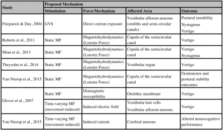
There are a number of studies that explore the mechanism of action behind the observed effect of vestibular disruption due to MFs (see Table 2 for summary). In this section, we will explore the plausibility of the three main proposed mechanisms of action, as proposed by Glover et al. (2007): Magnetohydrodynamics, diamagnetic susceptibility, and induced electric fields and currents. It is noted that mechanisms of action proposed for direct current sources (GVS) were previously explored separately in section 1.6.1. This is because mechanisms of action proposed for a direct current source are not easily comparable to proposed mechanisms of action from an alternating current or time-varying MF source.

Table 2: Summary of proposed mechanisms of action for MF exposure.

Stimulation Force/Mechanism Affected Area Outcome Postural instability Nystagmus Vertigo

Roberts et al., 2011 Static MF Magnetohydrodynamics (Lorentz Force)

Cupula of the semicircular

canal Vertigo

Vertigo Nystagmus

Theysohn et al., 2014 Static MF Magnetohydrodynamics

(Lorentz Force) Vestibular organ Vertigo

Van Nierop et al., 2015 Static MF Magnetohydrodynamics (Lorentz Force)

Cupula of the semicircular canal

Oculomotor and postural stability outcomes

Static MF Diamagnetic

susceptibility Otolithic membrane Vertigo Vestibular hair cells

Vestibular afferent neurons

Van Nierop et al., 2015 Time-varying MF

(movement-induced) Induced current Cerebral neurons

Altered neurocognitive performance

Vestibular afferent neurons (otoliths and semi-circular canals)

Direct current exposure GVS

Fitzparick & Day, 2004

Proposed Mechanism Study

Vertigo Induced electric field

Time-varying MF (movement-induced) Glover et al., 2007

Cupula of the semicircular canal

Magnetohydrodynamics (Lorentz Force) Static MF

(34)

1.9.1 Magnetohydrodynamics

The first proposed mechanism, magnetohydrodynamics, describes the flow of conducting fluids (such as blood or endolymph fluid) in electromagnetic fields and how these fields allow for forces to arise in the fluid due to induced currents. These forces act on the cupula and thereby cause a perceived accelerated movement. This is the widely accepted mechanism of action described for the observed effects of static MF exposure on vestibular functioning. We will present studies that explain this effect in terms of static MFs followed by the potential for magnetohydrodynamics to be applied to time-varying MFs.

A study by Roberts et al. (2011) proposed the Lorentz force (one of the forces described by magnetohydrodynamics) as the cause of vertigo sensation for participants in the static field of an MRI. This force was described as a resulting interaction between ionic currents in the endolymph fluid (within the labyrinth of the vestibular system) and the MF. Specifically, forces due to the interaction of the MF with the induced ionic current become noticeable when they have a similar magnitude to the inertial force of the fluid, potentially causing perceived movements. These forces act directly on the semicircular canal cupula (see section 1.4.2), which upon bending, leads to stimulation of the adjoining hair cells and therefore the hair cells themselves are not directly affected. The calculated pressure exerted by the Lorentz force on the cupula (0.002-0.02 Pa) by a 7 T MRI exceeds the nystagmus threshold (0.0001 Pa), thus being a sound proposal for the mechanism of action behind the observed nystagmus. Further modeling work by Antunes et al. (Antunes, Glover, Li, Mian, & Day, 2012) supported the hypothesis of a Lorentz force being a significant contributor to static MF-induced nystagmus as reported by Roberts et al. (2011) and Mian et al. (2013).

(35)

proposed mechanism, MF induced nystagmus and vertigo is therefore not dependent on movement inside MFs, MF gradients, or time-varying MFs. Rather, it is dependent on naturally occurring ionic currents in the endolymph fluid, which can be modulated by MF magnitude and direction.

Theysohn et al. (2014) used previous literature combined with their test results to determine the mechanisms of action for induced vertigo within the static MF of MRIs. They surmised that vertigo generation was not caused by the gradient system or the radiofrequency excitation, since turning off each of these components in turn did not diminish the observed postural instability effect. Overall, they proposed that a compensatory response in the vestibular organ, similar to the mechanism of action proposed by Roberts et al. (2011), explains the observed vertigo effects as they were only detected after a prolonged exposure in a static MF with no participant movement.

Glover at al. (2007) looked into the applicability of magnetohydrodynamics to time-varying MF effects on the vestibular system. They concluded that these magnetohydrodynamic forces are unlikely to be of relevance in the vestibular system due to the small size of the vestibular structure and the fluid conductivities being too low to induce such a force. However, they suggested it is possible to see these effects in larger arteries or at MFs greater than 7 T (Kangarlu & Robitaille, 2000). Van Nierop et al. (2015) support this in concluding that a 1,000 mT static MF induced Lorentz force would be too weak to produce a detectable horizontal nystagmus. Considering this, it seems that magnetohydrodynamics serve as an excellent basis for explaining the effects of static MFs on the vestibular system in MRIs, which have the ability to produce large MF values above 7 T. Alternatively, they cannot be applied to the studies conducted so far on time-varying MFs which use much lower magnetic flux densities. This difference in proposed mechanisms of action for static compared to time-varying MFs could also explain some of the discrepancies found in standing balance studies as discussed in the previous section (section 1.8).

1.9.2 Diamagnetic susceptibility

(36)

in density and therefore magnetic susceptibility between the otoliths and their surrounding fluid. Glover et al. (2007) support this mechanism of action to describe the observed sway modifications for subjects standing near the MRI as it is the only mechanism described that is not dependent on movement within the field. It is noteworthy to include that it is highly difficult to assess the effects of this mechanism on other structures of the vestibular system. Indeed, structures such as the semicircular canals have different fluid dynamics and densities to consider. No other studies have directly reported on this mechanism of action in terms of MF exposure in human.

Diamagnetic susceptibility has also been studied in the context of animal orientation and homing abilities. A homing ability is an animal’s ability to return to a given location after traveling a significant distance from it. It was found that in the presence of man-made electromagnetic noise, the homing mechanism of migrating birds was disrupted (Engels et al., 2014). A study by Wu and Dickman (2012) further explored the homing mechanism in pigeons in which they described special cells that code for MF intensity, direction, and polarity of earth’s geomagnetic field. These characteristics are all a necessary and integral part for animal homing abilities. With respect to humans, this mechanism may not be relevant in the vestibular system since humans do not possess the sensitivity in their vestibular cells to detect earth’s geomagnetic field of only 35-70 µT (Wu & Dickman, 2012).

1.9.3 Induced current and electric fields

(37)

in the vestibular system, causing a perceived motion. It is therefore possible that time-varying MFs of sufficient strength, which also have the capability of inducing a current, will have a similar effect at the level of the vestibular system.

Glover at al. (2007) proposed a similar mechanism of action, which they termed induced galvanic vestibular stimulation. This is described as changes in the electric field across the vestibular hair cells of the semicircular canal cupulae and otolithic membrane thus modulating their afferent neuron’s firing rate and giving an artificial perception of movement. They concluded that movements or rotations in gradients or homogeneous MFs could cause perceived movements via induced galvanic vestibular stimulation and that this is a polarity-sensitive effect. A polarity-sensitive effect is an effect dependent on a difference in charge for the anode compared to the cathode in terms of GVS. When considering the vestibular system this is seen as a difference in charge on one side of the head compared to the other. Versluis et al. (2013) also support induced current acting directly on hair cells as a viable mechanism of action.

(38)

References

Antunes, A., Glover, P. M., Li, Y., Mian, O. S., & Day, B. L. (2012). Magnetic field effects on the vestibular system: calculation of the pressure on the cupula due to ionic current-induced Lorentz force. Phys Med Biol, 57(14), 4477-4487. doi: 10.1088/0031-9155/57/14/4477

Attwell, D. (2003). Interaction of low frequency electric fields with the nervous system: the retina as a model system. Radiat Prot Dosimetry, 106(4), 341-348.

Baird, R. A., Desmadryl, G., Fernandez, C., & Goldberg, J. M. (1988). The vestibular nerve of the chinchilla. II. Relation between afferent response properties and peripheral innervation patterns in the semicircular canals. J Neurophysiol, 60(1), 182-203.

Baloh, R, Honrubia, V, & Kerber, K. (2011). Baloh and Honrubia's Clinical Neurophysiology of

the Vestibular System (4 ed.): Oxford University Press. Oxford, UK.

Bath, A. P., Harris, N., & Yardley, M. P. (1998). The vestibulo-collic reflex. Clin Otolaryngol

Allied Sci, 23(5), 462-466.

Bohnert, J., & Dossel, O. (2010). Effects of time varying currents and magnetic fields in the frequency range of 1 kHz to 1 MHz to the human body - a simulation study. Conf

Proc IEEE Eng Med Biol Soc, 2010, 6805-6808. doi: 10.1109/IEMBS.2010.5625970

d'Arsonval, A. (1896). Dispositifs pour la mesure des courants alternatifs de toutes fréquences. Société de Biologie, 450-451.

Day, B. L., Severac Cauquil, A., Bartolomei, L., Pastor, M. A., & Lyon, I. N. (1997). Human body-segment tilts induced by galvanic stimulation: a vestibularly driven balance protection mechanism. J Physiol, 500 ( Pt 3), 661-672.

Dieterich, M., & Brandt, T. (1995). Vestibulo-ocular reflex. Curr Opin Neurol, 8(1), 83-88.

Engels, S., Schneider, N., Lefeldt, N., Hein, C.M., Zapka, M., Michalik, A., Elbers, D., Kittel, A., Hore, P.J., & Mouristen, H. (2014). Anthropogenic electromagnetic noise disrupts magnetic compass orientation in a migratory bird. Nature, 509, 353–356. doi: 10.1038/nature13290

Ferdjallah, M., Bostick, F. X., Jr., & Barr, R. E. (1996). Potential and current density distributions of cranial electrotherapy stimulation (CES) in a four-concentric-spheres model. IEEE Trans Biomed Eng, 43(9), 939-943. doi: 10.1109/10.532128

(39)

Gandhi, O. P., Kang, G., Wu, D., & Lazzi, G. (2001). Currents induced in anatomic models of the human for uniform and nonuniform power frequency magnetic fields.

Bioelectromagnetics, 22(2), 112-121.

Gauger, J.R. (1985). Household appliance magnetic field survey. IEEE Transactions on Power

apparatus and systems, PAS-104(9), 2436-2444.

Glover, P. M., Cavin, I., Qian, W., Bowtell, R., & Gowland, P. A. (2007). Magnetic-field-induced vertigo: a theoretical and experimental investigation. Bioelectromagnetics, 28(5), 349-361.

Goldberg, J. M. (2000). Afferent diversity and the organization of central vestibular pathways. Exp Brain Res, 130(3), 277-297.

Goncalves, D. U., Felipe, L., & Lima, T. M. (2008). Interpretation and use of caloric testing.

Braz J Otorhinolaryngol, 74(3), 440-446.

Gowland, P., & Glover, P. (2014). Comment on ICNIRP guidelines for limiting exposure to electric fields induced by movement of the human body in a static magnetic field and by time-varying magnetic fields below 1 Hz. Health Phys, 107(3), 261. doi: 10.1097/HP.0000000000000142

Hain, T. C., & Helminski, J. O. (2007). Anatomy and Physiology of the Normal Vestibular System. In S. L. Wolf (Ed.), Vestibular Rehabilitation (3 ed.). Philadelphia: F.A. Davis Company. Phuladelphia, US.

Health, New Zealand Ministry of. (2013). Electric and magnetic fields and your health: Information on electric and magnetic fields associated with transmission lines, distribution lines and electrical equipment.

Highstein, S. M., Goldberg, J. M., Moschovakis, A. K., & Fernandez, C. (1987). Inputs from regularly and irregularly discharging vestibular nerve afferents to secondary neurons in the vestibular nuclei of the squirrel monkey. II. Correlation with output pathways of secondary neurons. J Neurophysiol, 58(4), 719-738.

Horn, C. C. (2008). Why is the neurobiology of nausea and vomiting so important? Appetite, 50(2-3), 430-434. doi: 10.1016/j.appet.2007.09.015

ICNIRP. (1998). Guidelines for limiting exposure to time-varying electric, magnetic, and electromagnetic fields (up to 300 GHz). International Commission on Non-Ionizing Radiation Protection. Health Phys, 74(4), 494-522.

(40)

IEEE. (2002). C95.6 - IEEE Standard for safety levels with respect to human exposure to electromagnetic fields, 0-3 kHz. IEEE: New York.

Inglis, J. T., Shupert, C. L., Hlavacka, F., & Horak, F. B. (1995). Effect of galvanic vestibular stimulation on human postural responses during support surface translations. J

Neurophysiol, 73(2), 896-901.

Ito, Y., Corna, S., von Brevern, M., Bronstein, A., Rothwell, J., & Gresty, M. (1995). Neck muscle responses to abrupt free fall of the head: comparison of normal with labyrinthine-defective human subjects. J Physiol, 489 ( Pt 3), 911-916.

James Byron Snow, Phillip A. Wackym. (2009). Ballenger's Otorhinolaryngology: Head and

Neck Surgery (17 ed.): People's Medical Publishing House. Shelton, USA.

Jensen, A. L., & Durand, D. M. (2007). Suppression of axonal conduction by sinusoidal stimulation in rat hippocampus in vitro. J Neural Eng, 4(2), 1-16. doi: 10.1088/1741-2560/4/2/001

Juusola, M., French, A. S., Uusitalo, R. O., & Weckstrom, M. (1996). Information processing by graded-potential transmission through tonically active synapses. Trends

Neurosci, 19(7), 292-297. doi: 10.1016/S0166-2236(96)10028-X

Kanai, R., Paulus, W., & Walsh, V. (2010). Transcranial alternating current stimulation (tACS) modulates cortical excitability as assessed by TMS-induced phosphene thresholds. Clin Neurophysiol, 121(9), 1551-1554. doi: 10.1016/j.clinph.2010.03.022

Kangarlu, A., & Robitaille, P.M.L. (2000). Biological effects and health implications in magnetic resonance imaging. Concepts Magn Reson, 12(5), 321-359.

Laakso, I., & Hirata, A. (2012). Computational analysis of thresholds for magnetophosphenes. Phys Med Biol, 57(19), 6147-6165. doi: 10.1088/0031-9155/57/19/6147

Lambrozo, J.; Souques, J. (2013). Electricity and Extremely Low Frequency Electric and Magnetic Fields. In S. S. B. Media (Ed.), Electromagnetic Fields, Environment and

Health.

Lang, E. E., & McConn Walsh, R. (2010). Vestibular function testing. Ir J Med Sci, 179(2), 173-178. doi: 10.1007/s11845-010-0465-7

Legros, A., Corbacio, M., Beuter, A., Modolo, J., Goulet, D., Prato, F. S., & Thomas, A. W. (2012). Neurophysiological and behavioral effects of a 60 Hz, 1,800 muT magnetic field in humans. Eur J Appl Physiol, 112(5), 1751-1762. doi: 10.1007/s00421-011-2130-x